Microproteomics: Quantitative Proteomic Profiling of Small Numbers of Laser-Captured Cells

INTRODUCTION

During the last decade, significant progress in the analysis of whole genomes and transcriptomes has triggered efforts to analyze the proteome. Advancements in protein extraction, purification, and identification have been driven by the development of mass spectrometers with greater sensitivity and resolution. Nevertheless, comparative and quantitative proteomic technologies have not progressed to the extent of genomic and transcriptomic technologies for accessing gene expression differences. Unlike the genome, which is similar throughout all cells in a given organism, the proteome varies in different cells. Also, there is no self-replicating amplification mechanism for proteins such as the polymerase chain reaction (PCR) for DNA. Therefore, developing methods that extract, separate, detect, and identify proteins from extremely small samples are needed. The advent of laser capture microdissection (LCM) has expanded the analytical capabilities of proteomics. LCM has proven an effective technique to harvest pure cell populations from tissue sections. This protocol describes a microproteomic platform that uses nanoscale liquid chromatography/tandem mass spectrometry (nano-LC-MS/MS) to simultaneously identify and quantify hundreds of proteins from LCMs of tissue sections from small tissue samples containing as few as 1000 cells. The LCM-dissected tissues are subjected to protein extraction, reduction, alkylation, and digestion, followed by injection into a nano-LC-MS/MS system for chromatographic separation and protein identification. The approach can be validated by secondary screening using immunological techniques such as immunohistochemistry or immunoblots.

RELATED INFORMATION

This protocol involves multiple stages, including tissue isolation by LCM, protein extraction and digestion, protein quantitation, protein identification, and biological verification (Fig. 1 ). In the following example, these techniques are used to screen for proteomic differences in two populations of brainstem motor nuclei from songbirds. These are (1) the 12^th motor nucleus, which controls the syrinx muscles (i.e., the avian vocal organ), and receives a direct projection from the forebrain only in species that can imitate vocalizations; and (2) the supraspinal (SSp) motor nucleus, which controls the neck muscles (in birds and mammals), and does not receive a direct forebrain projection and thus serves as control (Jarvis 2004).

FIGURE 1.

Flowchart for microproteomic screening protocol.

In this protocol, peptide sample digests are analyzed using nanoscale capillary LC/MS/MS. The type of analysis chosen will vary widely depending on the hardware and analytical tools available. The use of high-resolution, high-mass-accuracy mass spectrometers (e.g., quadropole/time-of-flight or Orbitrap instruments) is recommended; they allow for rigorous data collection and unbiased label-free quantitation via area-under-the-curve intensity measurements. Such systems produce highly sensitive analyses with low protein false-positive rates and accurate cross-sample quantitation (Carducci et al. 2001; Smith et al. 2002; Paša-Tolić et al. 2004; Silva et al. 2005; Tolmachev et al. 2008).

Individual peptides are quantified across all sample injections; integration of each chromatographic peak belonging to the same precursor mass in the aligned chromatograms is then used to calculate the peptide intensity in each LCM sample. Only data-independent mass spectrometry high energy (MS^E) data are used for quantitative measurements; data-dependent acquisition (DDA) data are also aligned and used to provide supplementary protein identifications but are not used for quantitation because of the low duty cycle in the MS dimension (only one data point per ~5 sec) (Silva et al. 2006; Geromanos et al. 2009; Li et al. 2009). Relative protein quantity within each sample is calculated as the sum of the intensity of each peptide to that protein. To detect changes in protein abundance with high precision, analyze each sample in triplicate, using two MS^E quantitative/qualitative runs and one qualitative DDA run.

MATERIALS

Reagents

• Acetonitrile (Sigma-Aldrich)

• Alcohol dehydrogenase digest (ADH1_YEAST; Waters)

• Ammonium bicarbonate (50 mM; Sigma-Aldrich)
• Animal of interest (for immunohistochemistry)

• Antibody, primary, specific to protein of interest

• Antibody, secondary, fluorescently labeled

• BCA (Bicinchoninic) assay kit, low-protein (Lamda Biotech)

• Dithiothreitol (DTT, 100 mM; Sigma-Aldrich)
• Embedding medium (e.g., Tissue-Tek OCT compound; Sakura Finetek)

• Ethanol (75%, 95% [both prepared with Invitogen ultrapure water], and 100%)

• Fluorescence mounting medium (e.g., VECTASHIELD; Vector Laboratories)

• Formic acid
• Iodoacetamide (200 mM; Sigma-Aldrich)
• Paraformaldehyde (4% in PBS) (Sigma-Aldrich)

• Phosphate-buffered saline (PBS; 1X)

• Serum, normal, species-specific

• Sucrose (30% in PBS)

• Tissue of interest

• Trifluoroacetic acid (TFA; Sigma-Aldrich)
• Trifluoroethanol (TFE; Sigma-Aldrich)
• Triton X-100
• Trypsin, mass spectrometry grade (e.g., Trypsin Gold; Promega)

• Water, distilled, ultrapure (Invitrogen)

• Xylene (Sigma-Aldrich)

Equipment

• Chromatography column, 1.7-μm C18 BEH, 75-μm x 250-mm (Waters)

• Chromatography column, Symmetry C18, 20-μm x 180-mm (Waters)

• Coverslips

• Cryomolds (Sakura Finetek)

• Cryostat (Leica)

• Dissection tools

• Dry ice

• Equipment for transcardial perfusion

• Forceps

• Gloves, nitrile

• Heating blocks or incubators preset to 80°C, 90°C

• Lab coat

• Laminar flow hood

• LCM caps (e.g., CapSure Macro; Molecular Devices)

• LCM instrument (e.g., Arcturus^XT; Molecular Devices)

• Microcentrifuge

• Micropipettor and tips

• Microscope, fluorescence

• NanoDrop spectrophotometer (Thermo Scientific)

• PCR thermocycler, with heated top (e.g., MJ Research PTC-225)

• Pipettes

• Plates, multiwell

• Slides, glass

• Slides, glass, with polyethylene naphthalate (PEN) membrane (Molecular Devices)

• Software, LC-MS data processing (e.g., Elucidator v3.3; Rosetta Biosoftware)

• Open-source solutions are also available (Kislinger et al. 2003; Jaffe et al. 2006; Kiebel et al. 2006; Cox and Mann 2008; Neubert et al. 2008).

• Software, ProteinLynx Global SERVER 2.4 (PLGS; Waters)

• Software, search engine (e.g., Mascot v2.2; Matrix Sciences)

• Thermomixer (Eppendorf)

• Tubes, centrifuge, polyethylene (e.g., Falcon)

• Tubes, Eppendorf, lo-bind (VWR)

• Tubes, PCR, 0.2-mL (USA Scientific)

• Tubes, polypropylene, 50-mL

• UltraPerformance liquid chromatography (UPLC) system (e.g., NanoACQUITY; Waters) coupled to mass spectrometer, high-definition (HDMS) (e.g., Synapt; Waters)

• Vacuum concentrator (e.g., SpeedVac)

• Vials, glass, LC/MS-certified (Waters)

• Vortex mixer

METHOD

Wear a lab coat and nitrile gloves throughout the protocol to ensure minimal keratin contamination.

Preparation of Frozen Tissue Blocks

• 1Fill the cryomold with embedding medium.
• 2Prepare tissue fresh.

  For example, to obtain brain tissue, sacrifice the animal and rapidly dissect the brain within 5–7 min to prevent degradation of rapidly regulated proteins.

• 3Place the tissue of interest in the cryomold.
• 4Freeze the cryomold in an ethanol/dry ice bath; the sample will turn white within several minutes when frozen.

  Avoid getting ethanol into the cryomold. Tissue-Tek becomes difficult to cut when ethanol mixes with it. 

• 5Store the cryomold at −80°C until ready for sectioning.

Tissue Sectioning

• 6Attach the frozen block of tissue to the chuck of the cryostat with embedding medium using standard frozen tissue-sectioning methods.
• 7Allow the block to equilibrate to the cryostat temperature (e.g., −15°C to −20°C for brain tissue) for ~15 min.
• 8Cut 10-μm sections for LCM sampling. Place the sections on a PEN membrane glass slide.
• 9Store slides at -80°C until ready for LCM.

LCM

See Espina et al. (2006) and Gutstein and Morris (2007) for additional information on LCM basics. Cui et al. (2006) and Melle et al. (2009) provide information on the microdissection See Espina et al. (2006) and Gutstein and Morris (2007) for additional information on LCM basics. Cui et al. (2006) and Melle et al. (2009) provide information on the microdissection of specific cellular phenotypes (e.g., various brainstem motor neurons) for subsequent mass spectrometry proteomic analyses. Although fluorescent labels can be used to identify cellular phenotypes of interest, this protocol uses unstained tissue for microdissection, which reduces the possibility of causing protein degradation or alteration resulting from tissue processing.

• 10Remove the slides from the freezer. Place on dry ice to prevent protein degradation before dehydration.

  Proceed quickly with the following steps. 

• 11Dehydrate the samples by placing slides in each of the following solutions for ~45 sec per solution. Use clean forceps to transfer slides:

  Prepare the solutions fresh each day. Prepare ethanol solutions in 50-mL polypropylene tubes using RNase- and protease-free water; prepare xylene in glass vials. 

  1. 75% ethanol

  2. water

  3. water

  4. 75% ethanol

  5. 95% ethanol

  6. 100% ethanol

  7. xylene

  8. xylene

• 12Place the slides under a hood to dry for 15 min.

  The sample is now ready for LCM. 

• 13Perform LCM according to the equipment manufacturer’s instructions.

  The following example uses an Arcturus^XT LCM system: 

  1. Turn on the computer, microscope, and the microdissection instrument.

  2. Start the software by clicking on the Arcturus^XT icon.

  3. Place sample slides and caps on the stage of the apparatus.

  4. Open the "Load" dialog box. Select "membrane slide" and "macro caps."

  5. Locate the area of interest on the live image by moving the tracking ball.

  6. Change the objective as needed by clicking the label corresponding to the objective of choice (e.g., phase contrast, 10x magnification).

  7. Adjust the brightness and focus of the sample as needed.

     When using the dehydration procedure described above, neuronal cell bodies appear white against a dark neuropil background without the need for staining (Fig. 2).

  8. Select the area of interest for LCM. Click the "cut and capture" button using the ultraviolet (UV) cutting laser, the infrared (IR) capture laser, or both.

     The UV cutting laser provides speed and precision and is used to cut around the edges of an area of interest containing many cells; the IR capture laser is nondamaging and preserves tissue integrity.

• 14After LCM, peel the membrane containing the microdissected tissue off the cap with clean forceps. Place the membrane in a glass vial.

  It is possible to extract protein from several LCM membranes in the same vial. The vial can be stored at −80°C until protein extraction. See Troubleshooting. 

FIGURE 2.

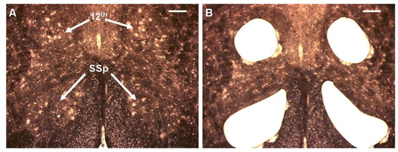
Dehydrated cryosections of adult male zebra finch brainstems mounted on a PEN membrane slide (20x; scale bar, 200 μm). Large motor neurons appear as white cell bodies against a brown neuropil background of axons and dendrites. The 12th and SSp motor nuclei are indicated. (A) Before LCM. (B) After LCM.

Protein Extraction and Digestion

To ensure minimal keratin contamination, perform any sample manipulation before trypsin digestion in a biological safety cabinet or laminar flow hood (i.e., Steps 15–24). See Zhang et al. (2007) for additional information on TFE protein extractions.

• 15Add a 50% (v/v) mixture of 50 mM ammonium bicarbonate and TFE to the glass vial containing the LCM membrane(s) to initiate protein extraction.
• 16Incubate for 10–15 min at 90°C, vortexing several times during extraction.

  TFE will break down plastic vials over time; thus, glass vials are used for this initial step. 

• 17Transfer the supernatant with a pipette to a lo-bind Eppendorf tube.

  The LCM membrane can be discarded. 

• 18Concentrate the supernatant to 10 μL using a vacuum concentrator. Transfer the remaining solution to a glass vial.
• 19Add 1 μL of 100 mM DTT to the solution (i.e., to a final concentration of 10 mM DTT).
• 20Incubate for 15 min at 80°C to reduce the cysteine residues.
• 21Centrifuge any condensation down in a low-speed centrifuge. Cool the solution to room temperature.
• 22Add 1 μL of 200 mM iodoacetamide to the solution (i.e., to a final concentration 20 mM iodoacetamide) to alkylate the cysteine residues. Vortex the solution.
• 23Incubate for 30 min at room temperature.
• 24Add 45 μL of 50 mM ammonium bicarbonate, such that the total concentration of TFE is ≤5%.
• 25Add ~50–100 ng of trypsin such that the ratio of trypsin:total protein is ~1:50.
• 26Incubate with gentle mixing using a thermomixer overnight at 37°C.
• 27Add TFA to a final concentration of 1% (v/v) to acidify the solution and inactivate trypsin.
• 28Vacuum-evaporate the sample to dryness. Resuspend the sample in 25 μ L of 0.1% TFA and 2% acetonitrile.

  The sample is now ready for LC-MS/MS analysis. 

• 29To perform unbiased quantitative proteomic analyses (i.e., label-free comparisons), add 100 fmol of yeast alcohol dehydrogenase digest to each sample as an internal standard for mass spectrometry analyses.

  To determine protein concentration, proceed with Steps 30-35. Otherwise, proceed to Step 36. Protein quantitation is preferred to normalize protein concentrations between samples. However, direct protein concentration measurements can be skipped if insufficient material is available. 

Protein Quantitation

This procedure uses a modification of a commercially available protein assay. A heated-lid PCR thermocycler is used to prevent low-volume sample evaporation, and a NanoDrop spectrophotometer allows for spectroscopic analyses of very small volumes of dilute protein concentrations. Perform the assay on digested protein samples.

• 30Prepare the BCA working solution:

  1. Mix reagents B and C from the kit in a ratio of 25:1 (v/v).

  2. Add reagent A to the B/C mixture in a ratio of 26:1 (v/v).

• 31Prepare 6-7 dilutions (0-0.1 μ g/μ L) of the bovine serum albumin protein standard (provided with the kit as a 2 mg/mL stock solution) in the same buffer as the samples to be assayed.
• 32Add 2 μ L of the protein standards or samples to individually labeled PCR tubes.
• 33Add 2 μ L of the BCA working solution to each protein standard and sample. Mix the contents of each tube by aspirating the solution in a pipette tip.

  See Troubleshooting. 

• 34Incubate the samples in a PCR thermocycler with a heated lid for 30 min at 60°C.
• 35Measure absorbances using the NanoDrop according to the manufacturer’s instructions.

  The NanoDrop BCA application module plots the absorbance of each protein standard as a function of its protein concentration to generate a standard curve (which should be linear from 1 to 100 μg/μL, then uses the standard curve to calculate the protein concentration of the unknowns). 

  1. Open the NanoDrop software on the computer.

  2. Choose the BCA application module.

  3. Initialize the instrument.

  4. Raise the NanoDrop pedestal arm. Place 2 μL of distilled water on the analyzer. Lower the pedestal arm. v. Click "OK" to initialize the instrument.

  5. Blank the instrument using 2 μL of the protein suspension buffer.

  6. Lower the pedestal arm. Click the "blank" button.

     The system is now ready to analyze samples. 

  7. Measure the absorbance of each protein standard and unknown sample at 562 nm by placing 2 μL on the pedestal arm.

LC-MS/MS Data Collection and Processing

Analyze peptide digests from each LCM sample in triplicate using a nanoACQUITY UPLC system coupled to a Synapt HDMS. See Figure 3 for an example of proteomic identification results from the 12th and SSp motor nuclei of male zebra finches as determined by LC-MS/MS.

FIGURE 3.

Qualitative proteomic screening results of the 12th and SSp motor nuclei. (A) Representative reversed-phase HPLC chromatograms of tryptic digests of proteins extracted from the 12th and SSp motor nuclei of one animal. The y-axis indicates the intensity of the peptide signal. The retention time (x-axis) represents the time it takes for a particular peptide to elute from the column and be injected onto the mass spectrometer. (B) Venn diagram showing the differences between the proteomic profiles of the 12th and SSp motor nuclei across six animals.

• 36Separate the peptide fragments:

  1. Load ~250 ng of a digested peptide sample in 8 μL on a 20-μm x 180-mm Symmetry C18 column by running at 20 μL/min for 2 min using water:formic acid (99.9:0.1 [v/v]).

  2. Separate peptide fragments on a 75-μm x 250-mm C18 BEH column using a 90-min gradient of 5%-40% acetonitrile with 0.1% formic acid at a flow rate of 0.3 μL/min and a column temperature of 45°C.

• 37Perform two MS^E analyses per sample for simultaneous peptide quantification and identification

  1. Introduce samples directly into the mass spectrometer via electrospray ionization.

  2. Use a 0.9-sec cycle time, alternating between low-collision energy (6 V) and a high-collision energy ramp (15-40 V).

• 38In addition to quantitative analyses, perform an additional LC-MS/MS analysis in the DDA acquisition mode for each sample for complementary peptide identifications:

  1. Perform a 0.9-sec MS scan.

  2. Perform an MS/MS acquisition on the top three ions with charges >1 using an isolation window of ~3 Da, a maximum of 4 sec per precursor, and dynamic exclusion for 120 sec within 1.2 Da.

LC-MS/MS Data Processing

This method processes LC-MS/MS data using a label-free quantitative pipeline.

• 39Use LC-MS/MS data processing software for raw data alignment, feature identification, and feature extraction. Use the manufacturer’s default settings, with the exception of the lockmass correction.

  The lockmass correction for the quadropole/time-of-flight data is the (M + 2H)²⁺ ion of Glu-Fibrinopeptide B, 785.8426 m/z. See Troubleshooting. 

• 40Use the MS^E and DDA data to generate peptide identifications:

  Set the precursor ion mass tolerance at 20 ppm for both the Mascot and PLGS searches. Use a product ion tolerance of 0.04 Da for Mascot and 40 ppm for PLGS. 

  • For DDA files 

  • iProduce searchable .mgf files using Rosetta Elucidator.
  • iiUse the Mascot v2.2 search engine to search a database of vertebrate proteins (in the example here, including zebra finch) in an automated fashion.

  • For the MS^E data 

  • iiiUse PLGS to generate searchable files using default settings.
• 41Search the DDA and MS^E annotated data against the relevant databases.

  For the example here, data were searched against the NCBInr database (http://www.protein.sdu.dk/gpmaw/GPMAW/Databases/NCBInr/ncbinr.html) containing the zebra finch predicted protein sequences from Ensembl (downloaded March 4, 2009) and the Songbird Brain Transcriptome Database (http://songbirdtranscriptome.net/). The Ensembl and the Songbird Brain Transcriptome databases were modified to contain a full 1x reverse database appended for peptide false discovery rate (FDR) determination. See Wada et al. (2006) and Warren et al. (2010) for additional information on the Jarvis Laboratory transcriptome database and the songbird genome.

• 42Use Protein Digestion Simulator Basic (http://omics.pnl.gov/software/ProteinDigestionSimulatorBasic.php) to remove duplicates from your database of interest. Include carbamidomethyl cysteine as a fixed modification and oxidized methionine as a variable modification.
• 43Import results from your search engines of interest back into Elucidator. Concurrently validate the results with the PeptideTeller and ProteinTeller algorithms using independent decoy database validation and peptides annotated at a 1% peptide FDR.
• 44Add the intensities of peptides annotated to the same protein to gain a measure of the relative protein abundance between samples.

  Use only the MS^E data for quantitative measurements. Because of the way Elucidator aligns data across samples, it uses the same number of peptides for the purpose of quantitation in every sample. 

LC-MS/MS Data Analysis

• 45Normalize signal intensities across peptides (Fig. 4 ):

  1. Obtain the absolute quantity of peptides observed for each Ensembl-predicted protein as determined by the Mascot software tool. Convert all quantities to a log₂ scale to scale fold differences.

  2. Take the subset of data for peptides that are detected in 90% of all samples and whose log₂ median expression is higher than the lower 25th percentile for all data.

  3. Prepare median-centered data by calculating the median log₂ quantity of each peptide. Subtract this value from the log₂ measurements by peptide.

  4. For each sample, calculate the distribution of log₂ median-centered values in 100 steps (such that each step represents one percentage point in the quantile distribution).

  5. Calculate the median profile by taking the median for each step across all samples.

  6. For each sample, calculate the difference from the median profile at each step in the distribution.

  7. Plot each profile using the "steps" as the x-axis and the difference as the y-axis. Confirm that the central regions of each profile are relatively horizontal and log₂ parallel to one another.

     The spread of profiles above and below 1 at the 50th percentile is roughly the effect of the normalization to be applied below. 

  8. Generate a log₂ normalization factor for each sample by taking the mean of the collective 40-60 steps from each sample’s median log₂ differences as plotted above.

  9. Normalize each sample by subtracting the log₂ normalization factor from each log₂ quantity for that sample

     Peptide quantities should now be normalized to a common median reference as defined by the samples being used. 

• 46Use biostatistical methods to compare sample groups using log₂ quantities: the normalized

  1. Use statistical software to perform paired t-tests for each peptide.

  2. Apply a Storey’s Q-value adjustment for each peptide to correct for the presence of many variables (peptides).

• 47Select proteins identified as differentially expressed for validation by immunohistochemistry based on at least two to three criteria.

  When dealing with two tissue regions from the same subject/animal, a paired approach is advised, for example, a paired t-test. If the number of replicates differs between sample groups, an unpaired t-test is advised. When dealing with more than two samples or other variables, an analysis of variance (ANOVA) is advised, assuming the data are normally distributed 

  1. Unadjusted paired t-test P-value <0.01 and Q-value < 0.2

  2. Quantitative differentially expressed proteins replicated in independent experiments (see Fig. 5 )

  3. When multiple peptides are detected, they are differentially expressed in the same direction with similar statistical values.

     This last criterion must be handled with caution because one peptide could be differentially expressed, whereas another representing a different isoform is not. 

FIGURE 4.

Quantitative technical replicate profiles across all samples from one experiment. (A) Raw intensity of technical replicates 1 and 2 from the average LC-MS signal of all peptides in the paired samples of the motor nuclei of each animal. (The SSp sample from Bird 6 was eliminated because protein extraction difficulties resulted in limited protein identifications.) Data points are expressed as mean log₂ intensity. (B) Intensity of each data point normalized to the cross-sample median distribution.

FIGURE 5.

Peptide (LQEYTQTILR) expression profiles of calretinin in the 12th and SSp motor nuclei of male zebra finches. Each value for each nucleus represents the average normalized intensity, identified independently in two separate experiments. Errors bars are the standard error of the mean. (*) Unpaired t-test without (unadj) and with (adj) adjusted FDR P-values.

Biological Validation by Immunohistochemistry

Biological validations can be performed with immunohistochemistry or immunoblots. Immunohistochemistry is useful for determining the number of labeled cells and is the preferred means for secondary screening because it provides anatomical resolution and requires very little tissue (e.g., thin sections). An immunoblot of specific brain regions provides more quantitative information on expression levels and molecular weights, but requires significant amounts of protein. If sufficient material is available, it is useful to perform both.

• 48Perfuse an animal transcardially with PBS for 10 min.
• 49Perfuse the animal transcardially with 4% paraformaldehyde for 30 min.
• 50Dissect the tissue of interest. Postfix in 4% paraformaldehyde for 2 h.
• 51Transfer tissue to a polyethylene tube containing 30% sucrose. Incubate overnight at 4°C.

  The tissue will sink to the bottom of the tube. 

• 52Embed the tissue in a block mold with embedding medium in a dry ice/ethanol bath.
• 53Cut 40-μm sections using a cryostat. Float the sections on PBS in a multiwell plate.

  Tissue-Tek will dissolve in PBS. 

• 54Rinse the sections in PBS three times for 5 min each.
• 55Incubate the sections in a blocking solution of PBS containing 0.3% Triton X and 5% species-specific normal serum for 30 min at room temperature.
• 56Incubate the sections overnight at 4°C in a PBS solution containing 0.3% Triton X and the primary antibody of interest.
• 57The following day, wash the sections in PBS three times for 5 min each.
• 58Incubate the sections in a PBS solution containing the appropriate fluorescent secondary antibody for 2 h at room temperature.
• 59After staining, rinse the tissue in PBS. Mount onto glass slides.
• 60Allow the slides to air-dry. Coverslip the slides with VECTASHIELD.
• 61Observe the immunolabel under a fluorescence microscope to verify and quantify differential expression.

TROUBLESHOOTING

• Problem: In LCM, cells do not adhere to the CapSure cap.

• [Step 14]

• Solution: Ensure that the tissue is properly dehydrated. If the tissue section has folds, try a different section or set the cap in a region away from the folds. Tissue that is folded is not suitable for LCM.

• Problem: Protein unknowns change color rapidly (dark purple) after the addition of BCA working solution.

• [Step 33]

• Solution: Reducing agents such as DTT in concentrations >1 mM interfere with the assay. Dilute the unknowns enough to lower the interference caused by DTT. Be sure to check the effect on the standard curve assayed in the same buffer as the unknown samples.

• Problem: There is polypropylene contamination, denoted by intense +44 Da repeats in the LC-MS/MS chromatograph.

• [Step 39]

• Solution: Limit the amount of time during which the TFE solution is in plastic Eppendorf tubes.

DISCUSSION

Here we developed a comparative microproteomics approach using LCM and gel-free mass spectrometry that can detect and identify hundreds of proteins from fewer than 1000 cells. Relative to high-throughput technologies for assessing gene expression differences between experimental samples (e.g., microarrays, deep sequencing), comparative proteomic technologies are limited by sensitivity and reproducibility (Anderson and Grant 2006; Gutstein et al. 2008). Historically, quantitative proteomic studies have typically relied on two-dimensional difference gel electrophoresis (2D-DIGE) for the separation and visualization of experimental and control samples. 2D-DIGE has been used successfully to detect changes in relative abundance of visualized proteins, various protein isoforms, and post-translational modifications (Merkley et al. 2009; Stephens et al. 2010; Tumani et al. 2010). However, although 2D-DIGE can detect up to approximately 1500 protein spots in a given sample, these spots subsequently must be isolated and identified by a different method, typically mass spectrometry. The disconnect between the expression measurement and protein identification is limited by low throughput, and protein identification is restricted to proteins that show differential expression between two or more states. Also, results can be ambiguous for gel spots where multiple proteins are identified.

Over the last decade, as a complement to gel-based proteomics, several quantitative gel-free proteomic techniques have been developed (Gygi et al. 1999; Olsen et al. 2004; Haqqani et al. 2007). Gel-free approaches use liquid chromatography coupled to tandem mass spectrometry to separate and identify peptides having various physicochemical properties obtained from enzymatic digests of protein extracts, and allows for the simultaneous identification and quantification of proteins. As such, gel-free mass-spectrometry-based techniques have enhanced the range (i.e., the number of protein identifications) and reliability of quantitative proteomic data.

With the advent of LCM, the analytical capabilities of comparative proteomic technologies have improved dramatically. Recently, 2D-DIGE and quantitative gel-free mass spectrometry approaches have been coupled to LCM for proteomic analyses of distinct, pure cell populations (Shekouh et al. 2003; Li et al. 2004; Zang et al. 2004; Haqqani et al. 2005; Bagnato et al. 2007; Mustafa et al. 2008; Patel et al. 2008; Wang et al. 2008; Zhang and Koay 2008; Nan et al. 2009; Scicchitano et al. 2009; Waanders et al. 2009; Yao et al. 2009; Asomugha et al. 2010; Zhang et al. 2010). Other methods such as punch biopsy can be used to microdissect tissues for subsequent proteomic analyses (Folli et al. 2010), but because it is difficult to see the three-dimensional boundaries of structures from the surface of the tissue, punch biopsies can sample adjacent regions that are not of interest. Also, tissues of interest do not necessarily have circular shapes, making punch biopsy less effective. Thus, although tissue obtained from punch biopsy can be used in the protocol presented here, LCM is more precise. Further developments in LCM technology should facilitate effective sampling of specific cellular subtypes from tissue in a high-throughput manner.

Previous studies typically quantified protein expression from tissues containing tens of thousands of cells. The miniaturization of extraction and quantification technologies described here expands the analytical capabilities of comparative proteomics; the procedure is optimized to isolate and detect hundreds of proteins (100-300 proteins) from different cell populations containing as few as 1000 cells. Additionally, it can detect and verify robust protein expression differences between different cell populations (see Fig. 5, Fig.6 ). Unlike traditional proteomic technologies such as SDS-PAGE with mass spectrometry identification or 2D-DIGE, which require at least 10–50 μg of protein (Sloley et al. 2007; Pinaud et al. 2008), this procedure requires 1–2 μg of protein. However, each step of the procedure requires greater care as the sample size decreases. Protein losses during extraction and separation become more significant as the protein detection limit (<0.75 μg) is approached. It also becomes more difficult to evaluate differences between two samples with small amounts of protein because the variability increases as one operates closer to the limits of detection of the analytical technique. Our technique addresses the quantitation issues associated with very small protein concentrations. Although commercially available protein assays can reliably quantify concentrations ranging from 20 to 2000 μg/μL, they often require large volumes of concentrated protein samples. The modified procedure described here can reliably quantify small volumes of dilute protein concentrations in the 1–100 μg/μL range.

FIGURE 6.

Immunohistochemical validation of calretinin expression in the 12th and SSp motor nuclei. (A) Darkfield coronal section of male zebra finch brainstem. (B) The same section as in A under fluorescence imaging shows calretinin expression (green) detected by a fluorescein isothiocyanate (FITC)-labeled calretinin-specific antibody. (C) Quantitative analysis of calretinin- expressing cells. The total number of motor neurons was determined from darkfield images; the number of calretinin-labeled neurons was determined from FITC fluorescence images. There are nine times as many calretinin-positive neurons in the SSp motor nucleus as there are in the 12th motor nucleus (n = 3; [*] p < 0.003). Scale bars, 500 μm.

In the example presented here, this protocol was used to screen for proteomic differences potentially involved in vocal learning in songbirds. Vocal learning is the ability to acquire vocalizations through imitation and is a critical behavioral substrate for spoken human language (Jarvis 2004). Molecular differences at the protein level might control the maintenance of the forebrain-to-brainstem projection in vocal learning avian species. The 12th motor nucleus controls the syrinx muscles and receives a direct forebrain projection in vocal learning species (e.g., songbirds, parrots, hummingbirds) (Jarvis 2004), whereas the SSp motor nucleus controls the neck muscles and does not receive a direct forebrain projection in either vocal learner or vocal nonlearner avian species. Similar findings have been demonstrated in mammals, including vocal learning humans versus vocal nonlearning nonhuman primates (Jarvis 2004; Jürgens 2009). A comparison of the proteomic differences between these nuclei from six adult male zebra finches identified and quantified 245 proteins. Future work will involve manipulation of the differentially regulated proteins.

References

- 1.Anderson CNG, Grant SGN. High throughput protein expression screening in the nervous system: Needs and limitations. J Physiol. 2006;575:367–372. doi: 10.1113/jphysiol.2006.113795. [Abstract/Free Full Text] [DOI] [PMC free article] [PubMed] [Google Scholar]
- 2.Asomugha CO, Gupta R, Srivastava OP. Identification of crystallin modifications in the human lens cortex and nucleus using laser capture microdissection and CyDye labeling. Mol Vis. 2010;16:476–494. [PMC free article] [PubMed] [Google Scholar]
- 3.Bagnato C, Thumar J, Mayya V, Hwang S-I, Zebroski H, Claffey KP, Haudenschild C, Eng JK, Lundgren DH, Han DK. Proteomics analysis of human coronary atherosclerotic plaque: A feasibility study of direct tissue proteomics by liquid chromatography and tandem mass spectrometry. Mol Cell Proteomics. 2007;6:1088–1102. doi: 10.1074/mcp.M600259-MCP200. [Abstract/Free Full Text] [DOI] [PubMed] [Google Scholar]
- 4.Carducci C, Birarelli M, Santagata P, Leuzzi V, Carducci C, Antonozzi I. Automated high-performance liquid chromatographic method for the determination of guanidinoacetic acid in dried blood spots: A tool for early diagnosis of guanidinoacetate methyltransferase deficiency. J Chromatogr B Biomed Sci Appl. 2001;755:343–348. doi: 10.1016/s0378-4347(01)00052-4. [DOI] [PubMed] [Google Scholar]
- 5.Cox J, Mann M. MaxQuant enables high peptide identification rates, individualized p.p.b.-range mass accuracies and proteome-wide protein quantification. Nat Biotechnol. 2008;26:1367–1372. doi: 10.1038/nbt.1511. [DOI] [PubMed] [Google Scholar]
- 6.Cui DP, Dougherty KJ, Machacek DW, Sawchuk M, Hochman S, Baro DJ. Divergence between motoneurons: Gene expression profiling provides a molecular characterization of functionally discrete somatic and autonomic motoneurons. Physiol Genomics. 2006;24:276–289. doi: 10.1152/physiolgenomics.00109.2005. [Abstract/Free Full Text] [DOI] [PMC free article] [PubMed] [Google Scholar]
- 7.Espina V, Wulfkuhle JD, Calvert VS, VanMeter A, Zhou W, Coukos G, Geho DH, Petricoin EF, III, Liotta LA. Laser-capture microdissection. Nat Protoc. 2006;1:586–603. doi: 10.1038/nprot.2006.85. [DOI] [PubMed] [Google Scholar]
- 8.Folli F, Guzzi V, Perego L, Coletta DK, Finzi G, Placidi C, La Rosa S, Capella C, Socci C, Lauro D, et al. Proteomics reveals novel oxidative and glycolytic mechanisms in type 1 diabetic patients’ skin which are normalized by kidney-pancreas transplantation. PLoS One. 2010;5:e9923. doi: 10.1371/journal.pone.0009923. [DOI] [PMC free article] [PubMed] [Google Scholar]
- 9.Geromanos SJ, Vissers JPC, Silva JC, Dorschel CA, Li G-Z, Gorenstein MV, Bateman RH, Langridge JI. The detection, correlation, and comparison of peptide precursor and product ions from data independent LC-MS with data dependent LC-MS/MS. Proteomics. 2009;9:1683–1695. doi: 10.1002/pmic.200800562. [DOI] [PubMed] [Google Scholar]
- 10.Gutstein HB, Morris JS. Laser capture sampling and analytical issues in proteomics. Expert Rev Proteomics. 2007;4:627–637. doi: 10.1586/14789450.4.5.627. [DOI] [PMC free article] [PubMed] [Google Scholar]
- 11.Gutstein HB, Morris JS, Annangudi SP, Sweedler JV. Microproteomics: Analysis of protein diversity in small samples. Mass Spectrom Rev. 2008;27:316–330. doi: 10.1002/mas.20161. [DOI] [PMC free article] [PubMed] [Google Scholar]
- 12.Gygi SP, Rist B, Gerber SA, Turecek F, Gelb MH, Aebersold R. Quantitative analysis of complex protein mixtures using isotope-coded affinity tags. Nat Biotechnol. 1999;17:994–999. doi: 10.1038/13690. [DOI] [PubMed] [Google Scholar]
- 13.Haqqani AS, Nesic M, Preston E, Baumann E, Kelly J, Stanimirovic D. Characterization of vascular protein expression patterns in cerebral ischemia/reperfusion using laser capture microdissection and ICAT-nanoLC-MS/MS. FASEB J. 2005;19:1809–1821. doi: 10.1096/fj.05-3793com. [Abstract/Free Full Text] [DOI] [PubMed] [Google Scholar]
- 14.Haqqani AS, Kelly J, Baumann E, Haseloff RF, Blasig IE, Stanimirovic DB. Protein markers of ischemic insult in brain endothelial cells identified using 2D gel electrophoresis and ICAT-based quantitative proteomics. J Proteome Res. 2007;6:226–239. doi: 10.1021/pr0603811. [DOI] [PubMed] [Google Scholar]
- 15.Jaffe JD, Mani DR, Leptos KC, Church GM, Gillette MA, Carr SA. PEPPeR, a platform for experimental proteomic pattern recognition. Mol Cell Proteomics. 2006;5:1927–1941. doi: 10.1074/mcp.M600222-MCP200. [Abstract/Free Full Text] [DOI] [PMC free article] [PubMed] [Google Scholar]
- 16.Jarvis ED. Learned birdsong and the neurobiology of human language. Ann N Y Acad Sci. 2004;1016:749–777. doi: 10.1196/annals.1298.038. [DOI] [PMC free article] [PubMed] [Google Scholar]
- 17.Jürgens U. The neural control of vocalization in mammals: A review. J Voice. 2009;23:1–10. doi: 10.1016/j.jvoice.2007.07.005. [DOI] [PubMed] [Google Scholar]
- 18.Kiebel GR, Auberry KJ, Jaitly N, Clark DA, Monroe ME, Peterson ES, Tolić N, Anderson GA, Smith RD. PRISM: A data management system for high-throughput proteomics. Proteomics. 2006;6:1783–1790. doi: 10.1002/pmic.200500500. [DOI] [PubMed] [Google Scholar]
- 19.Kislinger T, Rahman K, Radulovic D, Cox B, Rossant J, Emili A. PRISM, a generic large scale proteomic investigation strategy for mammals. Mol Cell Proteomics. 2003;2:96–106. doi: 10.1074/mcp.M200074-MCP200. [Abstract/Free Full Text] [DOI] [PubMed] [Google Scholar]
- 20.Li C, Hong Y, Tan Y-X, Zhou H, Ai J-H, Li S-J, Zhang L, Xia Q-C, Wu J-R, Wang H-Y, et al. Accurate qualitative and quantitative proteomic analysis of clinical hepatocellular carcinoma using laser capture microdissection coupled with isotope-coded affinity tag and two-dimensional liquid chromatography mass spectrometry. Mol Cell Proteomics. 2004;3:399–409. doi: 10.1074/mcp.M300133-MCP200. [Abstract/Free Full Text] [DOI] [PubMed] [Google Scholar]
- 21.Li G-Z, Vissers JPC, Silva JC, Golick D, Gorenstein MV, Geromanos SJ. Database searching and accounting of multiplexed precursor and product ion spectra from the data independent analysis of simple and complex peptide mixtures. Proteomics. 2009;9:1696–1719. doi: 10.1002/pmic.200800564. [DOI] [PubMed] [Google Scholar]
- 22.Melle C, Ernst G, Grosheva M, Angelov DN, Irintchev A, Guntinas-Lichius O, von Eggeling F. Proteomic analysis of microdissected facial nuclei of the rat following facial nerve injury. J Neurosci Methods. 2009;185:23–28. doi: 10.1016/j.jneumeth.2009.09.003. [DOI] [PubMed] [Google Scholar]
- 23.Merkley MA, Weinberger PM, Jackson LL, Podolsky RH, Lee JR, Dynan WS. 2D-DIGE proteomic characterization of head and neck squamous cell carcinoma. Otolaryngol Head Neck Surg. 2009;141:626–632. doi: 10.1016/j.otohns.2009.08.011. [DOI] [PMC free article] [PubMed] [Google Scholar]
- 24.Mustafa D, Kros JM, Luider T. Combining laser capture microdissection and proteomics techniques. Methods Mol Biol. 2008;428:159–178. doi: 10.1007/978-1-59745-117-8_9. [DOI] [PubMed] [Google Scholar]
- 25.Nan Y, Yang S, Tian Y, Zhang W, Zhou B, Bu L, Huo S. Analysis of the expression protein profiles of lung squamous carcinoma cell using shot-gun proteomics strategy. Med Oncol. 2009;26:215–221. doi: 10.1007/s12032-008-9109-4. [DOI] [PubMed] [Google Scholar]
- 26.Neubert H, Bonnert TP, Rumpel K, Hunt BT, Henle ES, James IT. Label-free detection of differential protein expression by LC/MALDI mass spectrometry. J Proteome Res. 2008;7:2270–2279. doi: 10.1021/pr700705u. [DOI] [PubMed] [Google Scholar]
- 27.Olsen JV, Andersen JR, Nielsen PA, Nielsen ML, Figeys D, Mann M, Wiśniewski JR. HysTag—A novel proteomic quantification tool applied to differential display analysis of membrane proteins from distinct areas of mouse brain. Mol Cell Proteomics. 2004;3:82–92. doi: 10.1074/mcp.M300103-MCP200. [Abstract/Free Full Text] [DOI] [PubMed] [Google Scholar]
- 28.Paša-Tolić L, Masselon C, Barry RC, Shen YF, Smith RD. Proteomic analyses using an accurate mass and time tag strategy. Biotechniques. 2004;37:621–639. doi: 10.2144/04374RV01. [DOI] [PubMed] [Google Scholar]
- 29.Patel V, Hood BL, Molinolo AA, Lee NH, Conrads TP, Braisted JC, Krizman DB, Veenstra TD, Gutkind JS. Proteomic analysis of laser-captured paraffin-embedded tissues: A molecular portrait of head and neck cancer progression. Clin Cancer Res. 2008;14:1002–1014. doi: 10.1158/1078-0432.CCR-07-1497. [Abstract/Free Full Text] [DOI] [PubMed] [Google Scholar]
- 30.Pinaud R, Osorio C, Alzate O, Jarvis ED. Profiling of experience-regulated proteins in the songbird auditory forebrain using quantitative proteomics. Eur J Neurosci. 2008;27:1409–1422. doi: 10.1111/j.1460-9568.2008.06102.x. [DOI] [PMC free article] [PubMed] [Google Scholar]
- 31.Scicchitano MS, Dalmas DA, Boyce RW, Thomas HC, Frazier KS. Protein extraction of formalin-fixed, paraffin-embedded tissue enables robust proteomic profiles by mass spectrometry. J Histochem Cytochem. 2009;57:849–860. doi: 10.1369/jhc.2009.953497. [Abstract/Free Full Text] [DOI] [PMC free article] [PubMed] [Google Scholar]
- 32.Shekouh AR, Thompson CC, Prime W, Campbell F, Hamlett J, Herrington CS, Lemoine NR, Crnogorac-Jurcevic T, Buechler MW, Friess H, et al. Application of laser capture microdissection combined with two-dimensional electrophoresis for the discovery of differentially regulated proteins in pancreatic ductal adenocarcinoma. Proteomics. 2003;3:1988–2001. doi: 10.1002/pmic.200300466. [DOI] [PubMed] [Google Scholar]
- 33.Silva JC, Denny R, Dorschel CA, Gorenstein M, Kass IJ, Li G-Z, McKenna T, Nold MJ, Richardson K, Young P, et al. Quantitative proteomic analysis by accurate mass retention time pairs. Anal Chem. 2005;77:2187–2200. doi: 10.1021/ac048455k. [DOI] [PubMed] [Google Scholar]
- 34.Silva JC, Denny R, Dorschel C, Gorenstein MV, Li G-Z, Richardson K, Wall D, Geromanos SJ. Simultaneous qualitative and quantitative analysis of the Escherichia coli proteome: A sweet tale. Mol Cell Proteomics. 2006;5:589–607. doi: 10.1074/mcp.M500321-MCP200. [Abstract/Free Full Text] [DOI] [PubMed] [Google Scholar]
- 35.Sloley S, Smith S, Gandhi S, Busby JAC, London S, Luksch H, Clayton DF, Bhattacharya SK. Proteomic analyses of zebra finch optic tectum and comparative histochemistry. J Proteome Res. 2007;6:2341–2350. doi: 10.1021/pr070126w. [DOI] [PubMed] [Google Scholar]
- 36.Smith RD, Anderson GA, Lipton MS, Paša-Tolić L, Shen YF, Conrads TP, Veenstra TD, Udseth HR. An accurate mass tag strategy for quantitative and high-throughput proteome measurements. Proteomics. 2002;2:513–523. doi: 10.1002/1615-9861(200205)2:5<513::AID-PROT513>3.0.CO;2-W. [DOI] [PubMed] [Google Scholar]
- 37.Stephens AN, Hannan NJ, Rainczuk A, Meehan KL, Chen J, Nicholls PK, Rombauts LJF, Stanton PG, Robertson DM, Salamonsen LA. Post-translational modifications and protein-specific isoforms in endometriosis revealed by 2D DIGE. J Proteome Res. 2010;9:2438–2449. doi: 10.1021/pr901131p. [DOI] [PubMed] [Google Scholar]
- 38.Tolmachev AV, Monroe ME, Purvine SO, Moore RJ, Jaitly N, Adkins JN, Anderson GA, Smith RD. Characterization of strategies for obtaining confident identifications in bottom-up proteomics measurements using hybrid FTMS instruments. Anal Chem. 2008;80:8514–8525. doi: 10.1021/ac801376g. [DOI] [PMC free article] [PubMed] [Google Scholar]
- 39.Tumani H, Lehmensiek V, Lehnert S, Otto M, Brettschneider J. 2D DIGE of the cerebrospinal fluid proteome in neurological diseases. Expert Rev Proteomics. 2010;7:29–38. doi: 10.1586/epr.09.99. [DOI] [PubMed] [Google Scholar]
- 40.Waanders LF, Chwalek K, Monetti M, Kumar C, Lammert E, Mann M. Quantitative proteomic analysis of single pancreatic islets. Proc Natl Acad Sci. 2009;106:18902–18907. doi: 10.1073/pnas.0908351106. [Abstract/Free Full Text] [DOI] [PMC free article] [PubMed] [Google Scholar]
- 41.Wada K, Howard JT, McConnell P, Whitney O, Lints T, Rivas MV, Horita H, Patterson MA, White SA, Scharff C, et al. A molecular neuroethological approach for identifying and characterizing a cascade of behaviorally regulated genes. Proc Natl Acad Sci. 2006;103:15212–15217. doi: 10.1073/pnas.0607098103. [Abstract/Free Full Text] [DOI] [PMC free article] [PubMed] [Google Scholar]
- 42.Wang Z, Han J, Schey KL. Spatial differences in an integral membrane proteome detected in laser capture microdissected samples. J Proteome Res. 2008;7:2696–2702. doi: 10.1021/pr700737h. [DOI] [PMC free article] [PubMed] [Google Scholar]
- 43.Warren WC, Clayton DF, Ellegren H, Arnold AP, Hillier LW, Künstner A, Searle S, White S, Vilella AJ, Fairley S, et al. The genome of a songbird. Nature. 2010;464:757–762. doi: 10.1038/nature08819. [DOI] [PMC free article] [PubMed] [Google Scholar]
- 44.Yao H, Zhang Z, Xiao Z, Chen Y, Li C, Zhang P, Li M, Liu Y, Guan Y, Yu Y, et al. Identification of metastasis associated proteins in human lung squamous carcinoma using two-dimensional difference gel electrophoresis and laser capture microdissection. Lung Cancer. 2009;65:41–48. doi: 10.1016/j.lungcan.2008.10.024. [DOI] [PubMed] [Google Scholar]
- 45.Zang L, Palmer-Toy D, Hancock WS, Sgroi DC, Karger BL. Proteomic analysis of ductal carcinoma of the breast using laser capture microdissection, LC-MS, and 16 O/18O isotopic labeling. J Proteome Res. 2004;3:604–612. doi: 10.1021/pr034131l. [DOI] [PubMed] [Google Scholar]
- 46.Zhang D, Koay ES. Analysis of laser capture microdissected cells by 2-dimensional gel electrophoresis. Methods Mol Biol. 2008;428:77–91. doi: 10.1007/978-1-59745-117-8_5. [DOI] [PubMed] [Google Scholar]
- 47.Zhang H, Lin Q, Ponnusamy S, Kothandaraman N, Lim TK, Zhao C, Kit HS, Arijit B, Rauff M, Hew C-L, et al. Differential recovery of membrane proteins after extraction by aqueous methanol and trifluoroethanol. Proteomics. 2007;7:1654–1663. doi: 10.1002/pmic.200600579. [DOI] [PubMed] [Google Scholar]
- 48.Zhang Y, Ye Y, Shen D, Jiang K, Zhang H, Sun W, Zhang J, Xu F, Cui Z, Wang S. Identification of transgelin-2 as a biomarker of colorectal cancer by laser capture microdissection and quantitative proteome analysis. Cancer Sci. 2010;101:523–529. doi: 10.1111/j.1349-7006.2009.01424.x. [DOI] [PMC free article] [PubMed] [Google Scholar]