Characterizing and Differentiating Brain State Dynamics via Hidden Markov Models

Abstract

Functional connectivity measured from resting state fMRI (R-fMRI) data has been widely used to examine the brain’s functional activities and has been recently used to characterize and differentiate brain conditions. However, the dynamical transition patterns of the brain’s functional states have been less explored. In this work, we propose a novel computational framework to quantitatively characterize the brain state dynamics via hidden Markov models (HMMs) learned from the observations of temporally dynamic functional connectomics, denoted as functional connectome states. The framework has been applied to the R-fMRI dataset including 44 post-traumatic stress disorder (PTSD) patients and 51 normal control (NC) subjects. Experimental results show that both PTSD and NC brains were undergoing remarkable changes in resting state and mainly transiting amongst a few brain states. Interestingly, further prediction with the best-matched HMM demonstrates that PTSD would enter into, but could not disengage from, a negative mood state. Importantly, 84 % of PTSD patients and 86 % of NC subjects are successfully classified via multiple HMMs using majority voting.

Introduction

The brain’s functional connectivity constructed via neuroimaging data such as resting state fMRI (R-fMRI) has attracted many researchers’ attention in recent years. Functional connectivity not only offers a macroscopic description of the functional segregation and integration within the brain (Sporns et al. 2005; Williams 2010; Kennedy 2010; Biswal et al. 2010; Dijk et al. 2010; Hagmann et al. 2010), but also can be used to characterize and differentiate brain conditions (Lynall et al. 2010; Li et al. 2013a; Dickerson and Sperling 2009; Stebbins and Murphy 2009; Liang et al. 2011; Binnewijzend et al. 2012). In many previous R-fMRI based connectivity studies (Lynall et al. 2010; Dickerson and Sperling 2009; Zhang et al. 2013), the functional connectivity or connectome has been widely assumed to be temporally stationary, that is, the whole scan session’s R-fMRI data is used for measuring the functional connectivity or connectome. However, there are growing evidences (Li et al. 2013b; Chang and Glover 2010; Smith et al. 2012; Li et al. 2014; Gilbert and Sigman 2007) indicating that functional brain activities are under temporally dynamic changes at different time scales. At a basic level, recent neuroscience studies suggested that the functional activity of any cortical area is subject to top-down influences of attention, expectation, and perceptual tasks (Gilbert and Sigman 2007). For instance, each cortical brain area runs different “programs” according to the context and to the current perceptual requirements (Gilbert and Sigman 2007). Specially, the dynamically changing functional interactions among structural connections from higher- to lower-order brain areas and intrinsic cortical circuits mediate the moment-by-moment functional state changes in the brain (Gilbert and Sigman 2007). Brain is still very active in resting state, due to the unconstrained behaviors or conscious mentations, which might include mind wandering, visual imagery and etc. (Fox and Raichle 2007). Therefore, the functional brain connectivity is still undergoing considerable dynamic changes within time scales of seconds to minutes (Li et al. 2013b; Chang and Glover 2010; Smith et al. 2012; Li et al. 2014; Gilbert and Sigman 2007) in resting state, and that dynamic changes in connectivity cannot be ignored when analyzing brain connectivity in resting state.

Recently, neuroscience and neuroimaging researchers have begun to study the brain’s functional dynamics based on functional connectivities/connectomics (Li et al. 2013b; Chang and Glover 2010; Smith et al. 2012; Li et al. 2014; Gilbert and Sigman 2007; Bassett et al. 2011; Ekman et al. 2012). For instance, Li et al. (Li et al. 2014) modeled the moment-by-moment functional state switching in the brain by a finite state machine (FSM) in their work. However, the FSM in Li et al. (Li et al. 2014) is limited to describe the temporally dynamic transition patterns of the brain’s functional connectivities, and it hasn’t quantitatively characterized the intrinsic stochastic relationships among those temporally dynamic brain states. It is important to note that Eavani et al. (Eavani et al. 2013) utilized HMM to learn the dynamic functional connectivity networks with the observations of the R-fMRI time series. While in this work, we aim to model the dynamics of functional brain states (FBSs) with the observations of the dynamical functional connectomes. Given that R-fMRI is an indirect measurement of the brain’s function (Biswal 2012; Richiardi et al. 2011), it is reasonable to postulate that the true brain state is not directly visible, but the R-fMRI derived functional connectomics that are dependent on the true brain states are visible. Therefore, in this work, we employ the powerful methods of HMMs to characterize and analyze the hidden brain states and their temporally dynamic transition patterns in the brain based on R-fMRI derived functional connectomics.

Motivated by the dynamic transition patterns of the brain’s functional connectomics (Li et al. 2014) and inspired by indirect measurement of the FBSs by using functional connectomes (Biswal 2012; Richiardi et al. 2011), in this work, we propose a novel computational framework to stochastically characterize the dynamic transition patterns of the FBSs via HMMs learned from the dynamical functional connectomes, which are derived via a sliding time window approach (Allen et al. 2012; Li et al. 2014). Here, our recently developed and publicly released 358 DICCCOL (Dense Individualized and Common Connectivity based Cortical Landmarks) landmarks (Zhu et al. 2013) are employed as the network nodes for connectivity mapping. The neuroscience basis is the “connectional fingerprint”, that is, each cytoarchitectonic area possesses a unique set of extrinsic inputs and outputs, which largely determine the functions that the area can perform (Passingham et al. 2002). Each DICCCOL is optimized to possess maximal group-wise consistency of DTI-derived fiber shape patterns (Zhu et al. 2013). Therefore, those DICCCOLs possess intrinsically-established structural and functional correspondences across different individuals and populations, and offer a generic brain reference system for integrating and comparing function connectomes across individuals and populations. The applicability of the computational framework has been demonstrated by applying it to the R-fMRI dataset of 44 PTSD patients and 51 NC subjects. Experimental results have suggested that both PTSD and NC brains were undergoing remarkably dynamical changes and mainly transiting amongst several brain states. Interestingly, further prediction with the best-matched HMM for PTSD demonstrates that PTSD would enter into, and could not disengage from, a negative mood state (Holtzheimer and Mayberg 2011). Moreover, we treated the combination of any two HMMs, one from NC and the other from PTSD, as a classifier for classifying PTSD patients from NC subjects. Results demonstrated that 84 % of PTSD patients and 86 % of NC subjects were successfully classified via multiple classifiers with majority voting (Ruta and Gabrys 2005; Kittler et al. 1998).

Conceptually, the major methodological contributions of this work are two folds. First, the adopted HMM provides an effective probabilistic modeling framework to stochastically characterize the hidden FBSs inferred from the observed time-varying functional connectomics in the fMRI data. The HMMs learned from the R-fMRI data can offer insights into the functional dynamics of the brain. Second, the application of the HMMs in a multimodal PTSD dataset has identified important and meaningful phenomena and principles, which could not be revealed by our previous studies (Li et al. 2014). In particular, the HMMs can be potentially used as neuroimaging biomarkers for differentiation and classification of PTSD patients in the future. The rest of the paper is organized as follows. “Materials and Methods” section details the dataset and the modeling methods including FCS construction and HMM inference. Experimental results on a multimodal DTI/R-fMRI PTSD dataset and their neuroscience interpretation are presented in “Results” section. “Discussion and Conclusion” section provides discussions on limitations and future direction of this work, and concludes this work. Notably, an early abstract of this methodology on ADHD data was presented in the 2013 IEEE EMBS conference on Neural Engineering (Jinli et al. 2013).

Materials and Methods

Overview

The computational framework is composed of three main parts and seven steps, as summarized in Fig. 1. The three main components are: Step 1: functional connectome state (FCS) construction from the R-fMRI dataset; Steps 2–5: HMM modeling including FCS clustering, HMM learning and HMM decoding; Step 6–7: PTSD classification including FCS labeling and PTSD classification via multiple HMMs using majority voting. Details of these three main parts and seven steps will be described in details in the following sections.

Fig. 1.

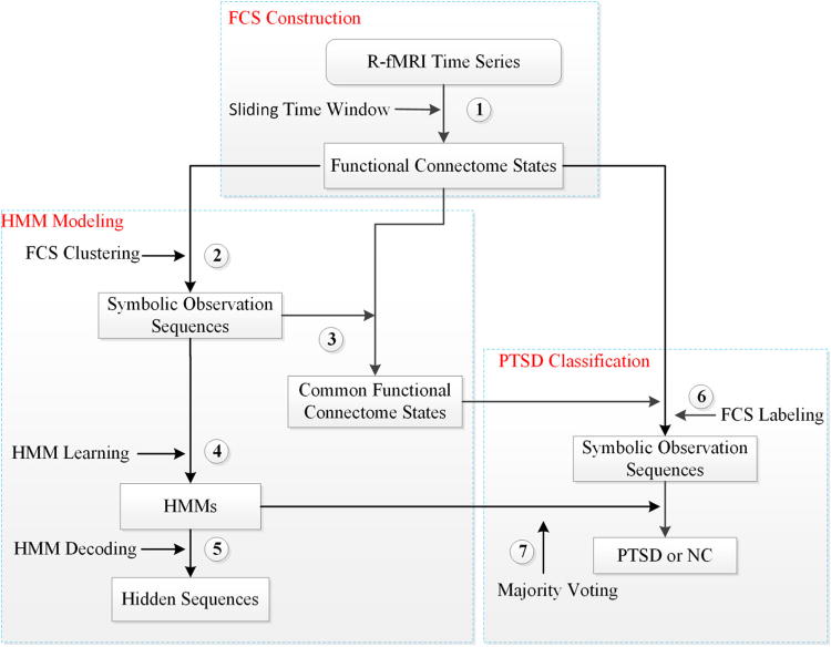
Block diagram of the computational framework composed of three main parts and seven steps. (1) FCS construction via a sliding time window on the R-fMRI time series signals; (2) The symbolic observation sequences generation via a two-stage hierarchical clustering i.e., FCS clustering; (3) The CFCS derivation via calculating the average of those FCSs belonging to the same cluster after FCS clustering; (4) HMM learning based on the symbolic observation sequences; (5) The symbolic hidden sequences decoding from the two best-matched HMMs for NC and PTSD; (6) FCS labeling based on the Euclidean distance between the FCS and CFCSs; (7) Classification of PTSD patients from NC subjects via multiple HMMs using majority voting

Data Acquisition and Preprocessing

We used the DTI and R-fMRI datasets of 95 adult subjects including 44 PTSD patients and 51 NC subjects (Li et al. 2014). The datasets were acquired using a 3T GE MRI scanner in West China Hospital, Huaxi MR Research Center, Department of Radiology, Chengdu, China, under IRB approvals, with the following parameters. R-fMRI: number of slices, 30; matrix size, 64 × 64; slice thickness, 4 mm; field of view (FOV), 220 mm; repetition time (TR), 2 s; total scan time, 400 s. DTI: number of slices, 50; matrix size, 256 × 256; slice thickness, 3 mm; field of view (FOV), 240 mm; DWI volumes, 15; b-value, 1000.

The preprocessing steps for multimodal DTI and R-fMRI datasets can be found in our previous publications (Zhu et al. 2013). After preprocessing, the 358 consistent DICCCOL landmarks, which have been proved to be consistent and reproducible over 240 brains and provide the structural substrates for functional connectome mapping, are predicted in the DTI data via maximizing the group-wise consistency of white fiber connection patterns. Briefly, DICCCOL prediction consists of three steps: the initial landmarks selection, the optimization of landmark locations and the determination of group-wise consistent DICCCOLs (Zhu et al. 2013). Then we co-register the R-fMRI images into the DTI space using FSL FLIRT. At last, the R-fMRI BOLD time series are extracted by averaging in a small neighborhood (3 mm radius) for each DICCCOL.

Functional Connectome State Construction

The FBS is indirectly characterized by a large-scale functional connectivity matrix, denoted as functional connectome state (FCS). The pairwise functional connectivity is defined as the Pearson correlations between the windowed R-fMRI time series signals extracted from any two nodes out of the 358 DICCCOL ROIs (regions of interest). In order to capture the dynamics of FCSs, a sliding time window approach (Li et al. 2013b, 2014; Allen et al. 2012) was applied to segment the R-fMRI time series X_i from the i-th DICCCOL into temporal segments TS_i,t at the time point t, with the window length l:

$$T{S}_{i,t}=\{X_{i,pt}|t\le pt<t+l\},$$ (1)

where X_i,pt is the value of R-fMRI time series X_i at time point pt. Since we have already achieved relative good FSMs to describe FCS transition patterns with the window length of 14 in our previous study (Li et al. 2014), the window length l is also set as 14 in this work. Then, the functional connectivity between the i-th and j-th DICCCOLs at time point t can be evaluated as the Pearson correlation R_i,j,t between the segments TS_i,t and TS_j,t:

$$R_{i,j,t}=\mathrm{corr}(T{S}_{i,t},T{S}_{j,t});FC{S}_t=\{R_{i,j,t}|i,j\in (1,358)\}$$ (2)

Thus, each FCS is characterized by a 358 × 358 symmetrical functional connectivity matrix. To have a compact representation of FCS, we defined the cumulative functional connectivity strength (FCS_stre) to represent FCS for computation purpose:

$$FC{S}_{\mathit{stre}}={\displaystyle \sum _1^{358}}{R}_{i,j,t}$$ (3)

Therefore, the FCS (358 × 358) matrix is converted into a representative connectivity vector (358 × 1), and thus each FCS has a connectivity matrix representation and a compact connectivity strength representation. Because of the intrinsically established correspondences of the DICCCOL landmarks across individual brains (Zhu et al. 2013), the FCSs in different windows and across different brains can be readily pooled and integrated for further processing. An example of the FCS construction and its dynamics transition pattern is illustrated in Fig. 2. As the time window sliding, the dynamic FCS transition pattern of each subject is captured.

Fig. 2.

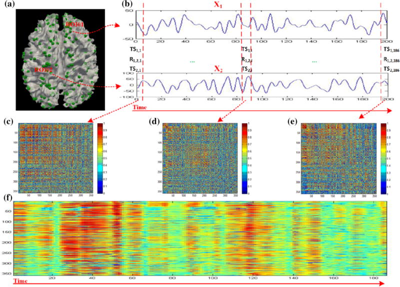
Demonstration of functional connectome state (FCS) construction with the sliding time window. a Visualization of the publicly available 358 DICCCOL landmarks with two randomly selected ROIs, named ROI#1 and ROI#2. b R-fMRI time series signals, named X₁ and X₂, extracted from ROI#1 and ROI#2 respectively. c–e Visualization of the functional connectivities within the three time windows marked by red dotted lines in b color-coded by their correlation value. f Visualization of temporally varying patterns of FCSs

HMM Modeling Based on Temporally Dynamic FCSs

Briefly, the modeling algorithm contains the following two steps: FCS clustering and HMM learning. In order to learn two independent HMM sets for NC and PTSD respectively for characterization and differentiation PTSD patients from NC subjects, the dataset is divided into two independent subsets, one including all the NC subjects, the other including all the PTSD patients.

FCS Clustering

In this work, FCS is considered as an indirect measurement of brain state. Different FCSs in different time windows and across different individuals may indirectly measure the same brain state. In order to identify those FCSs which indirectly measure the same brain state and label them with the same symbolic observation state, we applied the hierarchical clustering based on the average link method (Murtagh 1983; Jain et al. 1999) to the FCS sequences of NC and PTSD. Then the symbolic observation sequences corresponding to the FCS sequences are obtained (Fig. 2f), based on which we learn the HMMs (Rabiner 1989; Stratonovich 1960). Hierarchical clustering is a non-parametric and effective method to classify the brain’s functional connectivity (Cordes et al. 2002; Li et al. 2009) and assumes very little in the way of data characteristics or of a priori knowledge on the part of the analysis (Murtagh 1983). In this work, the distance between FCSs is measured via the Euclidean distance between them (Jain et al. 1999; Cordes et al. 2002).

In our dataset, there are 51 NC subjects and 44 PTSD patients, each subject has 186 FCSs obtained by using the sliding time window length of 14 (Li et al. 2013b, 2014). The sliding time window length was determined experimentally and it has been shown in our previous work (Li et al. 2014) that within a reasonable range, the connectivity and its dynamics would not be affected by the choice of the length value. Totally, there are 9486 FCSs for NC and 8184 FCSs for PTSD. As a result, the distance matrices in the hierarchical clustering are relatively huge, with the dimensions of 9,486 × 9,486 for NC and 8,184 × 8,184 for PTSD. Due to the limited computating resources, we adopted a two-stage hierarchical clustering approach. At first stage, we applied the hierarchical clustering on the individual 186 FCSs of each subject (Fig. 3a). Then the average of those FCSs which belong to the same cluster is calculated, denoted as FCSC (FCS cluster):

$$\mathit{FCSC}=\frac{1}{N_i}{\displaystyle \sum _{{\mathit{FCS}}_t\in {\mathit{cluster}}_i}}{\mathit{FCS}}_t$$ (4)

here N_i is the number of FCSs within the cluster i. After the first-stage hierarchical clustering, the number of FCSs is reduced to the total number of clusters in each subject. Subsequently, we applied the hierarchical clustering to the two collections of FCSCs of NC and PTSD separately (Fig. 3b), and the average of the clusters are calculated again, named as common FCSs (CFCSs). Since each FCS has a connectivity matrix representation and a compact connectivity strength representation, we can also derive a connectivity matrix representation and a compact connectivity strength representation for each CFCS. (During the hierarchical clustering, we utilized the compact connectivity strength representation of FCS.)

Fig. 3.

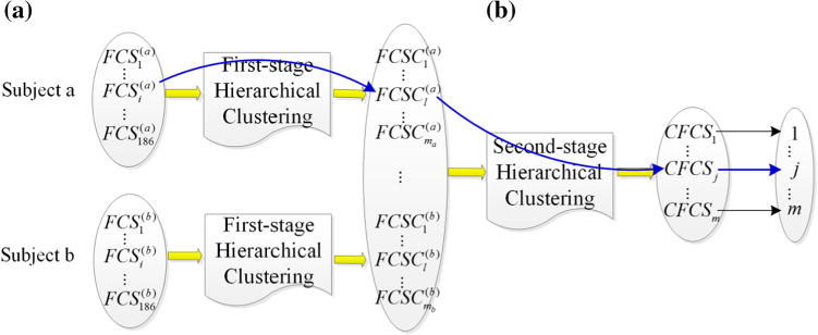
Demonstration of FCS clustering. The FCS clustering contains two clustering steps: a The first-stage hierarchical clustering on the individual 186 FCSs of each subject. b The second-stage hierarchical clustering on all the averaged clusters after the first-stage hierarchical clustering. The blue line shows that ${\mathit{FCS}}_i^{(a)}$ is projected into CFCS_j and labeled as the symbolic observation j

In on our previous study (Li et al. 2014), the FCS sequence of each subject was manually segmented into 15–25 quasi-stable states. Thus, the optimal number of clusters during the first-stage hierarchical clustering is estimated in the range of 15–25 and determined by the Bayesian Information Criterion (BIC) (Schwarz 1978). While the optimal number of clusters in the second-stage hierarchical clustering is also the number of observations in HMM and the number of CFCSs, and will be discussed later. The two-stage hierarchical clustering in FCS clustering is illustrated in Fig. 3. As shown in Fig. 3, ${\mathit{FCS}}_i^{(a)}$ of a specific subject a is clustered into the cluster ${\mathit{FCSC}}_l^{(a)}$ after the first-stage hierarchical clustering. ${\mathit{FCSC}}_l^{(a)}$ is then clustered into the cluster CFCS_j after the second-stage hierarchical clustering. Therefore, after the two-stage hierarchical clustering, ${\mathit{FCS}}_i^{(a)}$ is projected into CFCS_j. ${\mathit{FCS}}_i^{(a)}$ and CFCS_j are considered to indirectly measure the same brain state and labeled as the same symbolic observation state j.

HMM Learning

A HMM is typically characterized by the following 5 elements (Rabiner 1989; Stratonovich 1960): the number of hidden states, N; the number of observations, M; the transition matrix, A; the emission matrix, B; and the initial parameter π. The latter three elements indicate the complete parameters of a HMM, which are usually notated as: λ=[A, B, π]. Here, the HMM with N hidden states and M observations is denoted as: HMM (M, N).

After the two-stage FCS clustering, a symbolic observation sequence can be derived for every individual subject. Due to the limited R-fMRI scans (400 s) that may not statistically sufficiently cover the whole brain state transition space, a single observation sequence may be insufficient to learn HMMs. Thus, we use the two joint multiple observation sequences to learn HMMs (Rabiner 1989), one include all the observation sequences of 51 NC subjects and the other include all the observation sequences of 44 PTSD patients, denoted as:

$$O_{\mathit{nc}}=\left\{O_{\mathit{nc}}^{(1)};O_{\mathit{nc}}^{(2)};O_{\mathit{nc}}^{(51)}\right\}$$ (5)

and

$$O_{\mathit{ptsd}}=\left\{O_{\mathit{ptsd}}^{(1)};O_{\mathit{ptsd}}^{(2)};O_{\mathit{ptsd}}^{(51)}\right\}$$ (6)

where $O_{\mathit{nc}}^{(i)}$ and $O_{\mathit{ptsd}}^{(j)}$ are the observation sequences of the i-th NC subject and the j-th PTSD patient respectively.

Given the HMM with the parameters λ = [A; B; π] learnt from the observation sequence O = O₁O₂…O_T, the likelihood of the observation sequence under the HMM can be calculated by using the forward–backward algorithm to evaluate how well the learnt HMM matches the given observation sequence (Rabiner 1989; Stratonovich 1960), as follows:

$$\begin{array}{l}L(O|\lambda )={\displaystyle \sum _{\mathit{allQ}}L(O|Q,\lambda )L(Q|\lambda )}\hfill \\ ={\displaystyle \sum _{q_1,q_2,\cdots q_T}{\pi }_{q_1}{b}_{q_1}}(O_1)a_{q_1{q}_2}{b}_{q_2}(O_2)\cdots a_{q_{T-1}{q}_T}{b}_{q_T}(O_T)\hfill \end{array}$$ (7)

where π is the probability of the initial, and a_qtqt+1 is the transition probability from state q_t to state q_t+1. Here, b_qt (O_t) is the emission probability of the observed state O_t at state q_t, and T is the length of the observed (O) and hidden (Q) sequence. A larger L(O|λ) suggests that the learnt HMM can better describe the given observation sequence. When N and M are both equal to 1, which means all the FCSs are projected into the same CFCS, the L(O|λ) would reach its maximum 1, which is not the goal in this work. On the other hand, a larger N and M suggests that we are using more CFCSs to characterize the FBSs, i.e., there are more hidden states and observations in HMM. Thus, on average, a_qtqt+1 and b_qt (O_t) will both become smaller, resulting in a smaller L(O|λ), which is also against our goal in this work. Therefore, the trade-off between the values of N and M, and L(O|λ), must be made. With the premise that the R-fMRI derived FCSs are dependent on the true brain states, we evaluated the values of N and M both in the range of 15–25, just as in the first-stage hierarchical clustering.

In this work, we learn HMMs by using the Baum-Welch algorithm with the random and nonzero initial parameter (Rabiner 1989). The Baum-Welch algorithm is only able to find a local maximum, not a global maximum (Nianjun Liu et al. 2004). Thus, the HMMs learnt by using this method are highly dependent on the initial parameter. To overcome this problem, in this work, we generate multiple initial parameters, each of which is used to learn a HMM, and the best matched HMM, i.e., with the highest likelihood, is chosen.

Classification of PTSD via HMMs

A FCS sequence can be constructed using the sliding time window approach for each subject. Based on the above methods in “HMM Modeling Based on Temporally Dynamic FCSs” section, a CFCS set can be obtained after the two-stage hierarchical clustering and a HMM set can be learned, for PTSD and NC respectively. Given a specific test subject with a FCS sequence, we aim to classify the test subject as a PTSD patient or a NC subject by examining which of the HMMs for PTSD or NC can better describe the FCS sequence of the test subject, i.e., by comparing the likelihood of the FCS sequence of the test subject under the HMMs of PTSD, HMM_ptsd(M; N), and NC, HMM_nc(M; N). The classification method is illustrated in Fig. 4.

Fig. 4.

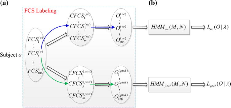
The method for classification of PTSD via HMMs. a The FCS sequence of a specific test subject is labeled based on the Euclidean distances between FCSs and CFCSs, resulting in two symbolic observation sequences. b The likelihood of the two observation sequences under their corresponding HMM are calculated, based on which the specific test subject is classified as a PTSD patient or a NC subject

To compute the likelihood of the FCS sequence of the test subject based on Eq. (7), we should generate the symbolic observation sequence corresponding to the FCS sequence first, i.e., FCS labeling. The FCS sequence is labeled based on the Euclidean distances between FCS and CFCSs. For example, if the distance between the i-th FCS of subject a, ${\mathit{FCS}}_{\mathit{i}}^{(\mathit{a})}$, and the j-th common FCS of NC, ${\mathit{CFCS}}_{\mathit{j}}^{(\mathit{nc})}$, is the smallest one among all the distances between ${\mathit{FCS}}_{\mathit{i}}^{(\mathit{a})}$ and ${\mathit{CFCS}}^{(\mathit{nc})}$, ${\mathit{FCS}}_{\mathit{i}}^{(\mathit{a})}$ is considered as another indirect measurement of the brain state which is indirectly measured by ${\mathit{CFCS}}_{\mathit{j}}^{(\mathit{nc})}$, and then labeled as the symbolic observation j. The same strategy is also performed between ${\mathit{FCS}}_{\mathit{i}}^{(\mathit{a})}$ and CFCS^(ptsd). After FCS labeling, two symbolic observation sequences corresponding to the FCS sequence, O^(nc) and O^(ptsd), can be obtained (Fig. 4a). Then, two likelihood, L_nc(O|λ) and L_ptsd(O|λ), which evaluate how well the HMMs for NC and PTSD can describe the FCS sequence, can be calculated by using the forward–backward algorithm (Fig. 4b) for classification purpose based on the following criteria. If L_nc (O|λ) < L_ptsd(O|λ), which means that HMM_ptsd(M, N) can better describe the FCS sequence of the test subject, the test subject is classified as a PTSD patient. On the contrary, if L_nc(O|λ) > L_ptsd(O|λ), the test subject is classified as a NC subject. The test subject cannot be classified when L_nc(O|λ) = L_ptsd(O|λ), which is very unlikely to happen actually but is possible theoretically. In our application, we had L_nc(O|λ) ≠ L_ptsd(O|λ) for all subjects.

Results

In this section, we designed and performed a series of experiments to evaluate the HMMs (“Hidden Markov Models Learnt for NC and PTSD” section) and apply them on a multimodal DTI/R-fMRI dataset of PTSD for classification purpose (“Classification of PTSD and NC via Multiple HMMs Using Majority Voting” section). Also, we examined the effect of the number of hidden and observed states in HMM (“Studies on the Effect of the Number of Hidden and Observed States in HMM” section) and the effect of the number of observation sequences for HMM learning (“Studies on the Effect of the Number of Observation Sequences for HMM Learning” section).

Hidden Markov Models Learnt for NC and PTSD

As described in “Functional Connectome State Construction” section, 51 observation sequences for NC and 44 observation sequences for PTSD were generated after FCS clustering, based on which we further learnt 121 HMMs for NC and another 121 HMMs for PTSD, with N and M both in the range of 15–25. The logarithm likelihood of the multiple observation sequences under each HMM was calculated and shown in Fig. 5. The logarithm likelihood of the multiple observation sequences of NC subjects reaches its local maximum at M of 16 and N of 21 (Fig. 5a), while the logarithm likelihood of the multiple observation sequences of PTSD patients reaches its local maximum at M of 16 and N of 24 (Fig. 5b).

Fig. 5.

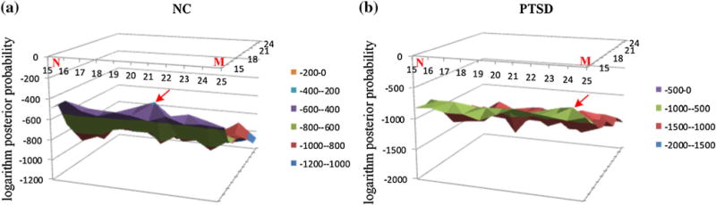
The logarithm likelihood of the multiple observation sequences of NC in a, and PTSD in b. The logarithm likelihood of the multiple observation sequences of NC reaches its local maximum at M of 16 and N of 21, where is highlighted by the red arrow in a, while the one of the multiple observation sequences of PTSD reaches its local maximum at M of 16 and N of 24, where is highlighted by the red arrow in b

Here, in order to quantitatively measure the transition patterns of the FBSs, we defined the number of the frequent states (NFS) and the degree of the transition patterns (DTP). For convenience, we use the compact notation QTP = (NFS, DTP) to indicate the quantitative property of the transition patterns (QTP). A state is considered as a frequent state if its occurrence in the transition patterns is greater than 1/8 of the total states. In this work, the value of 1/8 was determined experimentally. In the experiment, we tried the value of 1/n (n = 5, 6,…, 10). We empirically chose the number of 1/8 that achieved relatively significant result, in which there was at least one identified most frequent state in the transition patterns decoded from every learnt HMM. The DTP is just for counting the transitions, defined as:

$$\begin{array}{l}{\mathit{DTP}}^{(k)}={\displaystyle \sum _{i=1}^{T-1}{\mathit{DTP}}_{i,i+1};\mathit{\text{where}}{\mathit{DTP}}_{i,i+1}}\hfill \\ =\{\begin{array}{l}1,{\mathit{ifstate}}_i\ne {\mathit{state}}_{i+1}\hfill \\ 0,{\mathit{ifstate}}_i={\mathit{state}}_{i+1}\hfill \end{array}\hfill \end{array}$$ (8)

where state_i is the i_th state in the transition patterns and k denotes the subject index.

As shown in Fig. 5, HMM_nc (16, 21) and HMM_ptsd(16, 24) were the two best-matched HMMs, from which the underlying temporally dynamic transitions patterns of the FBSs were decoded by using the Viterbi algorithm, as shown in Fig. 6. The results in Fig. 6 demonstrate that the FBSs undergo remarkably temporally dynamic changes (Fig. 2f) in resting state, in agreement with previous studies (Li et al. 2013b; Chang and Glover 2010; Smith et al. 2012; Li et al. 2014; Gilbert and Sigman 2007; Majeed et al. 2011). Interestingly, the FBSs of NC subjects were mainly transiting amongst three frequent states (Fig. 6a), while the FBSs of PTSD patients were mainly stay in one state (Fig. 6b). The functional connectome patterns (Signature FCSs) characterizing those four most frequent FBSs were derived by averaging those FCSs that emitted the same underlying brain state and shown in Fig. 7. Our neuroscience interpretation is that NC brains tend to transit amongst two strongly-connected states and a relatively weakly connected state (Fig. 7a–c). In contrast, PTSD brains mainly stay in a strongly-connected state that involves the cingulate gyrus (Fig. 7d), which is believed to be involved in neural circuitries of PTSD (Francati et al. 2007). These results suggest that subjects wandered in and out of various cognitive states during the R-fMRI scan, without any control over the subject’s stimulus or environment. It is interesting that PTSD brains tend to stay in one state and seem to be unable to disengage from it. Moreover, the most frequent state in the transition patterns of PTSD is also an absorbing state in the Markov chain contained in HMM_ptsd(16, 24), which would be discussed in the following subsection.

Fig. 6.

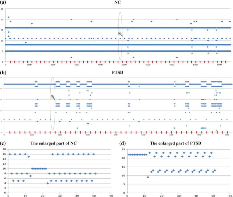
The joint multiple underlying temporally dynamic transition patterns of the FBSs for NC in a, and for PTSD in b, with the quantitative properties of (3, 181.4) and (1, 27.2). The temporally dynamic transition patterns in each area that split by the red line represented the dynamic transition patterns of an individual subject. For better illustration, we enlarged part of the transition patterns of NC in c, and PTSD in d

Fig. 7.

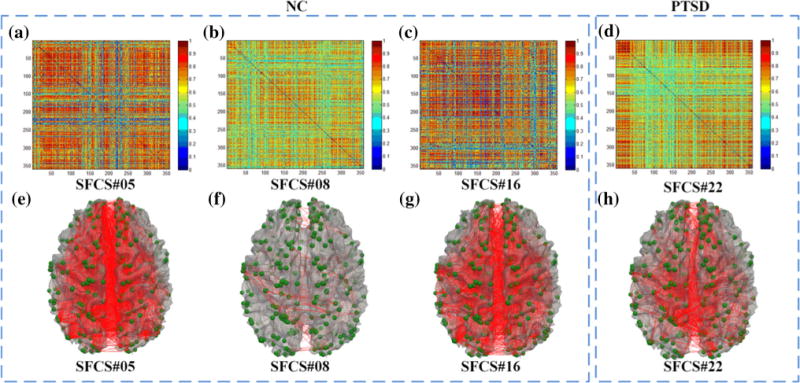
Visualization of the 358 × 358 functional connectome patterns of the 3 most frequent SFCSs of NC in a–c, and the most frequent SFCS of PTSD in d, and visualization of the functional connectome patterns of the above 4 most frequent SFCSs on cortical surfaces in e–h. DICCCOL ROIs are marked as green spheres on the cortical surface, and the functional connectivities between ROIs are shown as red edges connecting those spheres

Notably, the Markov chain contained in the HMM_nc(16, 21) is an ergodic, random walk, recurrent and regular one (Rabiner 1989; Stratonovich 1960). The state transition probabilities in HMM_nc(16, 21) converged after approximately 100 further prediction steps, and the equilibrium probabilities of the 21 underlying FBSs of NC subjects in HMM_nc(16, 21) were shown in Fig. 8. However, the state transition probabilities in HMM_ptsd(16, 24) converged much more slowly than the ones in HMM_nc(16, 21), which hadn’t converged after 15,000 prediction steps, as shown in Fig. 9. After convergence, there was an absorbing state (Fig. 7d, h), which suggested that the brains of PTSD patients tend to keep in that state after a long time R-fMRI scan. Due to the loud noise during the R-fMRI scan, it seemed impossible for subjects to become drowsy, even fall asleep. One possible interpretation is that PTSD patients become anxious or depression and tend to stay in that state, which reflects the previous hypothesis that brains with psychiatric conditions can be defined as the tendency to enter into, and inability to disengage from, a negative mood state (Holtzheimer and Mayberg 2011).

Fig. 8.

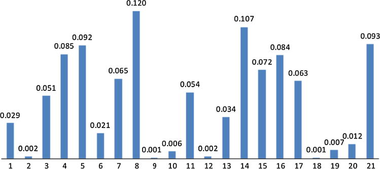
The equilibrium probabilities of the 21 underlying FBSs of NC subjects in HMM_nc(16, 21) after 100 further prediction steps

Fig. 9.

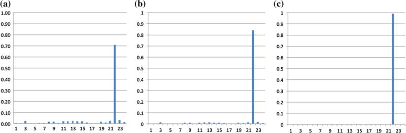
The probabilities of the 24 underlying FBSs of PTSD patients in HMM_ptsd(16, 24) after 10,000 prediction steps in a, 15,000 prediction steps in b, and 40,000 prediction steps in c

Classification of PTSD and NC via Multiple HMMs Using Majority Voting

First, to infer a robust and reproducible classification results, the commonly used n-fold cross validation strategy (n = 10) was adopted. The 44 PTSD patients and 51 NC subjects were equally divided into 10 portions (some portions may include one more patient or control). The cross-validation training set was subsequently constructed by sequentially combining nine portions, and the remaining was treated as the testing set. From “Hidden Markov Models Learnt for NC and PTSD” section, we have known that the likelihood of the observation sequences of NC and PTSD both reached their maxima with 16 observations. Therefore, we used the combinations of any two HMMs, one from NC and the other from PTSD, both with 16 observations and the number of hidden states in the range of 15–25, as classifiers. Thus, there were 121 classifiers for each fold. To get a better the classification accuracy, we combined these classifiers by using majority voting (Ruta and Gabrys 2005; Kittler et al. 1998) based on the premise that each classifier provides complementary information about the characteristics and difference of PTSD. A subject is considered as a PTSD patient when he/she is classified as a PTSD patient by more than half classifiers. On average, 37 PTSD patients out of 44, i.e., 84 %, and 44 NC subjects out of 51, i.e., 86 %, were successfully classified, as shown in Fig. 10. This classification accuracy is substantially better than the results reported in (Li et al. 2014) suggesting the superiority of the proposed HMMs and classification methods.

Fig. 10.

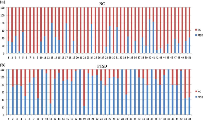
The classification result of multiple combinations of HMM_nc(16, N) and HMM_ptsd(16, N) using majority voting. The red bar indicates the votes that are classified as NC subject. The blue bar indicates the votes that are classified as PTSD patient. a 44 NC subjects won more than half votes that are classified as NC subjects. For example, the first subject won 89 votes that are classified as a NC subject and 32 votes that are classified as a PTSD patient. Through majority voting, the first subject is classified as a NC subject. b 37 PTSD patients won more than half votes that are classified as PTSD patients

Studies on the Effect of the Number of Hidden and Observed States in HMM

In this experiment, we chose two best-matched HMMs by the maximum likelihood of the multiple observation sequences, to decode the underlying dynamic transition patterns of the FBSs. In order to investigate the effect of the relative number of hidden states and observations during HMM learning, we also decoded the underlying dynamic transition patterns of the FBSs from other HMMs not only the two best-matched HMMs, and the quantitative properties of them for NC and PTSD were shown in Tables 1 and 2, respectively. The results suggested that all of the underlying transition patterns were similar, i.e., the underlying FBSs were mainly transiting amongst a few frequent states or mainly stayed in one state, and the brains of both NC and PTSD were under dynamic changes in resting state. Moreover, the PTSD brains mainly stayed in one state (Table 3), suggesting that PTSD could be characterized by the tendency to enter into, and more inability to disengage from, a negative mood state (Holtzheimer and Mayberg 2011).

Table 1.

The QTP of brain state transitions of NC with different values of N and M

N	15	16	17	18	19	20	21	22	23
M
15	(3, 181.4)	(2, 181.4)	(3, 181.3)	(1, 1.4)	(2, 180)	(1, 2.1)	(1, 4.8)	(2, 181.4)	(1, 3.4)
16	(2, 181.4)	(2, 181.4)	(2, 181.2)	(1, 21.7)	(2, 181.4)	(2, 181.4)	(3, 181.4)	(2, 181.4)	(1, 3.5)
17	(1, 3.3)	(1, 5)	(1, 4.7)	(1, 3.3)	(2, 178.3)	(1, 5.6)	(1, 6)	(2, 178.3)	(1, 3)
18	(2, 178.3)	(1, 3.7)	(1, 23.1)	(4, 178.3)	(1, 3.3)	(5, 176.6)	(1, 4.6)	(2, 178.2)	(1, 4.1)
19	(2, 178.1)	(1, 4.1)	(1, 7.5)	(3, 178.2)	(1, 2.4)	(2, 178.2)	(6, 178)	(3, 178.1)	(5, 178.2)
20	(2, 178.2)	(1, 2.3)	(1, 2.4)	(1, 10.4)	(2, 177.3)	(3, 178.2)	(2, 178.1)	(2, 178.2)	(5, 178.1)
21	(2, 178.2)	(2, 178)	(2, 178.2)	(1, 3.3)	(1, 4.1)	(2, 176.8)	(3, 178)	(2, 178.2)	(3, 177.4)
22	(2, 178.2)	(1, 2.4)	(4, 176.5)	(1, 4)	(1, 3.4)	(3, 178.1)	(1, 4.7)	(1, 6.1)	(1, 5.1)
23	(3, 178.1)	(1, 4.5)	(1, 3.9)	(1, 5)	(2, 177.9)	(1, 5.8)	(1, 4.3)	(3, 177.6)	(2, 178)
24	(4, 178.1)	(1, 3.4)	(3, 177.8)	(1, 3)	(1, 4.4)	(1, 3.3)	(2, 178.1)	(1, 3.3)	(1, 6.7)
25	(1, 4.2)	(3, 177.8)	(1, 3.5)	(2, 177.8)	(1, 2.6)	(1, 2.7)	(5, 177.8)	(5, 177.8)	(3, 177.5)

Table 2.

The QTP of brain state transitions of PTSD with different values of N and M

N	15	16	17	18	19	20	21	22	23
M
15	(3, 177.7)	(1, 3)	(1, 2.5)	(1, 2.2)	(1, 2.7)	(1, 1.9)	(3, 178.4)	(3, 177.8)	(1, 2.6)
16	(1, 3.9)	(1, 2.7)	(1, 3.4)	(4, 177.8)	(1, 9.9)	(2, 177.1)	(1, 3.5)	(1, 2.4)	(3, 177.8)
17	(2, 177.7)	(1, 3.2)	(3, 177.7)	(3, 177.6)	(1, 2.9)	(2, 177.7)	(3, 177.5)	(1, 2.7)	(2, 176.3)
18	(2, 173.9)	(2, 173.8)	(1, 5.9)	(2, 173.9)	(1, 4)	(3, 173.9)	(1, 6.8)	(5, 172.7)	(1, 4)
19	(2, 173.3)	(2, 173.9)	(1, 5.3)	(2, 173.7)	(1, 4.1)	(1, 6.5)	(1, 6.3)	(2, 173.7)	(3, 171.9)
20	(1, 4.1)	(1, 5.2)	(2, 173.8)	(2, 159.1)	(1, 3.8)	(3, 170)	(2, 173.2)	(3, 173.7)	(1, 2.7)
21	(1, 10)	(2, 173.1)	(2, 7.8)	(2, 173.9)	(1, 5.6)	(3, 173.7)	(1, 4.9)	(1, 3.8)	(3, 173.9)
22	(1, 5.3)	(3, 173.5)	(2, 177)	(4, 173.6)	(2, 173.6)	(1, 6.1)	(1, 5.2)	(1, 6)	(1, 6.1)
23	(2, 173.4)	(1, 4.5)	(1, 7.1)	(1, 2.4)	(3, 172.9)	(1, 4.2)	(1, 5.9)	(1, 4.2)	(1, 12.1)
24	(3, 173.5)	(2, 173.7)	(1, 6)	(1, 9.1)	(1, 4)	(1, 4.5)	(4, 173.7)	(1, 7.1)	(1, 3.7)
25	(2, 172.3)	(1, 5)	(1, 8.3)	(1, 4)	(1, 3.1)	(1, 8.1)	(1, 5.4)	(1, 5.7)	(1, 5.1)

Table 3.

The QTP of the best-matched HMMs and the classification results via them

Number		1	2	4	8	16	32	40
PTSD	(M,N)	(15, 22)	(16, 18)	(18, 24)	(25, 23)	(15, 20)	(15, 28)	(15, 25)
	QTP	(2, 0.5)	(2, 1.9)	(3, 69.8)	(2, 2.2)	(2, 4.9)	(2, 5.1)	(2, 6.8)
NC	(M,N)	(15, 19)	(24, 15)	(20, 17)	(15, 21)	(16, 20)	(15, 23)	(15, 16)
	QTP	(3, 109.4)	(4, 73.7)	(3, 74.1)	(3, 121.3)	(2, 7.4)	(2, 5.7)	(1, 5.9)
Classification		17/2a	10/9	2/8	9/8	19/12	15/29	24/29

^aThe entry of (17/2) means that 17 PTSD patients and 33 NC subjects are successfully classified

Studies on the Effect of the Number of Observation Sequences for HMM Learning

As discussed in “Functional Connectome State Construction” section, in order to cover larger brain state transition space and learn better matched HMMs, we used joint multiple observation sequences for HMM learning. In this experiment, we tried to learn HMMs by using different numbers of observation sequences and then to study the underlying dynamic transition patterns of the FBSs. Here, the number of hidden states, N, and the number of observations, M, were also in the range of 15–25, as used in “Hidden Markov Models Learnt for NC and PTSD” section. The evaluated numbers of observation sequences were 1, 2, 4, 8 16, 32 and 40. The best-matched HMMs learnt from a specific number of observation sequences were also determined by the maximum likelihood of the observation sequences. Then we calculated the quantitative properties of the underlying transition patterns decoded from the best-matched HMMs which were learnt from a given number of observation sequences, as shown in Table 3. Meanwhile, we also tried to classify PTSD patients and NC subjects via those HMMs based on the same methods in “HMM Modeling Based on Temporally Dynamic FCSs” section. The results of classification were also shown in Table 3. These results demonstrated that the more observation sequences we used for HMM learning, the more subjects can be classified successfully.

Discussion and Conclusion

In this work, we indirectly characterized the FBS by a large-scale functional connectivity matrix which was defined as the Pearson correlations between the windowed R-fMRI time series extracted from pairs of DICCCOL ROIs (Zhu et al. 2013). With the sliding time window, an FCS sequence of each brain was modeled and derived. After FCS clustering, we transformed the FCS sequence of each brain into a symbolic observation sequence, based on which we further learnt the HMMs to characterize the dynamic transition patterns of the FBSs.

Furthermore, the hidden parts of the HMMs were decoded and analyzed, and substantial and meaningful dynamic transition patterns of the FBSs of both NC and PTSD were discovered. The two best-matched HMMs were chosen by the maximum likelihood of the multiple observation sequences of NC and PTSD respectively, to decode the underlying temporally dynamic transition patterns of the FBSs. The results demonstrate that the FBSs undergo dynamic changes in resting state, in agreement with previous studies (Li et al. 2013b; Chang and Glover 2010; Smith et al. 2012; Li et al. 2014; Gilbert and Sigman 2007; Majeed et al. 2011). On average, 84 % of PTSD patients and 86 % of NC subjects were successfully classified via multiple HMMs using majority voting, which is substantially better than previously reported results (Li et al. 2014).

Additionally, the Markov chains contained in the two best-matched HMMs were analyzed and meaningful results of further predictions with the Markov chains were discovered. Further predictions with the best-matched HMM for PTSD revealed that there was an absorbing state in the Markov chain, which means the PTSD brains tend to keep in one state in the future. The FCSs and FCS transition modeling with HMMs in our work for PTSD are consistent with the brain state models in the PTSD study, which abstract brain functional connectivity as FBSs and represent mental status by a finite state transition space. In particular, our work presents a computation framework for modeling and representing the FBS dynamics via HMMs, providing direct support to the characterization and differentiation for psychiatric conditions.

In this study, we premise that FCS is an indirect measurement of FBS, and that different FCSs in different time windows and across different individuals may indirectly measure the same brain state. Therefore, we applied the hierarchical clustering to identify those FCSs which indirectly measure the same brain state, and then assigned them to the same symbolic observation state. We applied HMM learning to the symbolic observation sequences derived via the two-stage hierarchical clustering, rather than the FCS sequences directly. It should be mentioned that the reason why we adopted a two-stage hierarchical clustering strategy is due to limited commutating resource. For example, when we tried to apply the hierarchical clustering with the 9,486 × 9,486 distance matrix in matlab on a computer with 16 GB memory, it still raised the error of “out of memory”. Notably, the dynamic transition patterns of FBSs decoded from the two best-matched HMMs provided evidence to our premise that different FCS in different time windows and across different individuals indirectly measure the same brain state.

The work presented in this work can be further improved and enhanced in the future in the following aspects. First, in this work, we modeled the dynamic transition patterns of the FBSs via first-order HMMs, which are the simplest ones. Actually, the human brain is very complex, and there exist high-order dependencies between brain states, i.e., not only the current state determines how the brain transit to the next state, but also the previous states would affect the transition. By utilizing high-order HMMs in the future, we could be able to better model and characterize the temporally dynamic transitions of the brain states, reveal more phenomena and principles, and provide a more comprehensive way to understand the dynamics of the FBSs. Second, as the functional roles of DICCCOLs are discovered, we could analyze more biological meanings of those SFCSs. Third, besides PTSD, we plan to apply the similar HMMs to model and represent the functional brain dynamics in other scenarios such as during task performance and under natural stimulus, and in other brain conditions such as the psychiatric disorders of depression and bipolar disorders.

References

- Allen EA, Damaraju E, Plis SM, Erhardt EB, Eichele T, Calhoun VD. Tracking Whole-Brain Connectivity Dynamics in the Resting State. Cereb Cortex. 2012 doi: 10.1093/cercor/bhs352. [DOI] [PMC free article] [PubMed] [Google Scholar]
- Bassett DS, Wymbs NF, Porter MA, Mucha PJ, Carlson JM, Grafton ST. Dynamic reconfiguration of human brain networks during learning. Proc Natl Acad Sci USA. 2011;108(18):7641–7646. doi: 10.1073/pnas.1018985108. [DOI] [PMC free article] [PubMed] [Google Scholar]
- Binnewijzend MA, Schoonheim MM, Sanz-Arigita E, Wink AM, van der Flier WM, Tolboom N, Adriaanse SM, Damoiseaux JS, Scheltens P, van Berckel BN, Barkhof F. Resting-state fMRI changes in Alzheimer’s disease and mild cognitive impairment. Neurobiol Aging. 2012;33(9):2018–2028. doi: 10.1016/j.neurobiolaging.2011.07.003. [DOI] [PubMed] [Google Scholar]
- Biswal BB. Resting state fMRI: a personal history. Neuroimage. 2012;62(2):938–944. doi: 10.1016/j.neuroimage.2012.01.090. [DOI] [PMC free article] [PubMed] [Google Scholar]
- Biswal BB, Mennes M, Zuo XN, Gohel S, Kelly C, Smith SM, Beckmann CF, Adelstein JS, Buckner RL, Colcombe S, Dogonowski AM, Ernst M, Fair D, Hampson M, Hoptman MJ, Hyde JS, Kiviniemi VJ, Kotter R, Li SJ, Lin CP, Lowe MJ, Mackay C, Madden DJ, Madsen KH, Margulies DS, Mayberg HS, McMahon K, Monk CS, Mostofsky SH, Nagel BJ, Pekar JJ, Peltier SJ, Petersen SE, Riedl V, Rombouts SA, Rypma B, Schlaggar BL, Schmidt S, Seidler RD, Siegle GJ, Sorg C, Teng GJ, Veijola J, Villringer A, Walter M, Wang L, Weng XC, Whitfield-Gabrieli S, Williamson P, Windischberger C, Zang YF, Zhang HY, Castellanos FX, Milham MP. Toward discovery science of human brain function. Proc Natl Acad Sci USA. 2010;107(10):4734–4739. doi: 10.1073/pnas.0911855107. [DOI] [PMC free article] [PubMed] [Google Scholar]
- Chang C, Glover GH. Time-frequency dynamics of resting-state brain connectivity measured with fMRI. Neuroimage. 2010;50(1):81–98. doi: 10.1016/j.neuroimage.2009.12.011. [DOI] [PMC free article] [PubMed] [Google Scholar]
- Cordes D, Haughton V, Carew JD, Arfanakis K, Maravilla K. Hierarchical clustering to measure connectivity in fMRI resting-state data. Magn Reson Imaging. 2002;20(4):305–317. doi: 10.1016/s0730-725x(02)00503-9. [DOI] [PubMed] [Google Scholar]
- Dickerson BC, Sperling RA. Large-scale functional brain network abnormalities in Alzheimer’s disease: insights from functional neuroimaging. Behav Neurol. 2009;21(1):63–75. doi: 10.3233/BEN-2009-0227. [DOI] [PMC free article] [PubMed] [Google Scholar]
- Dijk KRAV, Hedden T, Venkataraman A, Evans KC, Lazar SW, Buckner RL. Intrinsic functional connectivity as a tool for human connectomics: theory, properties, and optimization. J Neurophysiol. 2010;103(1):297–321. doi: 10.1152/jn.00783.2009. [DOI] [PMC free article] [PubMed] [Google Scholar]
- Eavani H, Satterthwaite T, Gur R, Gur R, Davatzikos C. Unsupervised Learning of Functional Network Dynamics in Resting State fMRI. In: Gee J, Joshi S, Pohl K, Wells W, Zöllei L, editors. Information Processing in Medical Imaging, vol 7917, Lecture notes in computer science. Springer; Berlin Heidelberg: 2013. pp. 426–437. [DOI] [PMC free article] [PubMed] [Google Scholar]
- Ekman M, Derrfuss J, Tittgemeyer M, Fiebach CJ. Predicting errors from reconfiguration patterns in human brain networks. Proc Natl Acad Sci USA. 2012;109(41):16714–16719. doi: 10.1073/pnas.1207523109. [DOI] [PMC free article] [PubMed] [Google Scholar]
- Fox MD, Raichle ME. Spontaneous fluctuations in brain activity observed with functional magnetic resonance imaging. Nat Rev Neurosci. 2007;8(9):700–711. doi: 10.1038/nrn2201. [DOI] [PubMed] [Google Scholar]
- Francati V, Vermetten E, Bremner JD. Functional neuroimaging studies in posttraumatic stress disorder: review of current methods and findings. Depress Anxiety. 2007;24(3):202–218. doi: 10.1002/da.20208. [DOI] [PMC free article] [PubMed] [Google Scholar]
- Gilbert CD, Sigman M. Brain states: top-down influences in sensory processing. Neuron. 2007;54(5):677–696. doi: 10.1016/j.neuron.2007.05.019. [DOI] [PubMed] [Google Scholar]
- Hagmann P, Cammoun L, Gigandet X, Gerhard S, Ellen Grant P, Wedeen V, Meuli R, Thiran J-P, Honey CJ, Sporns O. MR connectomics: principles and challenges. J Neurosci Methods. 2010;194(1):34–45. doi: 10.1016/j.jneumeth.2010.01.014. [DOI] [PubMed] [Google Scholar]
- Holtzheimer PE, Mayberg HS. Stuck in a rut: rethinking depression and its treatment. Trends Neurosci. 2011;34(1):1–9. doi: 10.1016/j.tins.2010.10.004. [DOI] [PMC free article] [PubMed] [Google Scholar]
- Jain AK, Murty MN, Flynn PJ. Data Clustering: a Review. ACM Comput Surv. 1999;31(3):264–323. [Google Scholar]
- Jinli O, Li X, Peng W, Xiang L, Dajiang Z, Rongxin J, Yufeng W, Yaowu C, Jing Z, Tianming L. Modeling brain functional dynamics via hidden Markov models. Neural Engineering (NER), 2013 6th International IEEE/EMBS Conference on 6–8 Nov. 2013; pp. 569–572. [Google Scholar]
- Kennedy D. Making Connections in the Connectome Era. Neuroinformatics. 2010;8(2):61–62. doi: 10.1007/s12021-010-9070-1. [DOI] [PubMed] [Google Scholar]
- Kittler J, Hatef M, Duin RPW, Matas J. On combining classifiers. IEEE Trans Pattern Anal Mach Intell. 1998;20(3):226–239. [Google Scholar]
- Li K, Guo L, Nie J, Li G, Liu T. Review of methods for functional brain connectivity detection using fMRI. Comput Med Imaging Graph. 2009;33(2):131–139. doi: 10.1016/j.compmedimag.2008.10.011. [DOI] [PMC free article] [PubMed] [Google Scholar]
- Li K, Zhu D, Guo L, Li Z, Lynch ME, Coles C, Hu X, Liu T. Connectomics signatures of prenatal cocaine exposure affected adolescent brains. Hum Brain Mapp. 2013a;34(10):2494–2510. doi: 10.1002/hbm.22082. [DOI] [PMC free article] [PubMed] [Google Scholar]
- Li X, Lim C, Li K, Guo L, Liu T. Detecting brain state changes via fiber-centered functional connectivity analysis. Neuroinformatics. 2013b;11(2):193–210. doi: 10.1007/s12021-012-9157-y. [DOI] [PMC free article] [PubMed] [Google Scholar]
- Li X, Zhu D, Jiang X, Jin C, Zhang X, Guo L, Zhang J, Hu X, Li L, Liu T. Dynamic functional connectomics signatures for characterization and differentiation of PTSD patients. Hum Brain Mapp. 2014;35(4):1761–1778. doi: 10.1002/hbm.22290. [DOI] [PMC free article] [PubMed] [Google Scholar]
- Liang P, Wang Z, Yang Y, Jia X, Li K. Functional disconnection and compensation in mild cognitive impairment: evidence from DLPFC connectivity using resting-state fMRI. PLoS ONE. 2011;6(7):e22153. doi: 10.1371/journal.pone.0022153. [DOI] [PMC free article] [PubMed] [Google Scholar]
- Lynall M-E, Bassett DS, Kerwin R, McKenna PJ, Kitzbichler M, Muller U, Bullmore E. Functional connectivity and brain networks in schizophrenia. J Neurosci. 2010;30(28):9477–9487. doi: 10.1523/JNEUROSCI.0333-10.2010. [DOI] [PMC free article] [PubMed] [Google Scholar]
- Majeed W, Magnuson M, Hasenkamp W, Schwarb H, Schumacher EH, Barsalou L, Keilholz SD. Spatiotemporal dynamics of low frequency BOLD fluctuations in rats and humans. Neuroimage. 2011;54(2):1140–1150. doi: 10.1016/j.neuroimage.2010.08.030. [DOI] [PMC free article] [PubMed] [Google Scholar]
- Murtagh F. A survey of recent advances in hierarchical clustering algorithms. Comput J. 1983;26(4):354–359. [Google Scholar]
- Nianjun Liu, Davis Rial BC, Kootsookos PJ. Effect of initial HMM choices in multiple sequence training for gesture recognition. International Conference on Information Technology: Coding and Computing. 2004;1:608–613. [Google Scholar]
- Passingham RE, Stephan KE, Kotter R. The anatomical basis of functional localization in the cortex. Nat Rev Neurosci. 2002;3(8):606–616. doi: 10.1038/nrn893. [DOI] [PubMed] [Google Scholar]
- Rabiner LR. A tutorial on hidden Markov models and selected applications in speech recognition. Proc IEEE. 1989;77(2):257–286. [Google Scholar]
- Richiardi J, Eryilmaz H, Schwartz S, Vuilleumier P, Van De Ville D. Decoding brain states from fMRI connectivity graphs. Neuroimage. 2011;56(2):616–626. doi: 10.1016/j.neuroimage.2010.05.081. [DOI] [PubMed] [Google Scholar]
- Ruta D, Gabrys B. Classifier selection for majority voting. Information Fusion. 2005;6(1):63–81. [Google Scholar]
- Schwarz G. Estimating the dimension of a model. Ann Stat. 1978;6(2):461–464. [Google Scholar]
- Smith SM, Miller KL, Moeller S, Xu J, Auerbach EJ, Woolrich MW, Beckmann CF, Jenkinson M, Andersson J, Glasser MF, Van Essen DC, Feinberg DA, Yacoub ES, Ugurbil K. Temporally-independent functional modes of spontaneous brain activity. Proc Natl Acad Sci USA. 2012;109(8):3131–3136. doi: 10.1073/pnas.1121329109. [DOI] [PMC free article] [PubMed] [Google Scholar]
- Sporns O, Tononi G, Kötter R. The human connectome: a structural description of the human brain. PLoS Comput Biol. 2005;1(4):e42. doi: 10.1371/journal.pcbi.0010042. [DOI] [PMC free article] [PubMed] [Google Scholar]
- Stebbins GT, Murphy CM. Diffusion tensor imaging in Alzheimer’s disease and mild cognitive impairment. Behav Neurol. 2009;21(1):39–49. doi: 10.3233/BEN-2009-0234. [DOI] [PMC free article] [PubMed] [Google Scholar]
- Stratonovich RL. Conditional Markov Processes. Theory Prob Appl. 1960;5(2):156–178. [Google Scholar]
- Williams R. The human connectome: just another ‘ome? Lancet Neurol. 2010;9(3):238–239. doi: 10.1016/S1474-4422(10)70046-6. [DOI] [PubMed] [Google Scholar]
- Zhang X, Guo L, Li X, Zhang T, Zhu D, Li K, Chen H, Lv J, Jin C, Zhao Q, Li L, Liu T. Characterization of task-free and task-performance brain states via functional connectome patterns. Med Image Anal. 2013;17(8):1106–1122. doi: 10.1016/j.media.2013.07.003. [DOI] [PMC free article] [PubMed] [Google Scholar]
- Zhu D, Li K, Guo L, Jiang X, Zhang T, Zhang D, Chen H, Deng F, Faraco C, Jin C, Wee C-Y, Yuan Y, Lv P, Yin Y, Hu X, Duan L, Hu X, Han J, Wang L, Shen D, Miller LS, Li L, Liu T. DICCCOL: dense individualized and common connectivity-based cortical landmarks. Cereb Cortex. 2013;23(4):786–800. doi: 10.1093/cercor/bhs072. [DOI] [PMC free article] [PubMed] [Google Scholar]