A Novel Cortical Thickness Estimation Method based on Volumetric Laplace-Beltrami Operator and Heat Kernel

Abstract

Cortical thickness estimation in magnetic resonance imaging (MRI) is an important technique for research on brain development and neurodegenerative diseases. This paper presents a heat kernel based cortical thickness estimation algorithm, which is driven by the graph spectrum and the heat kernel theory, to capture the grey matter geometry information from the in vivo brain magnetic resonance (MR) images. First, we construct a tetrahedral mesh that matches the MR images and reflects the inherent geometric characteristics. Second, the harmonic field is computed by the volumetric Laplace-Beltrami operator and the direction of the steamline is obtained by tracing the maximum heat transfer probability based on the heat kernel diffusion. Thereby we can calculate the cortical thickness information between the point on the pial and white matter surfaces. The new method relies on intrinsic brain geometry structure and the computation is robust and accurate. To validate our algorithm, we apply it to study the thickness differences associated with Alzheimer’s disease (AD) and mild cognitive impairment (MCI) on the Alzheimer’s Disease Neuroimaging Initiative (ADNI) dataset. Our preliminary experimental results on 151 subjects (51 AD, 45 MCI, 55 controls) show that the new algorithm may successfully detect statistically significant difference among patients of AD, MCI and healthy control subjects. Our computational framework is efficient and very general. It has the potential to be used for thickness estimation on any biological structures with clearly defined inner and outer surfaces.

1. Introduction

Alzheimer’s disease (AD) is the most common form of cognitive disability in older people. With the population living longer than ever before, AD is now a major public health concern with the number of affected patients expected to triple, reaching 13.5 million by the year 2050 in the U.S. alone (Alzheimer’s Association, 2012). It is commonly agreed that an effective presymptomatic diagnosis and treatment of AD could have enormous public health benefits (Sperling et al., 2011). Brain imaging has the potential to provide valid diagnostic biomarkers of AD risk factors and preclinical stage AD (Caselli and Reiman, 2013; Langbaum et al., 2013). Despite major advances in brain imaging used to track symptomatic patients (as reviewed in Chung, 2012), there is still a lack of sensitive, reliable, and accessible brain imaging algorithms capable of characterizing abnormal degrees of age-related cerebral atrophy, as well as accelerated rates of atrophy progression in preclinical individuals at high risk for AD for whom early intervention is most needed.

In AD research, structural magnetic resonance imaging (MRI) based measures of atrophy in several structural measures, including whole-brain (Fox et al., 1999; Chen et al., 2007; Stonnington et al., 2010; Thompson et al., 2003), entorhinal cortex (Cardenas et al., 2011), hippocampus (den Heijer et al., 2010; Jack et al., 2003; Reiman et al., 1998; Thompson et al., 2004; Wolz et al, 2010; Wang et al., 2011; Shi et al., 2013a), and temporal lobe volumes (Hua et al., 2010), as well as ventricular enlargement (Jack et al., 2003; Wang et al., 2011) correlate closely with changes in cognitive performance, supporting their validity as markers of disease progression (as reviewed in Braskie and Thompson, 2013). As one of major AD symptoms on clinical anatomy, the partial atrophy in the cerebral cortex of the patients is a biomarker of AD progress (Braak and Braak, 1991). To check and monitor the cortical atrophy, a number of research has been focused on an accurate estimation of cortical thickness (e.g. MacDonald et al., 2000; Fischl and Dale, 2000; Jones et al., 2000; Miller et al, 2000; Kabani et al, 2001; Chung et al., 2005; Kochunov et al., 2012). However, the MRI imaging measurement of cortical thickness, e.g. medial temporal atrophy, is still not sufficiently accurate on its own to serve as an absolute diagnostic criterion for the clinical diagnosis of AD at the mild cognitive impairment (MCI) stage (Frisoni et al., 2010).

According to geometric properties of the measurement tools, the cortical thickness estimation methods can be broadly divided into two categories: based on either surface or voxel characteristics (as reviewed in Clarkson et al., 2011). The measurement methods based on the surface features are aimed to establish triangular mesh models in accordance with the topological properties of the inner and outer surfaces, and then use the deformable evolution model to couple the two opposing surfaces. The thickness is defined as the value of the level set propagation distance between the two surfaces. This measurement accuracy can reach the sub-pixel level but requires constantly correcting the weights of various evolutionary parameters to ensure the mesh regularity. Sometimes the model can not work in the highly folding regions such as the sulci. Various approaches were proposed to address this problem and increase the thickness estimation accuracy in the high curvature areas. For example, Mak-Fan and colleagues modeled the sulci regional by adding the cortex thickness constraints (Mak-Fan et al., 2012). Fischl and Dale (2000) proposed to model the middle part of the sulci by imposing the self-intersection constraints. Overall, although better measurement results are achieved, the computation cost is generally high (Dahnke et al., 2013). In contrast, the voxel-based method is the measurement on a three-dimensional cubic voxel grid. The voxel-based measurement acquires the cortical thickness information by solving partial differential equations in the potential field, for example, Jones et al. (2000) first used the Laplace equation to characterize the layered structure of the volume between the inner and outer surfaces and obtained the stream line. This method is known as the Lagrangian method. Hyde et al. (2012) proposed the Euler method by solving the one-order linear partial differential equations for thickness calculation which can improve the computation efficiency. The advantages of such an approach include: (1). there is no correction of the mesh topology regularity, so the calculation is simple (Cardoso et al., 2011; Das et al., 2009); (2). the computational model is rigorous and stable. The main disadvantage of the voxel-based estimation method is the computational inaccuracy on the discrete grid. The limited grid resolution affects the accuracy of the thickness measurement (Das et al., 2009). This problem is alleviated only recently. For example, Jones and Chapman (2012) used the boundary topology to initialize a sub-voxel resolution surface and correct the direction of the stream line. This method can increase the measurement accuracy.

From the above discussion, in order to improve the computational efficiency and the degree of automation, one may expect the choice of voxel-based measurement algorithm is more feasible. However, we should overcome the defect of the limited grid resolution which can not precisely characterize the curved cortical surfaces from MR images. This point will be discussed in Discussion Section. A desired 3D model should achieve a good fitting for the cerebral cortex morphology and facilitate an effective computation on the sub-voxel resolution. In this paper, we propose to use tetrahedral mesh (Cassidy et al., 2013) to model the volume between inner and outer cortical surface. For thickness estimation, we adopt the tetrahedral mesh based Laplace-Beltrami operator proposed in our prior work (Wang et al., 2004a), which has been frequently adopted by volumetric shape analysis research (Wang et al, 2004b; Li et al, 2007; Tan et al., 2010; Pai et al, 2011; Li et al., 2010; Paillé and Poulin, 2012; Wang et al, 2012a; Xu et al., 2013a; Li et al., 2013). Generally speaking, the tetrahedral mesh access is time consuming. We extend the half-edge data structure (Mäntylä, 1988) to a half-face data structure for an efficient geometric processing.

Based on spectral analysis theory, we further propose to compute a heat kernel (Hsu, 2002) based method to trace the streamlines between inner and outer cortical surfaces and estimate the cortical thickness by computing the streamline lengths. Mathematically speaking, diffusion kernels (Coifman et al., 2005b) express the transition probability by random walk of t steps, t ≥ 0. It allows for defining a scale space of kernels with the scale parameter t. Such heat kernel-based spectral analysis induces a robust and multi-scale metric to compare different shapes and has strong theoretical guarantees. In recent years, surface based heat kernel methods have been widely used in computer vision and medical image analysis (Chung et al., 2005; Sun et al, 2009; Chung, 2012; Joshi et al., 2012; Lombaert et al, 2012; Litman and Bronstein, 2014), such as functional and structural map smoothing (Qiu et al., 2006a,b; Shi et al., 2010, 2013b), classification (Bronstein and Bronstein, 2011), and registration (Sharma et al., 2012). However, 3D heat kernel methods are still rare in medical image analysis field. Some pioneering work (Raviv et al., 2010; Rustamov, 2011) used regular grids to compute the heat kernel and their work usually suffered numerical inaccuracies along the surface boundaries. Based on the volumetric Laplace-Beltrami operator, our heat kernel computation is more accurate and the estimated cortical thickness is well-defined, and should reflect the intrinsic 3D geometrical structure better than thickness derived from a simple harmonic field (Jones et al., 2000), and hence facilitate consistent cross-subject comparisons.

In our experiments, our pipeline is applied on MR images from Alzheimer’s Disease Neuroimaging Initiative (Mueller et al., 2005; Jack et al., 2008, ADNI). Our data set consists of: 51 patients of Alzheimer’s disease (AD), 45 patients of mild cognitive impairment (MCI) and 55 healthy controls. We use FreeSurfer software (Fischl et al., 1999a) for preprocessing. We use Student’s t test and False Discovery Rate (FDR) (Benjamini and Hochberg, 1995) for performance evaluation. We set out to test whether our proposed method provides a computationally efficient and statistically powerful cortical thickness solution.

Fig. 1 summarizes our overall sequence of steps used to compute cortical thickness. First, from MR images, we used FreeSurfer to segment and build white matter and pial cortical surfaces (the first and second row). We model the inner volume with a tetrahedral mesh with a triangle surface as it boundary (the third row). Then we apply volumetric Laplace-Beltrami operator to compute the harmonic field and build isothermal surfaces on the obtained harmonic field. Between neighboring isothermal surfaces, we compute heat kernel and estimate the streamline by tracing the maximal heat transition probability. The thickness is then measured by the lengths of the streamlines between white matter and pial surfaces (the fourth row). Last, Student’s t test is applied to identify regions with significant differences between any two of three groups and false discovery rate (FDR) (Nichols and Hayasaka, 2003) is used to assign global q-values (the fifth row), i.e., all group difference p-maps were corrected for multiple comparisons using the widely-used FDR method. For example, the FDR method decides whether a threshold can be assigned to the statistical map that keeps the expected false discovery rate below 5% (i.e., no more than 5% of the voxels are false positive findings).

Figure 1.

Algorithm pipeline illustrated by the intermediate results.

2. Methods and Materials

2.1. Tetrahedral Mesh Generation Module

It is worth noticing that the tetrahedral mesh quality will affect the accuracy of solving the partial differential equations. For example, too small dihedral angles will lead to ill-posed stiffness matrix in the finite element method and too large dihedral angles will lead to the interpolation and discretization errors. The common tetrahedron generation method is to revise the tetrahedrons through the iterative processing. One class of methods are to divide the voxels of the MRI to tetrahedrons according to the generation quality (Liu and Xing, 2013). But it usually results in the loss of the original image information because of the lack of the boundary restriction conditions. Another class of methods intends to comply with the precise topology structure of the original image by adaptively adjusting the size of the tetrahedrons (Lederman et al., 2010), which constantly use the external force to pull the tetrahedral vertices to the boundary of the MRI. However, it neglects the quality of each tetrahedron.

Although there is a rich literature on the tetrahedral mesh generation for medical imaging research (e.g. Zhang et al., 2005; Lederman et al., 2011; CGAL Editorial Board, 2013; Min, 2013; Fang and Boas, 2009; Si, 2010; Kremer, 2011), it is still challenging to model the highly convoluted cortical structure. In our prior work (Wang et al., 2004a), we proposed a sphere carving method to use tetrahedral mesh to model cortical structure while enforcing a correct topology on the obtained boundary surfaces. In our current approach, we build a robust tetrahedral mesh generation module by incorporating a few existing free mesh processing utilities (Min, 2013; Nooruddin and Turk, 2003; CGAL Editorial Board, 2013; Lederman et al., 2011). Our work keeps a balance between surface fitness and tetrahedral mesh quality by carefully tuning their parameters to model cortical structure. The pipeline of our tetrahedral mesh generation algorithm for the MR images is shown in Fig. 2.

Figure 2.

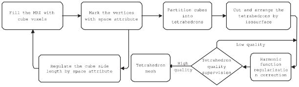
Tetrahedral mesh generation work flow.

First we fill the MRI space with the cubic background voxels with binvox software (Min, 2013; Nooruddin and Turk, 2003). The space attribute of each voxel vertex is determined by the point-to-boundary distance function ϕ(x). ϕ(x) is calculated using the fast marching method (Sethian, 1996). Based on ϕ(x) values, we can adaptively adjust the filled cubic length by calculating the vertex coordinates(x or y) difference of the adjacent boundary surface with the same z coordinate. Secondly, the cubic voxel containing the boundary surface and the internal voxel are split into the tetrahedrons using smoothing modules in software package CGAL (CGAL Editorial Board, 2013).

The obtained tetrahedral mesh needs to be corrected to improve the quality and the smoothness owing to the cutting and organization operations. We call the process as the regularization for the boundary smoothness and tetrahedron quality improvement (CGAL Editorial Board, 2013; Lederman et al., 2011). We adopted CGAL (CGAL Editorial Board, 2013) for this purpose. This process is based on harmonic function minimization (CGAL Editorial Board, 2013; Lederman et al., 2011) which regularizes the mesh generation by minimizing an energy term which consists of elastic term, smoothness term, fidelity term on the shape regularity (Lederman et al., 2011). Fig. 3 shows the two examples of generated tetrahedral meshes with the different resolutions and their tetrahedral element qualities. In the upper row, the figures from the left to the right are the generated tetrahedral mesh (154,908 tetrahedrons) based on our method, the cross-section cut through the mesh according to y-axis, the dihedral angle histograms and the tetrahedral element quality coefficients respectively. The tetrahedral element quality coefficients will be discussed in the Discussion Section. The bottom row indicates the same contents as the upper row except the number of the tetrahedron elements is 382,071. The numbers within the square brackets in the two right columns represent the value ranges of the dihedral angle and the quality coefficients. From the result, we find that our approach can produce the better tetrahedron element quality under the premise of maintaining the original shape of the object.

Figure 3.

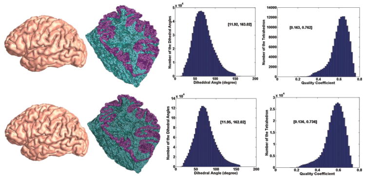
Two examples of generated tetrahedral meshes with the different resolutions and their tetrahedral element qualities.

2.2. Half-Face Data Structure for Representing Tetrahedral Meshes

To efficiently access the generated tetrahedral mesh for cortical thickness estimation, we extended half-edge data structure (Mäntylä, 1988) to half-face data structure (e.g. Kremer, 2011). A half-edge data structure is an edge-centered data structure capable of maintaining incidence information of vertices, edges and faces for any orientable two-dimensional surfaces embedded in arbitrary dimension. Each edge is decomposed into two half-edges with opposite directions. Centered in half-edges, pointers are added to point to other connected instances, such as vertices, faces and edges. An overview and comparison of these different data structures together with a thorough description of the implementation details can be found in Kettner (1999).

Fig. 4(a) illustrates some key concepts in half-edge data structure. It is widely used in computer graphics and geometric modeling research. We extended it to model tetrahedral mesh structure. In our approach, we added a half-face layer over the half-edge layer (Fig. 4(b)). Similar to half-edge structure, each face is decomposed into two half-faces with opposite directions and appropriate pointers are added to connect tetrahedrons, faces, edges and vertices. Such a data structure, with a cost of additional storage space for added pointers, helps us improve the computational efficiency dramatically. For example, if we want to access an adjacent tetrahedron, the time complexity for a brute force is about O(N), where N is the number of tetrahedrons, while the time complexity is just O(1) with our proposed half-face data structure (Xu, 2013).

Figure 4.

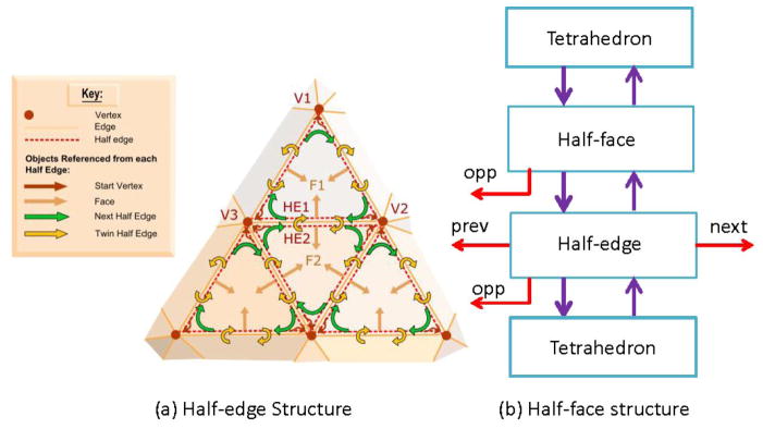
Illustration of half-edge structure for surface representation (a) and the proposed half-face structure for tetrahedron representation (b). (a) was obtained from (MakeHuman Project Team, 2013).

2.3. Thickness Measurement Algorithm based on the Heat Kernel Diffusion

2.3.1. Theoretical Background

The heat kernel diffusion on differentiable manifold M with Riemannian metric is governed by the heat equation:

$${\mathrm{\Delta }}_{M}f(x,t)=\frac{\partial f(x,t)}{\partial t}$$ (1)

where f(x, t) is the heat distribution of the volume at the given time. We know that the heat diffusion process can be represented by its time dependent and its spatially dependent parts.

$$f(x,t)=F(x)T(t)$$ (2)

Eq. 2 is substituted to Eq. 1, we can get the Helmholtz equation to describe the heat vibration modes in the spatial domain.

$$\mathrm{\Delta }F(x)=-\lambda F(x)$$ (3)

Eq. 3 can be treated as the Laplacian eigenvalue problem with infinite number of eigenvalue λ_i and eigenfunction F_i pairs. The solution of equation above can be interpreted to the superposition of the harmonic functions in the given spatial position and time. Given an initial heat distribution F : M → , let H_t(F) denotes the heat distribution at time t, and lim_t→0 H_t(F) = F. H(t) is called the heat operator. Both Δ_K and H_t share the same eigenfunctions, and if λ_i is an eigenvalue of Δ_M, then e^−λ_it is an eigenvalue of H_t corresponding to the same eigenfunction.

For any compact Riemannian manifold, there exists a function l_t(x, y) : ℝ⁺ × M×M → ℝ, satisfy the formula

$$H_{t}F(x)={\int }_M{l}_t(x,y)F(y)dy$$ (4)

where dy is the volume form at y ∈ M. The minimum function l_t(x, y) that satisfies Eq. 4 is called the heat kernel (Coifman et al., 2005b), and can be considered as the amount of heat that is transferred from x to y in time t given a unit heat source at x. In other words, l_t(x,·) = H_t(δ_x) where δ_x is the Direc delta function at x : δ_x(z) = 0 for any z ≠ x and ∫_M δ_x(z) = 1.

According to the theory of the spectral analysis, for compact M, the heat kernel has the following eigen-decomposition expression:

$$l_t(x,y)=\sum _{i=0}^{\infty }{e}^{-{\lambda }_{i}t}{\varphi }_i(x){\varphi }_i(y)$$ (5)

Where λ_i and ϕ_i are the i^th eigenvalue and eigenfunction of the Laplace-Beltrami operator, respectively. The heat kernel l_t(x, y) can be interpreted as the transition density function of the Brownian motion on the manifold (Sun et al., 2009). It has significant applications in computer vision and machine learning fields (Chung et al., 2005; Coifman et al., 2005a; Bronstein and Bronstein, 2011; Lombaert et al., 2012).

2.3.2. Discrete Harmonic Energy

Suppose M is a simplicial complex, and g : |M| → ℝ³ a function that embeds |M| in ℝ³, then (M, g) is called a mesh. For a 3-simplex, it is a tetrahedral mesh, Te, and for a 2-simplex, it is a triangular mesh, Tr. Clearly, the boundary of a tetrahedral mesh is a triangular mesh, Tr = ∂Te. All piecewise linear functions defined on M form a linear space, denoted by C^PL(M). Suppose a set of string constants k(u, v) are assigned, then the inner product on C^PL(M) is defined as the quadratic form:

$$<f,g>=\frac{1}{2}\sum _{\{u,v\}\in M}k(u,v)(f(u)-f(v))(g(u)-g(v))$$ (6)

The energy is defined as the norm on C^PL(M),

Definition 1 (String Energy)

Suppose f ∈ C^PL(M), the string energy is defined as:

$$E(f)=<f,f>=\sum _{\{u,v\}\in K}k(u,v){\Vert f(u)-f(v)\Vert }^2$$ (7)

By changing the string constants k(u, v) in the energy formula, we can define different string energies.

Definition 2 (Discrete Harmonic Energy)

(Wang et at., 2004a)] Suppose that edge {u, v}is shared by n tetrahedrons. In each tetrahedron, there is an edge which does not intersect with {u, v}, e.g. edge [v₁, v₄] and [v₂, v₃] pair in Fig. 5. By convention, we say that this edge is against {u, v} in this tetrahedron. Thus edge {u, v} is against a total of n edges in these n tetrahedrons. We denote their edge lengths as l_i, i = 1, …, n. Similarly, there is a dihedral angle which is associated with each edge, e.g. θ₂₃ is associated with edge [v₂, v₃] in Fig. 5. They can be denoted as, θ_i = 1, …, n. The dihedral angle θ is also said to be against edge [u, v]. So edge {u, v} is against a total of n dihedral angles, θ_i, i = 1, …, n, in these n tetrahedrons. Define the parameters

Figure 5.

Illustration of a tetrahedron. By convention, we say that the edge [v₁, v₄] is against [v₂, v₃] and the dihedral angle, θ_23, in this tetrahedron. l₂₃ is the length of edge [v₂, v₃]. This relationship is used to define volumetric Laplace-Beltrami operator.

$$k_{u,v}=\frac{1}{12}\sum _{i=1}^n{l}_{i}cot({\theta }_i)$$ (8)

where l_i, i = 1, …, n, are the lengths of the edges to which edge {u, v} is against in the domain manifold M. Eqn. 7 with the k_u,v is defined as the discrete harmonic energy.

Furthermore, our prior work (Xu, 2013) also proved that the discrete harmonic energy is consistent with the traditional harmonic energy.

2.3.3. Volumetric Laplace-Beltrami Operator

In this step, we use the discrete harmonic energy to compute the temperature distribution under the condition of the thermal equilibrium. The problem is to solve the Laplace equation Δt = 0 in the cortex region Ω subject to Dirichlet boundary conditions on ∂Ω, i.e., the temperature of the outer cortical surface equals to 1 and the temperature of the inner cortical surface equal to 0.

First we define the tetrahedral mesh of the cortex as the finite solution space and the interior nodes and boundary nodes. Owing to the shape regularity of the generated tetrahedral mesh, we can ensure the correctness in the finite element computation. Then we compute the local stiffness matrix S according to the specific tetrahedron mesh:

$$S_{i,j}=\{\begin{array}{ll}{k}_{i,j}& [i,j]\in \mathit{edge}\\ 0& [i,j]\notin \mathit{edge}\end{array}$$ (9)

Where k_i,j is defined in Definition 2. Clearly, S is a sparse matrix. Secondly, add the contribution of the local stiffness matrix to global stiffness matrix and construct the discrete Laplace-Beltrami operator under the Dirichlet boundary condition. The volumetric Laplace-Beltrami operator L_p is defined with the form:

$$L_p=D-S$$ (10)

where D, the degree matrix, is a diagnal matrix defined as D_ii = Σ_jS_ij.

Therefore, one may use the following equation to compute the temperature of the interior vertices.

$$L_p{t}_i=t_b$$ (11)

where t_i is a n × 1 vector (n is the number of the interior vertices in the tetrahedral mesh), and t_b is a m × 1 vector (m is the number of the boundary vertices in the tetrahedral mesh). As a result, we can translate solving the Laplace equation problem into solving a sparse linear system problem. The solution, also called as harmonic field, is also the internal temperature distribution inside the cortex.

Compared with other rasterization-based Laplace-Beltrami operator computation methods (e.g. Raviv et al., 2010; Rustamov, 2011), owing to the multi-resolution nature of the tetrahedral mesh, our method may capture and quantify local volumetric geometric structure more accurately. Similarly to some prior work (e.g. Tsukerman, 1998), we can rigorously prove that the proposed discrete harmonic energy will converge to the continuous harmonic energy with the increased tetrahedral mesh resolution.

2.3.4. Cortical Thickness Estimation with Heat Kernel

After we compute the harmonic field, we can construct the isothermal surfaces. With the defined volumetric Laplace-Beltrami operator, it is straightforward to compute the heat kernel (Eqn. 5) and apply it to estimate the cortical thickness. Specifically, the l_t(x, y) of the specific point x on an isothermal surface m to a different point y on the next isothermal surface m′ represents the different heat transition probability. The connection direction of the x and y according to the maximum transition probability is the direction of the temperature gradient. And then y as a starting point, we will continue to search for the next point y′ in the next isothermal surface n whose l_t(y, y′) is the maximum among the all l_t(y, ·) by repeating this process. So a streamline of the cortex will be obtained by finding out the maximum heat transition probability between the isothermal surfaces. Similar to prior work (Jones et al., 2000), the cortical thickness is estimated as the total length of the streamline.

However, our work is different from prior work (Jones et al., 2000) when tracing the streamline, where the normals of isothermal surfaces are always used to travel to neighboring isothermal surface. Our motivation is illustrated in Fig. 6. The heat diffusion is illustrated with spectrum (Fig. 6(a)) and the diffusion distance is illustrated in Fig. 6(b). Because it models heat diffusion more precisely, the heat kernel approach considers more intrinsic geometry structures and hence may produce more robust and accurate cortical thickness estimations.

Figure 6.

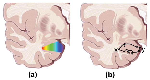
Illustration of heat diffusion on cortical structure. Two boundaries are examples of pial and white matter surfaces. (a) Heat diffusion illustration with spectrum; (b) diffusion distance illustrated as random walk. Our heat kernel method may be able to capture the subtle difference determined by the intrinsic geometry structures because it estimates the heat transition probability on every intermediate point such that it may capture more regional information than other harmonic function methods (e.g. Jones et al., 2000).

2.4. Experiments and Validation

2.4.1. Subjects

Data used in the preparation of this article were obtained from the Alzheimers Disease Neuroimaging Initiative (ADNI) database (adni.loni.usc.edu). The ADNI was launched in 2003 by the National Institute on Aging (NIA), the National Institute of Biomedical Imaging and Bioengineering (NIBIB), the Food and Drug Administration (FDA), private pharmaceutical companies and non-profit organizations, as a $60 million, 5-year public-private partnership. The primary goal of ADNI has been to test whether serial magnetic resonance imaging (MRI), positron emission tomography (PET), other biological markers, and clinical and neuropsychological assessment can be combined to measure the progression of mild cognitive impairment (MCI) and early Alzheimers disease (AD). Determination of sensitive and specific markers of very early AD progression is intended to aid researchers and clinicians to develop new treatments and monitor their effectiveness, as well as lessen the time and cost of clinical trials. The Principal Investigator of this initiative is Michael W. Weiner, MD, VA Medical Center and University of California San Francisco. ADNI is the result of efforts of many co-investigators from a broad range of academic institutions and private corporations, and subjects have been recruited from over 50 sites across the U.S. and Canada. The initial goal of ADNI was to recruit 800 subjects but ADNI has been followed by ADNI-GO and ADNI-2. To date these three protocols have recruited over 1500 adults, ages 55 to 90, to participate in the research, consisting of cognitively normal older individuals, people with early or late MCI, and people with early AD. The follow up duration of each group is specified in the protocols for ADNI-1, ADNI-2 and ADNI-GO. Subjects originally recruited for ADNI-1 and ADNI-GO had the option to be followed in ADNI-2. For up-to-date information, see www.adni-info.org.

At the time of downloading (09/2010), there were 843 subjects in the ADNI baseline dataset. All subjects underwent thorough clinical and cognitive assessment at the time of acquisition, including the Mini-Mental State Examination (MMSE) score (Folstein et al., 1975), Clinical Dementia Rating (CDR) (Berg, 1988), and Delayed Logical Memory Test (Wechsler, 1987).

In this study, the T1-weighted images from 151 subjects were used. The structural MRI images were from the ADNI baseline dataset (Mueller et al., 2005; Jack et al., 2008). We used FreeSurfer’s automated processing pipeline (Dale et al., 1999; Fischl et al., 1999a) for automatic skull stripping, tissue classification, surface extraction, and cortical and subcortical parcellations. It also calculates volumes of individual grey matter parcellations in mm³ and surface area in mm², provides surface and volume statistics for about 34 different cortical structures, and computes geometric characteristics such as curvature, curvedness, local foldedness for each of the parcellations (Desikan et al., 2006). In our experiments, our data set consists of 51 patients of Alzhermer’s disease (AD), 45 patients of mild cognitive impairment (MCI) and 55 healthy controls. And the demographic information of studied subjects in ADNI baseline dataset is in Table 1 Here MMSE is short for mini-mental state examination. It is a measurement of one’s IQ. Full score is 30, lower means more demented. So AD patients generally have low score.

Table 1.

Demographic information of studied subjects in ADNI baseline dataset.

	Gender(M/F)	Education	Age	MMSE at Baseline
AD	23/28	14.42 ± 2.23	76.67 ± 6.01	23.44 ± 2.21
MCI	23/22	16.05 ± 2.61	76.50 ± 6.51	27.25 ± 1.51
CTL	21/34	16.07 ± 2.39	76.31 ± 4.27	29.23 ± 0.85

2.4.2. Experiments

In our experiments, we first applied the new method on some synthetic volumetric data (Sec. 3.1) to evaluate the correctness of our algorithms. We built tetrahedral meshes on the MRI data of 151 ADNI subjects. As a proof-of-the-concept work, the thickness measurement based on heat kernel is applied on the left hemispheres. We applied the Student’s t test on sets of thickness values measured on corresponding surface points to study the statistical group difference. Given each matching surface point, we measure the difference between the mean thickness of three different groups (AD vs. control, MCI vs. control and AD vs. MCI) by

$$t=\frac{\overline{U}-\overline{V}}{\sqrt{\frac{2}{n}}{S}_{UV}}$$ (12)

where Ū and V̄ are the thickness means of the two groups and S_UV is the standard deviation. The denominator of t is the standard error of the difference between two means. Then multiple comparisons are done to obtain statistical p-map and global statistical significance (Wang et al., 2011).

3. Results

3.1. Results on Synthetic Data

Figure 7(a) and 8 (a) show the two constructed tetrahedral meshes with a spherical hole inside a sphere and a cube, respectively. The outer surface of the mesh in Fig. 7(a) is sphere with the center at (0, 0, 0) with radius 2, and inner surface is a sphere centered at (0, 0, 0.5) with radius 1. The outer surfaces of the mesh in Fig. 8(a) is a cube with the center at (0, 0, 0) with edge length 6, and the inner surface is a sphere centered at (0, 0, 0) with radius 2. Then we set the temperature value of all the outer surfaces as 1° and inner surfaces as 0°. With the volumetric Laplace-Beltrami operator, the temperature distribution under the condition of thermal equilibrium and the isothermal surfaces in the mesh can be acquired. Here we compute 100 isothermal surfaces from 0° to 1° according the step 0.005°. Among them the isothermal surfaces of temperature 0.4°, 0.5°, 0.6°, 0.7° 0.8° and 0.9° are shown in Fig. 7(b) and 8 (b). We can see that the isothermal surfaces change gradually from the inner surface shape to the outer surface shape as the temperature increases.

Figure 7.

The isothermal surfaces, streamline and thickness computation between the outer spherical surface to the inner spherical surface. (a) is the volumetric mesh. (b) shows the different isothermal surfaces. (c) shows some computed streamlines between two surfaces. (d) shows the color map of the computed thickness values.

Figure 8.

The isothermal surfaces, streamline and thickness computation between the outer cubic surface to the inner spherical surface. (a) is the volumetric mesh. (b) shows the different isothermal surfaces. (c) shows some computed streamlines between two surfaces. (d) shows the color map of the computed thickness values.

Next the l_t(x, y) in Eq. 5, i.e., heat transition probabilities, are computed from a sampling point x on the outer surface m to the different points y on the next isothermal surface m′. We choose the maximum heat transition probability as part of the streamline from the outer surface to the inner surface. This process is repeated until the streamline arrives on the inner surface. Connecting the heat propagation pathes between the neighboring isothermals, we will get the whole streamline from the outer surface to the inner surface and the thickness can be estimated as the total length of the streamline.

Fig. 7(c) and 8 (c) illustrate some streamlines from the outer surfaces to the inner surfaces. In order to show the heat transition process in the local region, we choose the tetrahedral mesh in Fig. 8 as an example. Fig. 9(a) shows that the specific x on the outer cubic surface m whose temperature is 1°, and the inner isothermal surface m′ is the surface of temperature of 0.91°. The different heat transition paths with the different transition probability from x to the isothermal surface m′ are represented by the different color lines. The red line represents the path which has the maximum heat transition probability, and the blue, green and black lines indicate the transition pathes with the corresponding second, third and fourth largest transition probability values. In order to clearly show the heat transition paths, the interval distance between the two isothermal surfaces is enlarged to display in Fig. 9(b). We can see the different routes obtained with different heat transition probabilities. This means that high and low values of l_t(x, ·) correspond to the heat transition amount from the x to the inner isothermal surface. Essentially, the heat transition probabilities are determined by the intrinsic geometry structure as illustrated in Fig. 6. From these two simple examples, we visualize the fact that eigenvalues and eigenfunctions of the volumetric Laplace-Beltrami Operator can represent the intrinsic volume geometry characteristics.

Figure 9.

The heat transition paths from the specific point on the outer isothermal surface (temperature 1°) to the different points on the inner isothermal surface (temperature 0.91°). (a) shows the heat transition paths of the different transition probabilities and (b) shows the enlarged interval paths between the two isothermal surfaces.

Some thickness measurement results in Fig. 7(a) and 8 (a) are shown in Fig. 7(d) and 8 (d) respectively. Here the step size is chosen as 0.01 which means that the isothermal interval is 0.01°. We add the length of all the segment lines between the isothermal surfaces which represent the maximum heat transition and obtain the thicknesses of the vertices on the outer surface. Fig. 7(d) and 8 (d) also show that the different half outer surfaces in Fig. 7(a) and 8 (a). The color-maps indicate the estimated thickness.

3.2. Cortical Thickness Estimation Results

Fig. 10 illustrates estimated cortical thickness on four left cortical hemispheres from four normal control subjects. In our experiments, the acquired data was interpolated to form cubic voxels with an edge length of 0.02. The maximum edge ratio is set as 5.0. Then we set the temperature of outer surface as 1° and 0° of inner surface. And the isothermal interval is 0.1°. The values of thickness (mm) increase as the color goes from blue to yellow and to red.

Figure 10.

Four cortical thickness measurement results. The values of thickness (mm) increase as the color goes from blue to yellow and to red.

3.3. Statistical Maps and Multiple Comparisons

Comparing the thickness defined at mesh vertices across different cortical surfaces is not a trivial task due to the fact no two cortical surfaces are identically shaped. Hence, 2D surface-based registration is needed in order to compare the thickness measurements across different cortical surfaces. Various surface registration methods have been proposed in (Davatzikos, 1997; Fischl et al., 1999b). These methods solve a complicated optimization problem of minimizing the measure of discrepancy between two surface. Unlike the previous computationally intensive methods, the weighted spherical harmonic representation in this paper provides a simple way of establishing surface correspondence between two surfaces without time consuming numerical optimization (Chung et al., 2007). Subsequently, the thickness measurements in the different cortical surfaces can be interpolated into an unified template by using the weighted spherical harmonic representation. This interpolation method can be considered as weighting the coordinate or thickness data of the neighboring vertices according to the geodesic distance along the cortical surface, which can improve the accuracy of the thickness interpolation and the group-difference statistics test power. Moreover, the weakness of the traditional spherical harmonic representation is that it produces the Gibbs phenomenon (Gelb, 1997) for discontinuous and rapidly changing continuous measurements. Due to very complex folding patterns, sulcal regions of the brain exhibit the abrupt directional change so there is a need for reducing the Gibbs phenomenon in the traditional harmonic representation. First, according to the reference (Chung et al., 2007), we defined the weighted spherical surface heat kernel (WHK) to make the representation converge faster by weighting the spherical harmonic coefficients exponentially smaller. The WHK is written as

$$K_{\sigma }(\mathrm{\Omega },{\mathrm{\Omega }}^{\prime })=\sum _{l=0}^{\infty }\sum _{m=-l}^l{exp}^{-l(l+1)\sigma }{Y}_{lm}(\mathrm{\Omega })Y_{lm}({\mathrm{\Omega }}^{\prime })$$ (13)

where Ω = (θ, φ), Ω′ = (θ′, φ′), Y_lm is the spherical harmonic basis of the degree l and the order m, and the parameter σ controls the dispersion of the kernel WHK. This procedure requires a cortical surface to be mapped onto a sphere (sph-mesh) based the conformal mapping technique (Gu et al., 2004). Then the Y_lm can be obtained from the sphere mesh. Chung has proved the following equation (Chung et al., 2007)

$$\begin{array}{l}{K}_{\sigma }\ast f(\mathrm{\Omega })=\sum _{l=0}^k\sum _{m=-l}^l{exp}^{-l(l+1)\sigma }<F_i,Y_{lm}>Y_{lm}(\mathrm{\Omega })\\ ={\mathit{argmin}}_{h\in H_k}{\int }_{S^2}{\int }_{S^2}{K}_{\sigma }(\mathrm{\Omega },{\mathrm{\Omega }}^{\prime }){\mid F_i({\mathrm{\Omega }}^{\prime })-h(\mathrm{\Omega })\mid }^{2}d\mu ({\mathrm{\Omega }}^{\prime })d\mu (\mathrm{\Omega })\end{array}$$ (14)

where the subspace H_k is spanned by up to k – th degree spherical harmonics, F_i indicates the i – th coordinate or the i – th thickness value. $h(\mathrm{\Omega })={\displaystyle \sum _{l=0}^k}{\displaystyle \sum _{m=-l}^l}{exp}^{-l(l+1)\sigma }{\beta }_{lm}{Y}_{lm}(\mathrm{\Omega })$, we may estimate β_lm in least squares fashion as β̂ = (Y′Y)⁻¹Y′F. This procedure can also be used for compressing the global shape features of the cortical surface into a small number (k degree) of spherical harmonics coefficients β̂. The spherical mesh (sph-mesh) is then refined by resampling to a uniform grid along the sphere to generate the fixed unit sphere surface as a template. And the spherical harmonic basis $Y_{lm}^{\prime }$ according to this template and β̂ can be used to interpolate the cortical surface coordinates and the thickness using the spherical template. Then we will establish surface correspondence between the different subjects. In fact, the weighted spherical harmonic representation used the geodesic distance along the cortical surface to obtain the vertices and the thickness of the new locations in the fixed template.

The thicknesses estimated by FreeSurfer (Fischl et al., 1999a) were also linearly interpreted to the resampled surfaces based on the above method. The result is a retriangulation of each surface such that all the surfaces have exactly the same number and locations of vertices and triangles. This allows us to measure point averages across every surface vertex.

In order not to assume normally distributed data, we run a permutation test where we randomly assign subjects to groups (5000 random assignments). We compare the results (t values) from true labels to the distribution generated from the randomly assigned ones. In each case, the covariate (group membership) was permuted 5000 times and a null distribution was developed for the area of the average surface with group-difference statistics above the pre-defined threshold in the significance p-maps. The probability was later color coded on each surface template point as the statistical p-map of group difference. Fig. 11 shows the p-maps of group difference detected between AD and control ((a) and (d)), control and MCI ((b) and (e)), AD and MCI groups ((c) and (f)) and the significant level at each surface template point as 0.05. The non-blue color areas denote the statistically significant difference areas between two groups.

Figure 11.

Statistical p-map results with the thickness measures of heat kernel diffusion and FreeSurfer on surface templates show group differences among three different groups of AD subjects (N = 51), MCI subjects (N = 45) and control subjects (N = 55). (d–f) are the results of our method, (a–c) are results of FreeSurfer method. (a) and (d) are group difference results of AD vs. control. (b) and (e) are group difference results of control vs. MCI. (c) and (f) are group difference results of MCI vs.AD. Non-blue colors show vertices with statistical differences, uncorrected. The q-values for these maps are shown in Table 2. The q-value is the highest threshold that can be applied to the statistical map while keeping the false discovery rate below 5%. (For interpretation of the references to colour in this figure legend, the reader is referred to the web version of this article.)

All group difference p-maps were corrected for multiple comparisons using the widely-used false discovery rate method (FDR). Fig. 12(a)–(c) are the cumulative distribution function (CDF) plots showing the uncorrected p-values (as in a conventional FDR analysis). The x value at which the CDF plot intersects the y = 20x line represents the FDR-corrected p-value or the so-called q-value. It is the highest statistical threshold that can be applied to the data, for which at most 5% false positives are expected in the map. In general, a larger q-value indicates a more significant difference in the sense that there is a broader range of statistic threshold that can be used to limit the rate of false positives to at most 5% (Wang et al., 2012b). The use of the y = 20x line is related to the fact that significance is declared when the volume of suprathreshold statistics is more than 20 times that expected under the null hypothesis.

Figure 12.

The cumulative distributions of p-values comparison for difference detected between three groups (AD, MCI, CTL). The color-coded p-maps are shown in Fig. 11. and their q-values are shown in Table 2. In the CDF, the q-values are the intersection point of the curve and the y = 20x line. In a total of 3 comparisons, the heat diffusion method achieved the highest q-values.

With the proposed multivariate statistics, we studied differences between three diagnostic groups: AD, MCI and controls. Fig. 11 show the p-maps of our results: AD vs. healthy control (d), MCI vs. healthy control (e) and AD vs. MCI (f) while (a), (b) and (c) illustrate the p-map results from FreeSurfer suite. As expected, we found very strong thickness differences between AD and control groups q-value: 0.0385 with heat kernel method (Fig. 11(d)) and 0.0281 with FreeSurfer software (Fig. 11(a)), strong thickness differences between MCI and control groups q-value: 0.0289 with heat kernel method (Fig. 11(e)) and 0.0133 with FreeSurfer software (Fig. 11(b)) and relatively less thickness differences between AD and MCI groups q-value: 0.0247 with heat kernel method (Fig. 11(f)) and 0.0101 with FreeSurfer software (Fig. 11(c)). The details of the q-values and CDF are summarized in Table 2 and Fig. 12, respectively. We observed the continuously increasing spreading atrophy area from AD vs MCI (Fig. 11(f)), control vs MCI (Fig. 11(e)), to control with AD (Fig. 11(d)). The overall deficit pattern spreads through the brain in temporal-forntal-sensorimotor sequence and our results are consistent with prior AD research (e.g. Thompson et al., 2003).

Table 2.

The FDR corrected p-values (q-values) comparison. Our proposed heat diffusion thickness measures generated stronger statistical power than the FreeSurfer measures.

	Heat kernel diffusion	FreeSurfer
AD-CTL	0.0385	0.0281
CTL-MCI	0.0289	0.0133
AD-MCI	0.0247	0.0101

We also note the p-maps are consistent between our results and the ones from FreeSurfer software. Regarding the statistical power (determined by FDR corrected overall significant values, larger values usually indicate stronger statistical powers) between the two thickness methods, our method demonstrated the stronger or comparable statistical power for the three groups comparisons (details in Table 2 and Fig. 12).

4. Discussion

There are three main findings in our paper. First, this paper intends to generate a high-quality tetrahedral mesh suitable for representing the cortical structure with rich details on surface representation by integrating a few available software packages (Min, 2013; CGAL Editorial Board, 2013). The tetrahedral mesh can facilitate analyzing the potential field, which has been elaborated in many literatures (e.g. Liu et al., 2012). Compared with prior work (Jones et al., 2000; Das et al., 2009), our PDE solving computation can achieve sub-voxel accuracy because we adopted a volumetric Laplace-Beltrami operator (Wang et al., 2004a). Second, we propose a heat kernel method to accurately estimate the streamline with the intrinsic and global cortical geometry information. In a prior work (Jones et al., 2000), the computations of the streamline by solving the partial differential equations are rooted in computational geometry to determine the streamline directions. It neglects the inherent geometric characteristics between the points in the mesh. Geometrically speaking, heat kernel determines the intrinsic Riemannian metric (Zeng et al., 2012) and it can be reliably computed through the Laplace-Beltrami matrix. Thus our work has a strong theoretical guarantee and takes numerous other advantages of the spectral analysis such as the measurement invariance of inelastic deformation and the robustness of the topological noise. Additionally, compared with some existing work on volumetric heat kernel (Raviv et al., 2010; Rustamov, 2011), our work may achieved better numerical accuracy because of the tetrahedral mesh and the volumetric Laplace-Beltrami operator (Wang et al., 2004a). Lastly, with a novel data structure, half-face structure, we developed a computationally efficient software system to estimate cortical thickness and our experimental results on ADNI dataset (Mueller et al., 2005; Jack et al., 2008) verified the observations in prior AD research (e.g. Thompson et al., 2003; Jack et al., 2003) that the cortical atrophy is associated with AD related clinical characteristics. Furthermore, with FDR, we empirically demonstrated that our algorithm may have comparable or superior statistical power for cortical thickness analysis than FreeSurfer software.

From the discussion above, generating high-quality tetrahedron elements is the key procedure to ensure the accuracy of analyzing the potential field and computing the streamlines based on the finite element method. In the following, we will discuss the details about how to maintain the tetrahedral mesh quality.

4.1. High-quality Tetrahedral Mesh Generation Method

The success of the finite element method depends on the shapes of the tetrahedra. For example, the large dihedral angles cause large interpolation errors and discretization errors, robbing the numerical simulation of its accuracy (Krizek, 1992; Shewchuk, 2002), and small dihedral angles render the stiffness matrices associated with the finite element method fatally ill-conditioned. (e.g., the slightest translation of one of its vertices can cause the sign of its volume to flip, leading to errors when determining the exterior triangular skin of the model, and resulting in incorrect renderings and missed collisions.)

The pipeline of our tetrahedral mesh generation algorithm for the MR images is shown in Fig. 2. After we partition the cubes into tetrahedrons and cut the tetrahedrons by the isosurfaces. We need to correct the obtained tetrahedron mesh to improve the quality and the smoothness. Suppose the initial vertex position is given by X, while the deformed state is denoted by x, and the displacement vector field, v, is given by:

$$v=x-X$$ (15)

The elastic energy E(v) is defined which can prevent dihedral angles from becoming too small and tetrahedral elements from collapsing. The displacement vector field is related to measures of deformation F and C. Here, I refers to the identity matrix. F is often called the deformation gradient and C is referred to as the right Cauchy-Green Deformation Tensor (Gonzalez and Stuart, 2008).

$$\begin{array}{l}{\nabla }_{x}v=I-F^{-1}\\ F={\mathit{dxdX}}^{-1}\\ C=F^{T}F\end{array}$$ (16)

As done with many existing elasticity models such as the (Pedegral, 2000), an elasticity penalty is computed using the three invariants of C. If λ₁, λ₂, λ₃ are the eigenvalues of F:

$$\begin{array}{l}{J}_1^C={\lambda }_1^2+{\lambda }_2^2+{\lambda }_3^2\\ J_2^C={\lambda }_1^2{\lambda }_2^2+{\lambda }_1^2{\lambda }_3^2+{\lambda }_2^2{\lambda }_3^2\\ J_3^C=\mathit{det}(C)={\lambda }_1^2{\lambda }_2^2{\lambda }_3^2\end{array}$$ (17)

The first invariant is most affected by large amounts of stretching, the second by large amounts of shearing, and the third by significant changes in volume. Then a tetrahedron quality supervision function (Lederman et al., 2011) is introduced:

$$\begin{array}{l}W=k_1{W}_1(J_1^C,J_3^C)+k_2{W}_2(J_2^C,J_3^C)+k_3{W}_3(J_3^C)\\ W_1=\{\begin{array}{ll}{(J_1^C-{\lambda }_1{(J_3^C)}^{1/3})}^2\hfill & J_1^C>{\lambda }_1{(J_3^C)}^{1/3}\hfill \\ 0\hfill & J_1^C\le {\lambda }_1{(J_3^C)}^{1/3}\hfill \end{array}\\ W_2=\{\begin{array}{ll}{(J_2^C-{\lambda }_2{(J_3^C)}^{2/3})}^2\hfill & J_2^C>{\lambda }_2{(J_3^C)}^{2/3}\hfill \\ 0\hfill & J_2^C\le {\lambda }_2{(J_3^C)}^{2/3}\hfill \end{array}\\ W_3=\{\begin{array}{ll}(\sqrt{J_3^C}-{(1-{\lambda }_3)}^2\hfill & \sqrt{J_3^C}<(1-{\lambda }_3)\hfill \\ 0\hfill & \sqrt{J_3^C}\ge (1-{\lambda }_3)\hfill \end{array}\end{array}$$ (18)

where k₁, k₂, k₃, λ₁, λ₂, λ₃ are the threshold parameters of the elastic penalty term which are similar as the threshold in the (Wang and Yu, 2012). The functions W₁ and W₂ will apply a penalty if too much stretching or shearing, i.e., too small or too large dihedral angles. And the penalty is applied relative to the volume change respectively. The values of λ₁, λ₂ when greater than some criterion allow modest stretching and shearing to occur. and the elastic penalty term is given by:

$$E(v)=\int W(\nabla v)$$ (19)

The elasticity will provide no resistance to small deformations, but will resist all possible types of changes in the shape of a tetrahedron. According to Eq. 18 and Eq. 19, we try to maximize the minimum angle to generate the better quality tetrahedron element. However, this unilateral adjust will result in the bad fidelity of the interpolated surface over the mesh. So the elastic penalty term and fidelity term (Lederman et al., 2011) are introduced to control the quality of the tetrahedron mesh and fitness for the boundary of the mesh. Based on the experiments, we set the value of λ₁ as 4.5, λ₁ as 5.5, λ₃ as 0.65, k₁ as 4, k₂ as 4 and k₃ as 325. Then we will find that the tetrahedron elements are shown to be of good quality based on the above method (for example in Fig. 3), i.e. the dihedral angles have been constrained to range between 11° and 161° degrees approximately. At the same time, we can compute the qualities of all tetrahedron elements using the following equation.

$$\begin{array}{l}Q=1-\frac{\mid G-C\mid }{R}\\ G=(v_1+v_2+v_3+v_4)/4\end{array}$$ (20)

Where Q is the quality coefficient, G is the geometric central coordinate, v₁, v₂, v₃, v₄ are the four vertex coordinates of the tetrahedron, R is the radius of the circumsphere of a tetrahedron passes through all four of its vertices. The Q value close to 1 represents higher mesh quality (1 means equilateral tetrahedron) and the value Q close to 0 means nearly degenerated element.

In addition, compared with the finite difference method on 3D volumetric grid (Jones et al., 2000), our work may achieved better numerical accuracy because of the tetrahedral mesh and the volumetric Laplace-Beltrami operator (Wang et al., 2004a). In the following, we will do a direct comparison against the finite difference method in 3D volumetric grid.

4.2. Comparison with finite difference method

4.2.1. Error Analysis about the Curve Surface Fitting

In order to show the defect of 3D volumetric grid which can not precisely characterize the curved surfaces at the limited resolution, a direct numerical error comparison was conducted on the difference about fitting smooth curved surface between the cubic mesh and the tetrahedral mesh.

In our experiments, we use an ideal spherical shell whose radius is 1 and center coordinate is (0, 0, 0). We define the mean absolute errors as the mean relative errors of the digitalized sphere and the ideal sphere based on the following equation,

$$\mathit{Error}=\frac{{\displaystyle \sum _{i=0}^n}\mid (\sqrt{x_i^2+y_i^2+z_i^2}-1)\mid }{n}$$ (21)

where n indicates the point number on the boundary of the digitalized sphere. Because the ideal sphere radius equals to 1, the mean relative error is also the mean absolute error in this special case.

First, Using the cubes of the different sizes to construct an ideal solid sphere (R = 1), we can get the cubic meshes of the different resolutions. Then the mean absolute errors can be computed between the boundary extracted from the cubic mesh and the ideal spherical surface. The results can be found in Fig. 13, from left to right, the numbers of the cubes which are used to generate the solid sphere are 141, 896, 1,095, 944 and 8,766, 208 respectively. And the resolutions of the three cubic meshes are 0.0309, 0.0156 and 0.0078 from the left to the right. The mean absolute errors between the spherical surface extracted from the three cubic meshes and the ideal spherical surface are 0.0146, 0.0060 and 0.0030 respectively. Although the degree for fitting the spherical surface is improved approximately by factor 2, the number of the cubes is increasing approximately by factor 10 and the discontinuity phenomenon still exists. At the same time, this will lead to the increasing cost for the thickness computation. In contrast, the tetrahedral meshes generated by the different resolutions are shown in Fig. 14, the maximum tetrahedron volumes are 0.1, 0.01 and 0.001 from the left to the right. The numbers of the tetrahedron in the three meshes are 12,885, 12,933 and 15,846 and the mean absolute errors between the spherical surface extracted from the three tetrahedral meshes and the ideal spherical surface are 2.4061 × 10⁻⁷, 2.4053 × 10⁻⁷ and 2.4050 × 10⁻⁷ respectively.

Figure 13.

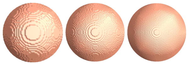
The boundaries extracted from the cubic meshes with the different cube sizes.

Figure 14.

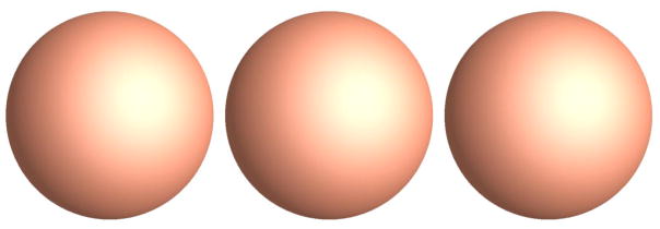
The boundaries extracted from the tetrahedral meshes with the different resolutions.

4.2.2. Comparison of the Thickness Measurement

As we know, the streamline from the methods (Jones et al., 2000; Chung et al., 2007) is obtained by solving laplace equation under the condition of the equilibrium state, (i.e. ${\mathrm{\Delta }}_{M}f(x,t)=\frac{\partial f(x,t)}{\partial t}$, the right of the equation equal to zero). When we move from a vertex point on the outer surface to the next point according to the computed gradient direction and the step length, the next point usually is not a vertex of the digitalized mesh. Then the temperature value of this point needs to be interpolated. Whatever interpolation method, such as the nearest neighbor interpolation, linear interpolation or the cubic spline interpolation, there usually introduce digital errors and result in some accumulated errors for the gradient direction estimation. As a result, the final computed streamlines will be generally different from the ground truth gradient lines. Moreover, the region between the object boundary and the spherical surface is constructed by the cubic voxel. Then the accuracy of tracing the gradient of the equilibrium state is decreased to some extent. In addition, the method needs the binary object whose shape is close to either star-shape or convex. For shapes with a more complex structure, the gradient lines that corresponding to neighboring nodes on the surface will fall within one voxel in the volume, creating numerical singularities in mapping to the sphere. In contrast, our streamline is tracing the maximum transition probability from the specific point x on an isothermal surface to a different point y on the next isothermal surface. The Eq. 5 is considering both the transition probability and more intrinsic geometry structures in the tetrahedron mesh. Because the Eq. 5 contains the eigenvalues and eigenfunctions of the Laplace-Beltrami operator. The following is the details of the comparisons. First, We reconstructed a 3D voxel-based mesh from the boundaries of Fig. 8(a) based on the 3D voxel grid. The boundaries contain an outer boundary which is a cubic surface and an inner boundary which is a sphere surface. At first, we generated the 3D voxel-based volumetric mesh through the binvox software. The mesh contains 31757 uniform cubic voxels comparison to the tetrahedral mesh in Fig. 8 which contains 12360 tetrahedrons. Fig. 15(a) shows the inner boundary (spherical surface) in Fig. 8(a) and Fig. 15(b) shows the generated 3D voxel grid mesh of (a). Though the number of the cubic voxels is bigger than the number of the tetrahedrons, we can see that the boundary mesh in (b) is not as smooth as the one in (a). The slice of the total boundaries of the 3D volumetric grid mesh is shown in Fig. 15(c). The inner boundary of spherical surface is not smooth which can lead to the inaccurate thickness measurement. Also so many cubic voxels will lead to increase the complexity of the finite difference computation.

Figure 15.

The constructed 3D volumetric grid mesh from the inner boundary of Fig. 8(a). Fig. 15(a) shows the spherical boundary and (b) shows the generated 3D voxel grid mesh of Fig. 15(a). (c) shows a slice of the total boundaries of the 3D volumetric grid mesh. And (d) shows the color map of the computed thickness values based on the finite difference method.

Then we set the temperature value of all the outer surfaces as 1° and inner surfaces as 0°. With the volumetric finite difference method, the temperature distribution under the condition of thermal equilibrium and the isothermal surfaces in the mesh can be acquired. The isothermal surfaces are shown in Fig. 16 from left to right, the temperatures are 0.8°, 0.7°, 0.5° and 0.4° respectively. Compared with Fig. 8, the isothermal surfaces from the 3D voxel grid mesh are coarser than the tetrahedral mesh. We found that there are some circular discontinuity regions in every surface. These phenomena are caused by the discontinuity of the internal spherical surface as shown in Fig. 15(b). Next we compute the streamline from the specific sampling point on the outer surface m to the point on the inner surface by the finite difference method. Fig. 15(a) shows the color map of the computed thickness values. The phenomenon of discontinuity still exists. When the resolution is increased, this phenomenon will be somewhat reduced. However, this will bring the high computational complexity. The key reason is that the generated volumetric mesh based on the 3D voxel grid is difficult to fit the original smooth curved surface. While in Fig. 8(d), the color is changing gradually and the phenomenon of discontinuity in Fig. 15(d) is disappear.

Figure 16.

The isothermal surfaces of 0.8°, 0.7°, 0.5° and 0.4° are shown from left to right.

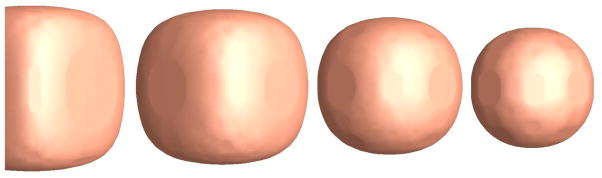
In addition, we use the same outer and inner surface as shown in Fig. 8(a) to reconstruct the new tetrahedral mesh. The difference between the two tetrahedral meshes is that the tetrahedral maxvol in Fig. 17(a) is 0.3 and 0.6 in Fig. 8(a). So the tetrahedral number in Fig. 17(a) is 21379 and the node number is 6581, the tetrahedral number in Fig. 8(a) is 12360 and the node number is 4252. We choose the same step size as 0.01 and the thickness measurement results is shown in Fig. 17(b). Because the number and position of the outer surface points in Fig. 17(b) is different from Fig. 8(d). The thickness colormap is somewhat difference. In order to compare the absolute thickness difference at the same point position between the two measurement results, we get the thickness results according to the points on the outer surface in Fig. 8(d) by interpolating algorithm to Fig. 17(b). Then the thickness differences between the two surface points are shown in Fig. 17(c). There are 633 points in total on the outer surface, about 240 points have the difference, and the maximum of the thickness difference is 0.018. As the interpolation error is excluded, the thickness measurement algorithm is robust under the condition of the different resolution.

Figure 17.

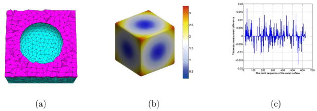
The thickness measurement comparison between the different tetrahedral resolution. (a) is the reconstructed tetrahedral mesh with higher resolution, (b) is the thickness measurement result, and (c) is the thickness differences between the two surface of the different resolution.

In additon, the resolution of the tetrahedral mesh and the time interval of the heat transition will affect the measurement accuracy. In the following, we will discuss the influence of the two factors on these cortical thickness estimation results.

4.3. Influence of the Tetrahedral mesh resolution

In our experiments, we formed the tetrahedrons from the cubic voxels with an edge length of 0.2mm. Similar to classical numerical analysis of finite element methods (e.g. Tsukerman, 1998), the resolution of the tetrahedral mesh will affect the numerical accuracy. Here we adjusted the cubic edge length from 0.15mm to 0.35mm. Statistical p-map results with the heat diffusion thickness measures of different cubic edge length on surface templates representing group differences among two different groups (AD-CTL) are shown in Fig. 18. Non-blue colors show vertices with statistical differences, uncorrected. Fig. 18(a)–(e) are the results of cubic edge length of 0.15, 0.20, 0.25, 0.30 and 0.35mm on group difference between AD and control, respectively. The cumulative distributions of p-values comparison for difference detected between AD and CTL are shown in Fig. 18(f). Their q-values are shown in Table 3. In a total of 5 comparisons, the heat diffusion method of cubic edge length with 0.15 and 0.20mm achieved the highest two q-values. Undoubtedly, the higher the mesh resolution can increase the thickness estimation accuracy, then improve the statistical power. However, the computational complexity will also increase. Considering from the perspectives of computational accuracy and efficiency, we choose the cubic edge length as 0.20mm.

Figure 18.

Statistical p-map results with the heat diffusion thickness measures of different cubic edge length on surface templates representing group differences among two different groups (AD-CTL), of AD subjects (N=51) and control subjects (N=55). Non-blue colors show vertices with statistical differences, uncorrected, (a)–(e) are the results of cubic edge length of 0.15, 0.20, 0.25, 0.30 and 0.35mm on group difference between AD and control, respectively. The cumulative distributions of p-values comparison for difference detected between AD and CTL are shown in (f). The q-values for these maps are shown in Table 3.

Table 3.

The FDR corrected p-values (q-values) comparison with different cubic edge length selections. With the refined cubic edge length, the group difference between AD and healthy control groups demonstrates increased statistical power. The p-maps and CDF are shown in Fig. 18.

Cubic edge length (mm)	q-value
0.15	0.03857
0.20	0.03850
0.25	0.03756
0.30	0.03652
0.35	0.03509

From the Fig. 18, we also find that the significance differences of the different cubic edge length are mainly concentrated in the highly folding area. It is reasonable because these thin areas are modeled better only with refined tetrahedral meshes which consist of shorter cubic lengths.

4.4. Influence of the Heat Transition Time Interval

The l_t(x,y) of the specific point x on an isothermal surface m to the different point y on the next isothermal surface m′ at the same time interval has been computed in Section 3.1 (Fig. 7). At that time we choose the time interval as 0.02. As we know, the l_t(x, y) can also be considered as the amount of heat that is transferred from x to y in time t given a unit heat source at x. Based on the thermodynamic conduction law, the heat of a specific point on the higher temperature isosurface will spread to the point on the lower temperature isosurface along the gradient direction with the largest probability. The time factor t decides the scope of the heat acceptance on the lower temperature isosurface, i.e. the smaller the time, the smaller the range of heat propagation. So the choice of heat transition time interval can influence the heat gradient direction and then the thickness estimation accuracy.

The heat transfer probabilities from the specific point on the higher temperature 0.95° to the lower temperature isosurface 0.90° within the different time interval are shown in Fig. 19(a). With the increased time scale, the heat acceptance difference between the point along the gradient direction and other points around gradually decreases. When the time factor is taken as 0.2, the heat acceptance difference between the point along the gradient direction and other points around is equal to zero. Then it is difficult to find the largest probability direction which represents the gradient direction. Fig. 19(b) shows the heat acceptance results on the lower temperature isosurface with the different time interval. The top left and right are the time interval of 0.02 and 0.03, the bottom left and right are the time interval of 0.04 and 0.2. According to Sun et al. (2009), we choose the minimum time interval as

Figure 19.

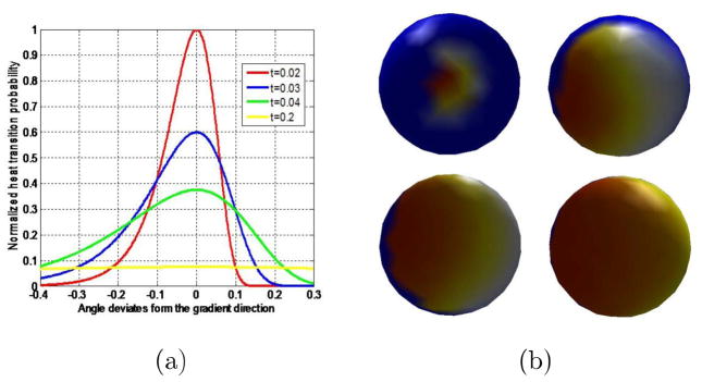
Influence effect of heat transfer time interval. (a) shows the relationships between normalized heat transfer probabilities from the specific point on the higher temperature isosurface (0.95°) to the points on the lower temperature (0.90°) and the angle deviates from the gradient direction. The curves with different colors represent the different heat transfer time intervals. (b) shows the heat acceptance results on the lower temperature isosurface with the different time interval. The top left and right are the time interval of 0.02 and 0.03, the bottom left and right are the time interval of 0.04 and 0.2.

$$t_{min}=\mathit{abs}(4log(10)/{\lambda }_{\mathit{max}})$$ (22)

where the λ_max are the chosen maximum eigenvalues of the Laplace-Beltrami operator. In this paper, in order to obtain the accurate temperature field gradient line, we choose the minimum time interval as 0.02.

In medical imaging field, there are various research involving the thickness estimation, e.g. 3D cell shape analysis (Nandakumar et al., 2011, 2012), 3D corpus collosum thickness estimation (Adamson et al., 2011; Xu et al., 2013b), etc. The proposed algorithm is very general and may be applied to compute any biological structure thickness as long as there are two well-defined boundary surfaces. Starting from our prior work on these techniques (Wang et al., 2004a), here we show that the proposed heat kernel method can be adopted to compute the cortical thickness accurately. Besides the computational efficacy and efficiency, our method also enjoys numerous other advantages of the spectral analysis, e.g., it is physically natural and its computation is numerically stable. We hope our work can provide some practical experience and inspire more interest in 3D heat kernel related research in medical imaging analysis society.

5. Conclusion

In this paper, we present a heat kernel based thickness estimation algorithm which can improve the computational efficiency and accuracy for in vivo MR image cortical thickness estimation. Through establishing the tetrahedral mesh matching with the MRI by the harmonic energy function, we can reduce the limited grid resolution effects. At the same time, we introduce the heat kernel to the streamline analysis to determine the heat transferring gradient direction. With the proposed univariate statistics, we studied differences between three diagnostic groups: AD, MCI and control. We compared our method with the FreeSurfer software, the empirical results demonstrated the potential that the heat diffusion method may achieve greater statistical power than the FreeSurfer software in a total of three comparisons. In the future, we plan to apply our heat kernel diffusion algorithm to depict the geometrical characteristics of the local and global cortical regions and apply them in our ongoing preclinical AD research (Caselli and Reiman, 2013; Langbaum et al., 2013).

Research Highlights.

• A high-quality tetrahedral mesh suitable to represent cortical structures

• A volumetric Laplace-Beltrami operator to achieve the sub-voxel accuracy with a strong theoretic guarantee

• A heat kernel based method to accurately estimate the streamlines with intrinsic and global geometry information

• A novel data structure, half-face structure, for efficient tetrahedral mesh access

• Experiments on synthetic and ADNI data showed promising results

References

- Adamson CL, Wood AG, Chen J, Barton S, Reutens DC, Pantelis C, Velakoulis D, Walterfang M. Thickness profile generation for the corpus callosum using Laplace’s equation. Hum Brain Mapp. 2011;32:2131–2140. doi: 10.1002/hbm.21174. [DOI] [PMC free article] [PubMed] [Google Scholar]
- Alzheimer’s Association. Alzheimer’s disease facts and figures. Alzheimer’s Association; 2012. http://www.alz.org. [DOI] [PubMed] [Google Scholar]
- Benjamini Y, Hochberg Y. Controlling the False Discovery Rate: A Practical and Powerful Approach to Multiple Testing. Journal of the Royal Statistical Society Series B (Methodological) 1995;57:289–300. [Google Scholar]
- Berg L. Clinical Dementia Rating (CDR) Psychopharmacol Bull. 1988;24:637–639. [PubMed] [Google Scholar]
- Braak H, Braak E. Neuropathological stageing of Alzheimer-related changes. Acta Neuropathol. 1991;82:239–259. doi: 10.1007/BF00308809. [DOI] [PubMed] [Google Scholar]
- Braskie MN, Thompson PM. A Focus on Structural Brain Imaging in the Alzheimer’s Disease Neuroimaging Initiative. Biol Psychiatry. 2013 doi: 10.1016/j.biopsych.2013.11.020. [DOI] [PMC free article] [PubMed] [Google Scholar]
- Bronstein MM, Bronstein AM. Shape recognition with spectral distances. IEEE Trans Pattern Anal Mach Intell. 2011;33:1065–1071. doi: 10.1109/TPAMI.2010.210. [DOI] [PubMed] [Google Scholar]
- Cardenas VA, Chao LL, Studholme C, Yaffe K, Miller BL, Madison C, Buckley ST, Mungas D, Schuff N, Weiner MW. Brain atrophy associated with baseline and longitudinal measures of cognition. Neurobiol Aging. 2011;32:572–580. doi: 10.1016/j.neurobiolaging.2009.04.011. [DOI] [PMC free article] [PubMed] [Google Scholar]
- Cardoso MJ, Clarkson MJ, Ridgway GR, Modat M, Fox NC, Ourselin S. LoAd: a locally adaptive cortical segmentation algorithm. Neuroimage. 2011;56:1386–1397. doi: 10.1016/j.neuroimage.2011.02.013. [DOI] [PMC free article] [PubMed] [Google Scholar]
- Caselli RJ, Reiman EM. Characterizing the preclinical stages of Alzheimer’s disease and the prospect of presymptomatic intervention. J Alzheimers Dis. 2013;33(Suppl 1):S405–416. doi: 10.3233/JAD-2012-129026. [DOI] [PMC free article] [PubMed] [Google Scholar]
- Cassidy J, Lilge L, Betz V. Fullmonte: a framework for high-performance monte carlo simulation of light through turbid media with complex geometry. Proc. SPIE; 2013. pp. 85920H–85920H–14. [Google Scholar]
- CGAL Editorial Board. Cgal, Computational Geometry Algorithms Library. 2013 Http://www.cgal.org.
- Chen K, Reiman EM, Alexander GE, Caselli RJ, Gerkin R, Bandy D, Domb A, Osborne D, Fox N, Crum WR, Saunders AM, Hardy J. Correlations between apolipoprotein E epsilon4 gene dose and whole brain atrophy rates. Am J Psychiatry. 2007;164:916–921. doi: 10.1176/ajp.2007.164.6.916. [DOI] [PubMed] [Google Scholar]
- Chung M, Dalton K, Shen L, Evans A, Davidson R. Weighted Fourier representation and its application to quantifying the amount of gray matter. IEEE Transactions on Medical Imaging. 2007;26:566–581. doi: 10.1109/TMI.2007.892519. [DOI] [PubMed] [Google Scholar]
- Chung MK. Computational Neuroanatomy: The Methods. World Scientific Publishing Company; 2012. [Google Scholar]
- Chung MK, Robbins SM, Dalton KM, Davidson RJ, Alexander AL, Evans AC. Cortical thickness analysis in autism with heat kernel smoothing. NeuroImage. 2005;25:1256–1265. doi: 10.1016/j.neuroimage.2004.12.052. [DOI] [PubMed] [Google Scholar]
- Clarkson MJ, Cardoso MJ, Ridgway GR, Modat M, Leung KK, Rohrer JD, Fox NC, Ourselin S. A comparison of voxel and surface based cortical thickness estimation methods. Neuroimage. 2011;57:856–865. doi: 10.1016/j.neuroimage.2011.05.053. [DOI] [PubMed] [Google Scholar]
- Coifman RR, Lafon S, Lee AB, Maggioni M, Nadler B, Warner F, Zucker SW. Geometric diffusions as a tool for harmonic analysis and structure definition of data: diffusion maps. Proc Natl Acad Sci USA. 2005a;102:7426–7431. doi: 10.1073/pnas.0500334102. [DOI] [PMC free article] [PubMed] [Google Scholar]
- Coifman RR, Lafon S, Lee AB, Maggioni M, Nadler B, Warner F, Zucker SW. Geometric diffusions as a tool for harmonic analysis and structure definition of data: multiscale methods. Proc Natl Acad Sci USA. 2005b;102:7432–7437. doi: 10.1073/pnas.0500896102. [DOI] [PMC free article] [PubMed] [Google Scholar]
- Dahnke R, Yotter RA, Gaser C. Cortical thickness and central surface estimation. Neuroimage. 2013;65:336–348. doi: 10.1016/j.neuroimage.2012.09.050. [DOI] [PubMed] [Google Scholar]
- Dale AM, Fischl B, Sereno MI. Cortical surface-based analysis. I. Segmentation and surface reconstruction. Neuroimage. 1999;9:179–194. doi: 10.1006/nimg.1998.0395. [DOI] [PubMed] [Google Scholar]
- Das SR, Avants BB, Grossman M, Gee JC. Registration based cortical thickness measurement. Neuroimage. 2009;45:867–879. doi: 10.1016/j.neuroimage.2008.12.016. [DOI] [PMC free article] [PubMed] [Google Scholar]
- Davatzikos C. Spatial transformation and registration of brain images using elastically deformable models. Comput Vis Image Understanding. 1997;66:207–222. doi: 10.1006/cviu.1997.0605. [DOI] [PubMed] [Google Scholar]
- Desikan RS, Segonne F, Fischl B, Quinn BT, Dickerson BC, Blacker D, Buckner RL, Dale AM, Maguire RP, Hyman BT, Albert MS, Killiany RJ. An automated labeling system for subdividing the human cerebral cortex on MRI scans into gyral based regions of interest. Neuroimage. 2006;31:968–980. doi: 10.1016/j.neuroimage.2006.01.021. [DOI] [PubMed] [Google Scholar]
- Fang Q, Boas DA. Tetrahedral mesh generation from volumetric binary and grayscale images. 2009. pp. 1142–1145. [Google Scholar]
- Fischl B, Dale AM. Measuring the thickness of the human cerebral cortex from magnetic resonance images. Proc Natl Acad Sci USA. 2000;97:11050–11055. doi: 10.1073/pnas.200033797. [DOI] [PMC free article] [PubMed] [Google Scholar]
- Fischl B, Sereno MI, Dale AM. Cortical surface-based analysis. II: Inflation, flattening, and a surface-based coordinate system. Neuroimage. 1999a;9:195–207. doi: 10.1006/nimg.1998.0396. [DOI] [PubMed] [Google Scholar]
- Fischl B, Sereno MI, Tootell RB, Dale AM. High-resolution intersubject averaging and a coordinate system for the cortical surface. Hum Brain Mapp. 1999b;8:272–284. doi: 10.1002/(SICI)1097-0193(1999)8:4<272::AID-HBM10>3.0.CO;2-4. [DOI] [PMC free article] [PubMed] [Google Scholar]
- Folstein MF, Folstein SE, McHugh PR. “Mini-mental state”. A practical method for grading the cognitive state of patients for the clinician. J Psychiatr Res. 1975;12:189–198. doi: 10.1016/0022-3956(75)90026-6. [DOI] [PubMed] [Google Scholar]
- Fox NC, Scahill RI, Crum WR, Rossor MN. Correlation between rates of brain atrophy and cognitive decline in AD. Neurology. 1999;52:1687–1689. doi: 10.1212/wnl.52.8.1687. [DOI] [PubMed] [Google Scholar]
- Frisoni GB, Fox NC, Jack CR, Scheltens P, Thompson PM. The clinical use of structural MRI in Alzheimer disease. Nat Rev Neurol. 2010;6:67–77. doi: 10.1038/nrneurol.2009.215. [DOI] [PMC free article] [PubMed] [Google Scholar]
- Gelb A. The resolution of the gibbs phenomenon for spherical harmonics. Mathematics of Computation. 1997;66:699–717. [Google Scholar]
- Gonzalez O, Stuart A. A First Course in Continuum Mechanics. Cambridge University Press; Cambridge: 2008. [Google Scholar]
- Gu X, Wang Y, Chan T, Thompson T, Yau S. Genus zero surface conformal mapping and its application to brain surface mapping. IEEE Transaction on Medical Imaging. 2004;23:1–10. doi: 10.1109/TMI.2004.831226. [DOI] [PubMed] [Google Scholar]
- den Heijer T, van der Lijn F, Koudstaal PJ, Hofman A, van der Lugt A, Krestin GP, Niessen WJ, Breteler MM. A 10-year follow-up of hippocampal volume on magnetic resonance imaging in early dementia and cognitive decline. Brain. 2010;133:1163–1172. doi: 10.1093/brain/awq048. [DOI] [PubMed] [Google Scholar]
- Hsu EP. Stochastic Analysis on Manifolds. American Mathematical Society; 2002. [Google Scholar]
- Hua X, Lee S, Hibar DP, Yanovsky I, Leow AD, Toga AW, Jack CR, Bernstein MA, Reiman EM, Harvey DJ, Kornak J, Schuff N, Alexander GE, Weiner MW, Thompson PM. Mapping Alzheimer’s disease progression in 1309 MRI scans: power estimates for different inter-scan intervals. Neuroimage. 2010;51:63–75. doi: 10.1016/j.neuroimage.2010.01.104. [DOI] [PMC free article] [PubMed] [Google Scholar]
- Hyde DE, Duffy FH, Warfield SK. Anisotropic partial volume CSF modeling for EEG source localization. Neuroimage. 2012;62:2161–2170. doi: 10.1016/j.neuroimage.2012.05.055. [DOI] [PMC free article] [PubMed] [Google Scholar]
- Jack CR, Bernstein MA, Fox NC, Thompson P, Alexander G, Harvey D, Borowski B, Britson PJ, Whitwell LJ, Ward C, Dale AM, Felmlee JP, Gunter JL, Hill DL, Killiany R, Schuff N, Fox-Bosetti S, Lin C, Studholme C, DeCarli CS, Krueger G, Ward HA, Metzger GJ, Scott KT, Mallozzi R, Blezek D, Levy J, Debbins JP, Fleisher AS, Albert M, Green R, Bartzokis G, Glover G, Mugler J, Weiner MW. The Alzheimer’s Disease Neuroimaging Initiative (ADNI): MRI methods. J Magn Reson Imaging. 2008;27:685–691. doi: 10.1002/jmri.21049. [DOI] [PMC free article] [PubMed] [Google Scholar]
- Jack CR, Slomkowski M, Gracon S, Hoover TM, Felmlee JP, Stewart K, Xu Y, Shiung M, O’Brien PC, Cha R, Knopman D, Petersen RC. MRI as a biomarker of disease progression in a therapeutic trial of milameline for AD. Neurology. 2003;60:253–260. doi: 10.1212/01.wnl.0000042480.86872.03. [DOI] [PMC free article] [PubMed] [Google Scholar]
- Jones G, Chapman S. Modeling growth in biological materials. SIAM Review. 2012;54:52–118. [Google Scholar]
- Jones SE, Buchbinder BR, Aharon I. Three-dimensional mapping of cortical thickness using Laplace’s equation. Hum Brain Mapp. 2000;11:12–32. doi: 10.1002/1097-0193(200009)11:1<12::AID-HBM20>3.0.CO;2-K. [DOI] [PMC free article] [PubMed] [Google Scholar]
- Joshi AA, Ashrafulla S, Shattuck DW, Damasio H, Leahy RM. An invariant shape representation using the anisotropic Helmholtz equation. Med Image Comput Comput Assist Interv. 2012;15:607–614. doi: 10.1007/978-3-642-33454-2_75. [DOI] [PMC free article] [PubMed] [Google Scholar]
- Kabani N, Le Goualher G, MacDonald D, Evans AC. Measurement of cortical thickness using an automated 3-D algorithm: a validation study. Neuroimage. 2001;13:375–380. doi: 10.1006/nimg.2000.0652. [DOI] [PubMed] [Google Scholar]
- Kettner L. Using generic programming for designing a data structure for polyhedral surfaces. Comput Geom Theory Appl. 1999;13:65–90. [Google Scholar]
- Kochunov P, Rogers W, Mangin JF, Lancaster J. A library of cortical morphology analysis tools to study development, aging and genetics of cerebral cortex. Neuroinformatics. 2012;10:81–96. doi: 10.1007/s12021-011-9127-9. [DOI] [PMC free article] [PubMed] [Google Scholar]
- Kremer M. Openvolumemesh - a generic and versatile index-based data structure for polytopal meshes. 2011 http://www.openvolumemesh.org/index.php?id=418.
- Krizek M. On the Maximum Angle Condition for Linear Tetrahedral Elements. SIAM Journal on Numerical Analysis. 1992;29:513–520. [Google Scholar]
- Langbaum JB, Fleisher AS, Chen K, Ayutyanont N, Lopera F, Quiroz YT, Caselli RJ, Tariot PN, Reiman EM. Ushering in the study and treatment of preclinical Alzheimer disease. Nat Rev Neurol. 2013;9:371–381. doi: 10.1038/nrneurol.2013.107. [DOI] [PMC free article] [PubMed] [Google Scholar]
- Lederman C, Joshi A, Dinov I. Tetrahedral mesh generation for medical images with multiple regions using active surfaces. Proc IEEE Int Symp Biomed Imaging; 2010. pp. 436–439. [DOI] [PMC free article] [PubMed] [Google Scholar]
- Lederman C, Joshi A, Dinov I, Vese L, Toga A, Van Horn JD. The generation of tetrahedral mesh models for neuroanatomical MRI. Neuroimage. 2011;55:153–164. doi: 10.1016/j.neuroimage.2010.11.013. [DOI] [PMC free article] [PubMed] [Google Scholar]
- Li B, Li X, Wang K, Qin H. Surface mesh to volumetric spline conversion with generalized polycubes. Visualization and Computer Graphics, IEEE Transactions on. 2013;19:1539–1551. doi: 10.1109/TVCG.2012.177. [DOI] [PubMed] [Google Scholar]
- Li X, Guo X, Wang H, He Y, Gu X, Qin H. Harmonic volumetric mapping for solid modeling applications. Proceedings of the 2007 ACM symposium on Solid and physical modeling; New York, NY, USA: ACM; 2007. pp. 109–120. [Google Scholar]
- Li X, Xu H, Wan S, Yin Z, Yu W. Feature-aligned harmonic volumetric mapping using MFS. Computers & Graphics. 2010;34:242–251. [Google Scholar]
- Litman R, Bronstein AM. Learning spectral descriptors for deformable shape correspondence. IEEE Trans Pattern Anal Mach Intell. 2014;36:171–180. doi: 10.1109/TPAMI.2013.148. [DOI] [PubMed] [Google Scholar]
- Liu Y, Foteinos PA, Chernikov AN, Chrisochoides N. Mesh deformation-based multi-tissue mesh generation for brain images. Eng Comput (Lond ) 2012;28:305–318. [Google Scholar]
- Liu Y, Xing H. A boundary focused quadrilateral mesh generation algorithm for multi-material structures. Journal of Computational Physics. 2013;232:516–528. [Google Scholar]
- Lombaert H, Grady L, Polimeni JR, Cheriet F. IEEE Trans Pattern Anal Mach Intell. 2012. FOCUSR: Feature Oriented Correspondence using Spectral Regularization - A Method for Accurate Surface Matching. [DOI] [PMC free article] [PubMed] [Google Scholar]
- MacDonald D, Kabani N, Avis D, Evans AC. Automated 3-D extraction of inner and outer surfaces of cerebral cortex from MRI. Neuroimage. 2000;12:340–356. doi: 10.1006/nimg.1999.0534. [DOI] [PubMed] [Google Scholar]
- Mak-Fan KM, Taylor MJ, Roberts W, Lerch JP. Measures of cortical grey matter structure and development in children with autism spectrum disorder. J Autism Dev Disord. 2012;42:419–427. doi: 10.1007/s10803-011-1261-6. [DOI] [PubMed] [Google Scholar]
- MakeHuman Project Team. MakeHuman project. 2013 http://makehuman.sourceforge.net/API/halfedges-module.html.
- Mäntylä M. An Introduction to Solid Modeling. Computer Science Press; Rockville, MD: 1988. [Google Scholar]
- Miller MI, Massie AB, Ratnanather JT, Botteron KN, Csernansky JG. Bayesian construction of geometrically based cortical thickness metrics. Neuroimage. 2000;12:676–687. doi: 10.1006/nimg.2000.0666. [DOI] [PubMed] [Google Scholar]
- Min P. [binvox] 3d mesh voxelizer. 2013 http://www.google.com/search?q=binvox.
- Mueller SG, Weiner MW, Thal LJ, Petersen RC, Jack C, Jagust W, Trojanowski JQ, Toga AW, Beckett L. The Alzheimer’s disease neuroimaging initiative. Neuroimaging Clin N Am. 2005;15:869–877. doi: 10.1016/j.nic.2005.09.008. [DOI] [PMC free article] [PubMed] [Google Scholar]
- Nandakumar V, An X, Wang Y, Johnson R, Meldrum D. Conformal mapping of nuclei in 3d tomographic cell images to assess shape heterogeneity. Biomedical Imaging (ISBI), 2012 9th IEEE International Symposium on; 2012. pp. 222–225. [Google Scholar]
- Nandakumar V, Kelbauskas L, Johnson R, Meldrum D. Quantitative characterization of preneoplastic progression using single-cell computed tomography and three-dimensional karyometry. Cytometry A. 2011;79:25–34. doi: 10.1002/cyto.a.20997. [DOI] [PMC free article] [PubMed] [Google Scholar]
- Nichols T, Hayasaka S. Controlling the familywise error rate in functional neuroimaging: a comparative review. Stat Methods Med Res. 2003;12:419–446. doi: 10.1191/0962280203sm341ra. [DOI] [PubMed] [Google Scholar]
- Nooruddin FS, Turk G. Simplification and repair of polygonal models using volumetric techniques. IEEE Trans on Vis and Comput Graph. 2003;9:191–205. [Google Scholar]
- Pai D, Soltanian-Zadeh H, Hua J. Evaluation of fiber bundles across subjects through brain mapping and registration of diffusion tensor data. Neuroimage. 2011;54(Suppl 1):S165–175. doi: 10.1016/j.neuroimage.2010.05.085. [DOI] [PubMed] [Google Scholar]
- Paillé GP, Poulin P. As-conformal-as-possible discrete volumetric mapping. Computers & Graphics. 2012;36:427–433. [Google Scholar]
- Pedegral P. Variational Methods in Nonlinear Elasticity. Society for industrial Mathematics; Philadelphia: 2000. [Google Scholar]
- Qiu A, Bitouk D, Miller MI. Smooth functional and structural maps on the neocortex via orthonormal bases of the Laplace-Beltrami operator. IEEE Trans Med Imaging. 2006a;25:1296–1306. doi: 10.1109/tmi.2006.882143. [DOI] [PubMed] [Google Scholar]
- Qiu A, Rosenau BJ, Greenberg AS, Hurdal MK, Barta P, Yantis S, Miller MI. Estimating linear cortical magnification in human primary visual cortex via dynamic programming. Neuroimage. 2006b;31:125–138. doi: 10.1016/j.neuroimage.2005.11.049. [DOI] [PubMed] [Google Scholar]
- Raviv D, Bronstein MM, Bronstein AM, Kimmel R. Volumetric heat kernel signatures. Proc. Intl. Workshop on 3D Object Retrieval (3DOR), ACM Multimedia; 2010. pp. 39–44. [Google Scholar]
- Reiman EM, Uecker A, Caselli RJ, Lewis S, Bandy D, de Leon MJ, De Santi S, Convit A, Osborne D, Weaver A, Thibodeau SN. Hippocampal volumes in cognitively normal persons at genetic risk for Alzheimer’s disease. Ann Neurol. 1998;44:288–291. doi: 10.1002/ana.410440226. [DOI] [PubMed] [Google Scholar]
- Rustamov RM. Interpolated eigenfunctions for volumetric shape processing. Vis Comput. 2011;27:951–961. [Google Scholar]
- Sethian JA. A fast marching level set method for monotonically advancing fronts. Proc Natl Acad Sci USA. 1996;93:1591–1595. doi: 10.1073/pnas.93.4.1591. [DOI] [PMC free article] [PubMed] [Google Scholar]
- Sharma A, Horaud RP, Mateus D. 3D shape registration using spectral graph embedding and probabilistic matching. Image Processing and Analysing With Graphs: Theory and Practice. 2012:441–474. [Google Scholar]
- Shewchuk JR. What is a good Linear Element? Interpolation, Conditioning, and Quality Measures. In Eleventh International Meshing Roundtable; 2002. pp. 115–126. [Google Scholar]
- Shi J, Thompson PM, Gutman B, Wang Y. Surface fluid registration of conformal representation: application to detect disease burden and genetic influence on hippocampus. Neuroimage. 2013a;78:111–134. doi: 10.1016/j.neuroimage.2013.04.018. [DOI] [PMC free article] [PubMed] [Google Scholar]
- Shi Y, Lai R, Morra JH, Dinov I, Thompson PM, Toga AW. Robust surface reconstruction via Laplace-Beltrami eigen-projection and boundary deformation. IEEE Trans Med Imaging. 2010;29:2009–2022. doi: 10.1109/TMI.2010.2057441. [DOI] [PMC free article] [PubMed] [Google Scholar]
- Shi Y, Lai R, Toga AW. Cortical surface reconstruction via unified Reeb analysis of geometric and topological outliers in magnetic resonance images. IEEE Trans Med Imaging. 2013b;32:511–530. doi: 10.1109/TMI.2012.2224879. [DOI] [PMC free article] [PubMed] [Google Scholar]
- Si H. Constrained delaunay tetrahedral mesh generation and refinement. Finite Elem Anal Des. 2010;46:33–46. [Google Scholar]
- Sperling RA, Aisen PS, Beckett LA, Bennett DA, Craft S, Fagan AM, Iwatsubo T, Jack CR, Kaye J, Montine TJ, Park DC, Reiman EM, Rowe CC, Siemers E, Stern Y, Yaffe K, Carrillo MC, Thies B, Morrison-Bogorad M, Wagster MV, Phelps CH. Toward defining the preclinical stages of Alzheimer’s disease: recommendations from the National Institute on Aging-Alzheimer’s Association workgroups on diagnostic guidelines for Alzheimer’s disease. Alzheimers Dement. 2011;7:280–292. doi: 10.1016/j.jalz.2011.03.003. [DOI] [PMC free article] [PubMed] [Google Scholar]
- Stonnington CM, Chu C, Kloppel S, Jack CR, Ashburner J, Frackowiak RS. Predicting clinical scores from magnetic resonance scans in Alzheimer’s disease. Neuroimage. 2010;51:1405–1413. doi: 10.1016/j.neuroimage.2010.03.051. [DOI] [PMC free article] [PubMed] [Google Scholar]
- Sun J, Ovsjanikov M, Guibas L. A concise and provably informative multi-scale signature based on heat diffusion. Proceedings of the Symposium on Geometry Processing; Berlin, Germany: Eurographics Association; 2009. pp. 1383–1392. [Google Scholar]
- Tan Y, Hua J, Qin H. Physically based modeling and simulation with dynamic spherical volumetric simplex splines. Computer-Aided Design. 2010;42:95–108. doi: 10.1016/j.cad.2009.02.014. [DOI] [PMC free article] [PubMed] [Google Scholar]
- Thompson PM, Hayashi KM, De Zubicaray GI, Janke AL, Rose SE, Semple J, Hong MS, Herman DH, Gravano D, Doddrell DM, Toga AW. Mapping hippocampal and ventricular change in Alzheimer disease. Neuroimage. 2004;22:1754–1766. doi: 10.1016/j.neuroimage.2004.03.040. [DOI] [PubMed] [Google Scholar]
- Thompson PM, Hayashi KM, de Zubicaray G, Janke AL, Rose SE, Semple J, Herman D, Hong MS, Dittmer SS, Doddrell DM, Toga AW. Dynamics of gray matter loss in Alzheimer’s disease. J Neurosci. 2003;23:994–1005. doi: 10.1523/JNEUROSCI.23-03-00994.2003. [DOI] [PMC free article] [PubMed] [Google Scholar]
- Tsukerman I. A general accuracy criterion for finite element approximation. Magnetics, IEEE Transactions on. 1998;34:2425–2428. [Google Scholar]
- Wang J, Yu Z. Feature-sensituve tetrahedral mesh generation with guaranteed quality. Computer-Aided Design. 2012;44:400–412. doi: 10.1016/j.cad.2012.01.002. [DOI] [PMC free article] [PubMed] [Google Scholar]
- Wang K, Li X, Li B, Xu H, Qin H. Restricted trivariate polycube splines for volumetric data modeling. Visualization and Computer Graphics, IEEE Transactions on. 2012a;18:703–716. doi: 10.1109/TVCG.2011.102. [DOI] [PubMed] [Google Scholar]
- Wang Y, Gu X, Chan TF, Thompson PM, Yau ST. Volumetric harmonic brain mapping. Biomedical Imaging: From Nano to Macro, 2004. ISBI 2004. IEEE International Symposium on; 2004a. pp. 1275–1278. [Google Scholar]
- Wang Y, Gu X, Yau ST. Volumetric harmonic map. Communications in Information and Systems. 2004b;3:191–202. [Google Scholar]
- Wang Y, Shi J, Yin X, Gu X, Chan TF, Yau ST, Toga AW, Thompson PM. Brain surface conformal parameterization with the Ricci flow. IEEE Trans Med Imaging. 2012b;31:251–264. doi: 10.1109/TMI.2011.2168233. [DOI] [PMC free article] [PubMed] [Google Scholar]
- Wang Y, Song Y, Rajagopalan P, An T, Liu K, Chou YY, Gutman B, Toga AW, Thompson PM. Surface-based TBM boosts power to detect disease effects on the brain: an N=804 ADNI study. Neuroimage. 2011;56:1993–2010. doi: 10.1016/j.neuroimage.2011.03.040. [DOI] [PMC free article] [PubMed] [Google Scholar]
- Wechsler D. Wechsler Memory Scale-Revised Manual. Psychological Corporation; San Antonio, TX: 1987. [Google Scholar]
- Wolz R, Heckemann RA, Aljabar P, Hajnal JV, Hammers A, Lotjonen J, Rueckert D. Measurement of hippocampal atrophy using 4D graph-cut segmentation: application to ADNI. Neuroimage. 2010;52:109–118. doi: 10.1016/j.neuroimage.2010.04.006. [DOI] [PubMed] [Google Scholar]
- Xu H, Yu W, Gu S, Li X. Biharmonic volumetric mapping using fundamental solutions. Visualization and Computer Graphics, IEEE Transactions on. 2013a;19:787–798. doi: 10.1109/TVCG.2012.173. [DOI] [PubMed] [Google Scholar]
- Xu L. Master’s thesis. Arizona State University; 2013. Combining Thickness Information with Surface Tensor-based Morphometry for the 3D Statistical Analysis of the Corpus Callosum. [Google Scholar]
- Xu L, Collignon O, Wang G, Kang Y, Leporé F, Shi J, Lao Y, Joshi A, Leporé N, Wang* Y. In: Pennec X, Joshi S, Nielsen M, Fletcher T, Durrleman S, Sommer S, editors. Combining thickness information with surface tensor-based morphometry for the 3d statistical analysis of the corpus callosum; the 4th MICCAI Workshop on Mathematical Foundations of Computational Anatomy (MFCA); Nagoya, Japan. 2013b. pp. 26–36. [Google Scholar]
- Zeng W, Guo R, Luo F, Gu X. Discrete heat kernel determines discrete riemannian metric. Graph Models. 2012;74:121–129. [Google Scholar]
- Zhang Y, Bajaj C, Sohn BS. 3D Finite Element Meshing from Imaging Data. Comput Methods Appl Mech Eng. 2005;194:5083–5106. doi: 10.1016/j.cma.2004.11.026. [DOI] [PMC free article] [PubMed] [Google Scholar]