4D Hyperspherical Harmonic (HyperSPHARM) Representation of Surface Anatomy: A Holistic Treatment of Multiple Disconnected Anatomical Structures

Abstract

Image-based parcellation of the brain often leads to multiple disconnected anatomical structures, which pose significant challenges for analyses of morphological shapes. Existing shape models, such as the widely used spherical harmonic (SPHARM) representation, assume topological invariance, so are unable to simultaneously parameterize multiple disjoint structures. In such a situation, SPHARM has to be applied separately to each individual structure. We present a novel surface parameterization technique using 4D hyperspherical harmonics in representing multiple disjoint objects as a single analytic function, terming it HyperSPHARM. The underlying idea behind Hyper-SPHARM is to stereographically project an entire collection of disjoint 3D objects onto the 4D hypersphere and subsequently simultaneously parameterize them with the 4D hyperspherical harmonics. Hence, HyperSPHARM allows for a holistic treatment of multiple disjoint objects, unlike SPHARM. In an imaging dataset of healthy adult human brains, we apply HyperSPHARM to the hippocampi and amygdalae. The HyperSPHARM representations are employed as a data smoothing technique, while the HyperSPHARM coefficients are utilized in a support vector machine setting for object classification. HyperSPHARM yields nearly identical results as SPHARM, as will be shown in the paper. Its key advantage over SPHARM lies computationally; Hyper-SPHARM possess greater computational efficiency than SPHARM because it can parameterize multiple disjoint structures using much fewer basis functions and stereographic projection obviates SPHARM's burdensome surface flattening. In addition, HyperSPHARM can handle any type of topology, unlike SPHARM, whose analysis is confined to topologically invariant structures.

1. Introduction

Multiple disconnected anatomical structures (MIDAS) refer to two or more structures that are anatomically and/or functionally separate, and their underlying mathematical feature is changing topology (e.g. gaps, holes). Hence, the individual structures forming the MIDAS do not have to be physically connected, as there could be gaps separating the individual structures from each other, and can have holes. Prominent examples include the limbic structures (hippocampi and amygdalae) in the brain and the unfused hyoid bone in the neck. Image-based parcellation of MIDAS poses significant challenges for analyses of morphological shapes; existing shape models assume topological invariance, so can only be applied to a single connected structure. An important problem then is formulating a single, coherent mathematical parameterization that can allow for a holistic treatment of MIDAS, i.e. treating the entire MIDAS as a single entity.

Probably the most widely applied shape parameterization technique for cortical structures is the spherical harmonic (SPHARM) representation (Chung et al., 2010; Gerig et al., 2001; Shen et al., 2004; Gu et al., 2004; Styner et al., 2006), which has been mainly used as a data reduction technique for compressing global shape features into a small number of coefficients. The main global geometric features are encoded in low degree coefficients while the noise will be in high degree spherical harmonics. The method has been used to model various brain structures such as ventricles (Gerig et al., 2001), hippocampi (Shen et al., 2004) and cortical surfaces (Chung et al., 2010; Gu et al., 2004). SPHARM, however, can't represent MIDAS with a single parameterization. In such a situation, SPHARM has to be applied separately to each individual structure forming the MIDAS. In addition, SPHARM-representation requires a 3D anatomical surface to be mapped onto a 3D sphere, which is no simple task. Various computationally intensive surface flattening techniques have been proposed as a result: diffusion mapping (Chung et al., 2010), conformal mapping (Angenent et al., 1999; Gu et al., 2004; Hurdal and Stephenson, 2004), quasi-isometric mapping (Timsari and Leahy, 2000) and area preserving mapping (Gerig et al., 2001; Brechbuhler et al., 1995). The surface flattening is used to parameterize the surface using two spherical angles. The angles serve as coordinates for representing the surface using spherical harmonics. Then the surface coordinates can be mapped onto the sphere and each coordinate is represented as a linear combination of spherical harmonics.

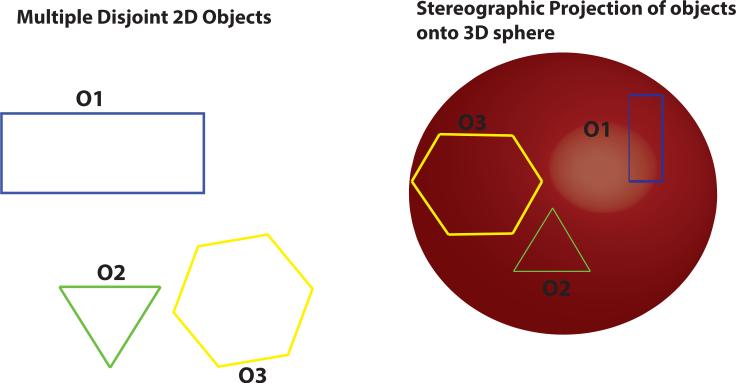
Any 3D object may be embedded onto the surface of a 4D hypersphere via simple stereographic projection. Extending the concept further, two or more disconnected 3D objects may be stereographically projected onto the same 4D hypersphere. Consequently, all the multiple disconnected 3D objects (forming the MIDAS) exist on the same hypersphere, so the entire MIDAS can be represented as the linear combination of 4D hyperspherical harmonics (HSH), which are the multidimensional analogues of the 3D spherical harmonics. In other words, such a procedure enables the entire MIDAS to be treated as a single entity existing along the surface of a 4D hypersphere (see Figure 1 for illustration).

Figure 1. Holistic Treatment of Multiple Disjoint Structures.

The underlying idea of HyperSPHARM is stereographically projecting n-dimensional data onto the (n+1)-dimensional sphere in order to subsequently parameterize the data with the (n+1)-dimensional spherical harmonics. Here we illustrate the n = 2 case. Three disjoint 2D objects are mapped on the 3D sphere. Since each object is unique in 2D, their projections onto the sphere will also be unique. Consequently, all three disjoint objects exist on the same sphere, so according to Fourier analysis they can be simultaneously parameterized by the 3D spherical harmonics. Please note that the shapes’ angles are preserved since stereographic projection is conformal. However, the projected shapes lying on the sphere will experience metric distortion, e.g. the area of the rectangle existing on the sphere is different from that of the rectangle lying on the 2D plane.

The HSH have been mainly confined to quantum chemistry, where their utility first became evident with respect to solving the Schrödinger equation for the hydrogen atom. It had been solved in position-space by Schrödinger, himself, but not in momentum-space, which is related to position-space via the Fourier transform. Sometime later, V. Fock solved the Schrödinger equation for the hydrogen atom directly in momentum-space. In his classic paper (Fock, 1935), Fock stereographically projected 3D momentum-space onto the surface of a 4D unit hypersphere, and after this mapping was made, he was able to show that the eigenfunctions were the 4D HSH. Recently, the HSH have been utilized in a wider array of fields than just quantum chemistry, including computer graphics visualization (Bonvallet et al., 2007) and crystal-lography (Mason and Schuh, 2008). However, as of yet, they have remained elusive for medical imaging.

In this paper, following the approach of Fock, we model multiple disconnected 3D objects in terms of the 4D HSH by stereographically projecting each object's surface coordinates onto the same 4D hypersphere, and label such a representation HyperSPHARM (Hosseinbor et al., 2013). The incorporation of an extra (4^th) dimension via stereographic projection imbues HyperSPHARM with several key advantages over SPHARM:

1. Stereographic projection onto a 4D hypersphere obviates the difficult and time-consuming 3D surface flattening required by SPHARM.

2. HyperSPHARM is not constrained by topological variance, unlike SPHARM. The parameterization of an object containing a hole (e.g. doughnut) or the simultaneous parameterization of multiple disjoint objects is not possible with SPHARM. HyperSPHARM, however, treats MIDAS holistically by representing it with a single (linear) mathematical parameterization, given by the 4D HSH. SPHARM has to be applied separately to each individual structure forming the MIDAS.

3. HyperSPHARM possesses greater computational efficiency than SPHARM because it can more sparsely represent the MIDAS, which we will demonstrate in this paper.

The method is applied to parameterize the MIDAS comprising the left and right hippocampus and amygdala for an imaging dataset of healthy adult human brains. The HyperSPHARM representations are employed as a surface smoothing technique, while the HyperSPHARM coefficients are used in a support vector machine (SVM) setting for gender classification.

The paper is organized as follows: in Section 2, we review the 4D HSH and its properties. In Section 3, we discuss in detail the HyperSPHARM algorithm. Section 4 goes over the imaging dataset used in this study and the necessary image processing steps. In Section 5, we compare Hyper-SPHARM and SPHARM, utilize HyperSPHARM representations as a data smoothing technique, and employ HyperSPHARM coefficients as features of object classification using SVM. Lastly, we discuss our results and future applications of HyperSPHARM in Section 6.

2. 4D Hyperspherical Harmonics

Consider the 4D unit hypersphere S³ existing in ${\mathbb{R}}^4$ that is defined by three angles: the azimuthal angle ϕ, the 3D zenith angle θ, and the 4D zenith angle β. The Laplace-Beltrami operator on S³ is defined as

$${\Delta }_{S^3}=\frac{1}{{\sin }^2\beta }\frac{\partial }{\partial \beta }{\sin }^2\beta \frac{\partial }{\partial \beta }+\frac{1}{{\sin }^2\beta }{\Delta }_{S^2},$$ (1)

where Δ_S2 is the Laplace-Beltrami operator on the unit sphere S². The eigenfuctions of Eq. (1) are the 4D hyperspherical harmonics $Z_{nl}^m(\beta ,\theta ,\varphi )$:

$${\Delta }_{S^3}{Z}_{nl}^m=-l(l+2)Z_{nl}^m.$$

The 4D HSH are defined as (Domokos, 1967)

$$Z_{nl}^m(\beta ,\theta ,\varphi )=2^{l+1∕2}\sqrt{\frac{(n+1)\Gamma (n-l+1)}{\pi \Gamma (n+l+2)}}\Gamma (l+1){\sin }^l\beta C_{n-l}^{l+1}\left(\cos \beta \right)Y_l^m(\theta ,\varphi ),$$ (2)

where Ω = (β, θ, Φ) obey (β ∈ [0, τ], θ ∈ [0, τ], Φ ∈ [0, 2τ]), $C_{n-1}^{l+1}$ are the Gegenbauer (ultra-spherical) polynomials, and $Y_l^m$ are the 3D spherical harmonics. The index n refers to the degree of the HSH and is commonly referred to as the principal quantum number; and the three integers (n, l, m) obey the conditions n = 0, 1, 2, ..., 0 ≤ l ≤ n, and − ≤ l m ≤ l. The number of HSH corresponding to a given degree n is (n+1)² The HSH form an orthonormal basis on the hypersphere, and the normalization condition reads

$${\int }_0^{2\pi }{\int }_0^{\pi }{\int }_0^{\pi }{Z}_{nl}^m\left(\Omega \right)Z_{n^{\prime }{l}^{\prime }}^{m^{\prime }\ast }\left(\Omega \right){\sin }^2\beta \sin \theta d\beta d\theta d\varphi ={\delta }_{m{n}^{\prime }}{\delta }_{l{l}^{\prime }}{\delta }_{m{m}^{\prime }}$$ (3)

The first few 4D HSH are shown in Table 1. The n = 1 4D HSH define a 4D hypersphere of radius $\sqrt{2}∕\pi$. The spherical harmonics of any dimension are discussed in Appendix A.

Table 1.

List of a Few HSH

$Z_{00}^0(\beta ,\theta ,\varphi )=\frac{1}{\pi \sqrt{2}}$	$Z_{10}^0(\beta ,\theta ,\varphi )=\frac{\sqrt{2}}{\pi }\cos \beta$
$Z_{11}^{-1}(\beta ,\theta ,\varphi )=\frac{-\sqrt{2}}{\pi }\sin \beta \sin \theta \sin \varphi$	$Z_{11}^0(\beta ,\theta ,\varphi )=\frac{\sqrt{2}}{\pi }\sin \beta \cos \theta$
$Z_{11}^1(\beta ,\theta ,\varphi )=\frac{-\sqrt{2}}{\pi }\sin \beta \sin \theta \cos \varphi$	$Z_{20}^0(\beta ,\theta ,\varphi )=\frac{1}{\pi \sqrt{2}}(3-4{\sin }^2\beta )$
$Z_{21}^{-1}(\beta ,\theta ,\varphi )=\frac{-\sqrt{3}}{\pi }\sin 2\beta \sin \theta \sin \varphi$	$Z_{21}^0(\beta ,\theta ,\varphi )=\frac{\sqrt{3}}{\pi }\sin 2\beta \cos \theta$

3. HyperSPHARM Algorithm

In this section, we will elaborate on the HyperSPHARM algorithm, which consists of five basic steps: translation, stereographic projection, 4D HSH expansion, linear least squares estimation, and interpolation. Before proceeding, we need to mathematically define the MIDAS.

Suppose some MIDAS is composed of k individual structures. Each structure is assumed to be both 3D finite and compact (i.e. has no singularities) and comprising surface coordinates ${\mathbf{p}}_j=\left({\mathbf{p}}_j^1{\mathbf{p}}_j^2{\mathbf{p}}_j^3\right)$, where j = 1, 2, ..., k. We further assume that each structure's surface coordinates are unique, i.e. no two structures have overlapping coordinates. Denote N_j as the number of mesh vertices forming structure j, which means the dimension of p_j is N_j x 3. Lets combine the surface coordinates of all k structures in order to facilitate a holistic treatment of the MIDAS. Define v = (v¹ v² v³) as the combined 3D surface coordinates across all k structures, where

$$\begin{array}{cc}\hfill {\mathbf{v}}^1=& {({\mathbf{p}}_1^{1T}{\mathbf{p}}_2^{1T}\cdots {\mathbf{p}}_k^{1T})}^T\hfill \\ \hfill {\mathbf{v}}^2=& {({\mathbf{p}}_1^{2T}{\mathbf{p}}_2^{2T}\cdots {\mathbf{p}}_k^{2T})}^T\hfill \\ \hfill {\mathbf{v}}^3=& {({\mathbf{p}}_1^{3T}{\mathbf{p}}_2^{3T}\cdots {\mathbf{p}}_k^{3T})}^T\hfill \end{array}$$

and the symbol T denotes transpose. In other words, the MIDAS's surface coordinates are defined by v. The dimension of v is M x 3, where $M={\sum }_{j=1}^k{N}_j$ is the total number of mesh vertices comprising the 3D MIDAS. We denote each (vector) coordinate component of v as vⁱ, where i = 1, 2, 3.

3.1. Translation

Note that SPHARM and HyperSPHARM are not translation invariant representations, which reduces their goodness of fit. Translating the MIDAS's surface coordinates v closer to the origin (0, 0, 0) improves the accuracy of the fitting. We achieve this shift towards the origin by subtracting each vⁱ by its mean value:

$${\mathbf{s}}^i={\mathbf{v}}^i-\langle {\mathbf{v}}^i\rangle ,$$

where s = (s¹ s² s³) is the M x 3 matrix denoting the MIDAS's shifted surface coordinates and 〈vⁱ〉 is the mean of vⁱ.

3.2. Stereographic Projection of 3D MIDAS’s Surface Coordinates onto 4D Hypersphere

In order to model the MIDAS’s (shifted) surface coordinates with the HSH, we need to map them onto a 4D hypersphere, which can be achieved via stereographic projection (Fock, 1935). The surface coordinates in 3D spherical space are s¹ = r sin θ cos Φ, s² = r sin θ sin Φ, and s³ = r cos Φ, where $r=\sqrt{{\left(s^1\right)}^2+{\left(s^2\right)}^2+{\left(s^3\right)}^2}$. Consider a 4D hypersphere of radius p_o, whose coordinates are defined as

$$\begin{array}{cc}\hfill u_1=& p_o\sin \beta \sin \theta \cos \varphi \hfill \\ \hfill u_2=& p_o\sin \beta \sin \theta \sin \varphi \hfill \\ \hfill u_3=& p_o\sin \beta \cos \theta \hfill \\ \hfill u_4=& p_o\cos \beta .\hfill \end{array}$$

The relationship between (s¹, s², s³) and (u₁, u₂, u₃, u₄), according to stereo-graphic projection, is

$$\begin{array}{cc}\hfill u_1=& \frac{2p_o^2{s}^1}{r^2+p_o^2},u_2=\frac{2p_o^2{s}^2}{r^2+p_o^2},\hfill \\ \hfill u_3=& \frac{2p_o^2{s}^3}{r^2+p_o^2},u_4=\frac{p_o(r^2-p_o^2)}{r^2+p_o^2}\hfill \end{array}$$ (4)

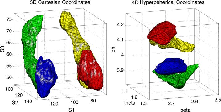
Eq. (4) establishes a one-to-one correspondence between the 3D volume and 4D hypersphere (Fig. 2). As shown in Fig. 2, stereographic projection's inherent lack of volume preservation is not an issue in HyperSPHARM analysis; the projected MIDAS lying on the hypersphere experiences metric distortion, but we are solely interested in the (HyperSPHARM-reconstructed) back-projected MIDAS. We derive stereographic projection to any dimension in Appendix B.

Figure 2.

The 3D subcortical structures (left) in the coordinates (v¹, v², v³) went through the 4D stereographic projection that resulted in conformally deformed structures (right) in the 4D spherical coordinates (β, θ, ϕ). The 3D subcortical structure is then embedded on the surface of the 4D hypersphere with radius p_o = 23.

3.3. HSH Expansion of MIDAS's Surface Coordinates

Stereographically projecting the 3D MIDAS's surface coordinates onto a 4D hypersphere results in them existing along the hypersphere's surface. According to Fourier analysis, any square-integrable function defined on a sphere can be expanded in terms of the spherical harmonics. Thus, we can expand each coordinate component sⁱ in terms of the 4D HSH:

$$s_{p_o}^i(\beta ,\theta ,\varphi )\approx \sum _{n=0}^N\sum _{l=0}^n\sum _{m=-l}^l{C}_{nlm}^i{Z}_{nl}^m(\beta ,\theta ,\varphi ),$$ (5)

where $s_{p_o}^i$ denotes the i^th component of the surface coordinates s existing on hypersphere of radius p_o. The realness of the surface coordinates requires use of the real HSH, so we employ a modified real basis proposed in (Koay et al., 2009) for $Y_l^m$. N is the truncation order of the HSH expansion, and for a given N the total number of HSH expansion coefficients is

$$W=(N+1)(N+2)(2N+3)∕6$$

3.4. Numerical Implementation

Let Ω_j = (β_j, θ_j, ϕ_j) denote the hyperspherical angles at the j-th mesh vertex. Recall that our MIDAS consists of a total of M mesh vertices, so each sⁱ is a M x 1 vector. Denote Cⁱ as the W x 1 vector of unknown HSH expansion coefficients $C_{nlm}^i$ for each sⁱ, and A is M x W matrix constructed with the HSH basis and given by

$$\left(\begin{array}{cccccc}\hfill Z_{00}^0\left({\Omega }_1\right)\hfill & \hfill Z_{10}^0\left({\Omega }_1\right)\hfill & \hfill Z_{11}^{-1}\left({\Omega }_1\right)\hfill & \hfill Z_{11}^0\left({\Omega }_1\right)\hfill & \hfill \cdots \hfill & \hfill Z_{NN}^N\left({\Omega }_1\right)\hfill \\ \hfill ⋮\hfill & \hfill ⋮\hfill & \hfill ⋮\hfill & \hfill ⋮\hfill & \hfill \ddots \hfill & \hfill ⋮\hfill \\ \hfill Z_{00}^0\left({\Omega }_M\right)\hfill & \hfill Z_{10}^0\left({\Omega }_M\right)\hfill & \hfill Z_{11}^{-1}\left({\Omega }_M\right)\hfill & \hfill Z_{11}^0\left({\Omega }_M\right)\hfill & \hfill \cdots \hfill & \hfill Z_{NN}^N\left({\Omega }_M\right)\hfill \end{array}\right).$$

Thus, the general linear system representing Eq. (5) is described by sⁱ = ACⁱ. This system of over-determined equations is solved via linear least squares, yielding

$$\widehat{{\mathbf{C}}^i}={\left({\mathbf{A}}^T\mathbf{A}\right)}^{-1}{\mathbf{A}}^T{\mathbf{s}}^i$$ (6)

The reconstructed (shifted) surface coordinates are then given by $\widehat{{\mathbf{s}}^i}=\mathbf{A}\widehat{{\mathbf{C}}^i}$.

Lastly, we want to estimate the actual surface coordinates v. The recon-structed vⁱ is

$$\widehat{{\mathbf{v}}^i}=\widehat{{\mathbf{s}}^i}+\langle {\mathbf{v}}^i\rangle ,$$ (7)

where we have translated the reconstructed (shifted) surface coordinates back to the original object space. Hence, our reconstructed 3D MIDAS is defined by the M x 3 matrix $\widehat{\mathbf{v}}=\left(\widehat{{\mathbf{v}}^1}\widehat{{\mathbf{v}}^2}\widehat{{\mathbf{v}}^3}\right)$. The mean squared error (MSE) between the original MIDAS and the HyperSPHARM-reconstructed MIDAS can then be computed as

$${\mathrm{MSE}}_{\mathrm{HSH}}=\mathrm{tr}\left[{(\mathbf{v}-\widehat{\mathbf{v}})}^T(\mathbf{v}-\widehat{\mathbf{v}})\right]∕M$$ (8)

3.5. Interpolation

Once the HSH coefficients are estimated by Eq. (6), the surface coordinates of the MIDAS can be evaluated using a different sampling along the 4D hypersphere. Unlike SPHARM, resampling for HyperSPHARM interpolation is not as trivial. Simply resampling points along the 3D MIDAS and then mapping them onto the 4D hypersphere will not work; the mapped samples will not be uniformly distributed along the 4D sphere due to stereographic projection's inherent nonlinearity. We now discuss isotropic sampling along the 4D hypersphere, which we will employ for HyperSPHARM interpolation.

Due to the fact that the stereographic projection of the MIDAS usually lies on some regions of the hyperspherical surface, the evaluation of the surface coordinates of the MIDAS on the 4D hypersphere should be carried out on a sampling that is isotropic on the surface of the 4D hypersphere. The problem of distributing points uniformly on the 3D sphere is a well known problem and was proposed by J. J. Thomson more than a century ago (Thomson, 1904). Variants of the Thomson problem that incorporate antipodal symmetry and mirror-reflection symmetry have been found useful in other scientific and engineering endeavors, see (Koay, 2011, 2014a) and references therein. The problem of generating uniformly distributed and antipodally symmetric points on the unit 4D hypersphere can be solved via the discretized and extended version of the pseudometrically constrained centroidal Voronoi tessellations(Koay, 2014b). The antipodal symmetry imposed on the current problem is for the sake of computational efficiency. That is, one only needs the coordinates of the upper hyper-hemisphere in order to obtain the coordinates of the lower hyper-hemipshere by spatial inversion -a 50% saving in terms of time and storage. A key disadvantage of such an interpolation scheme is that it precludes the incorporation of the MIDAS's 3D triangular connectivity information.

We denote the uniformly distributed and antipodally symmetric points along the surface of the 4D hypersphere as hysph mesh interp. The HyperSPHARM coefficients are used to interpolate the cortical surface coordinates using this hyperspherical mesh, and ${\mathrm{MSE}}_{\mathrm{HSH}}^{\mathrm{interp}}$ denotes the mean squared error between the HyperSPHARM-interpolated values and the mesh hysph mesh interp.

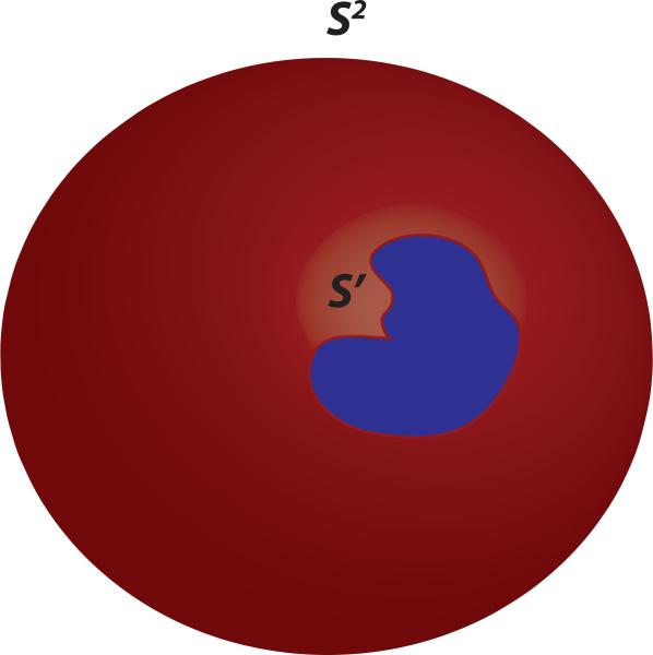
Note that the 3D MIDAS is finite, so it will not map onto the entire surface of the 4D hypersphere. Rather, the stereographic projection of the MIDAS will lie along a portion of the hyperspherical surface. Consider the illustration in Fig 3. The MIDAS's surface coordinates are mapped onto the region S^′ along the 4D hypersphere. The MIDAS can be interpolated at different (hyperspherical) locations that reside within region S′; using hyperspherical points outside of S′ will result in extrapolation. Therefore, we only use the samples in hysph mesh interp that coincide with S′ in Fig. 3.

Figure 3. HyperSPHARM Interpolation.

In this 3D illustration, a 2D object is stereographically projected onto the 3D sphere S². Since the object is finite, its projection will not occupy the entire surface of the sphere; rather, it will lie along a portion of the spherical surface, which in our illustration is denoted as S′. Points residing within S′ can be used for interpolation, whereas outside points will lead to extrapolation.

4. Data Processing

4.1. Dataset

The dataset used in this study was part of a national study (Midlife in US; http://midus.wisc.edu) for the health and well-being in the aged population (Van Reekum et al., 2011). It comprised 68 healthy adults (22 men; 46 women) ranging in age between 38 to 79 years (mean age = 58.0 ± 11.4 years).

High-resolution T1-weighted inverse recovery fast gradient echo MRI images were obtained using a 3T GE SIGNA scanner with a quadrature head RF coil. A 3D, spoiled gradient-echo (SPGR) pulse sequence was used to generate T1-weighted images. 124 contiguous 1.2-mm axial slices were acquired (TE=1.8 ms; TR=8.9 ms; flip angle = 10°; FOV = 240 mm; 256 × 256 data acquisition matrix).

4.2. Establishment of Correspondence

Correspondence for SPHARM and HyperSPHARM was established in a similar manner as proposed in (Chung et al., 2007). Brain tissues in the MRI scans were automatically extracted using Brain Extraction Tool (BET) (Smith, 2002) and trained raters manually segmented the amygdalae and hippocampi, which form our MIDAS. A nonlinear image registration using the diffeomorphic shape and intensity averaging technique with the cross-correlation as the similarity metric through Advanced Normalization Tools (ANTS) (Avants et al., 2008) was performed on the T1-weighted images, and a study-specific template was constructed from a random subsample of ten subjects. The deformation field is then used to warp any individual brain to the template. Specifically, we deformed the amygdala and hippocampus binary masks to the template space. The normalized masks were then averaged to produce the subcortical masks. The iso-surfaces of the subcortical masks were then extracted using the marching cube algorithm (Lorensen and Cline, 1987). The number of mesh vertices for each cortical structure are as follows: 1296 for left amygdala, 1324 for right amygdala, 2444 for left hippocampus, and 2554 for right hippocampus. Hence, the MIDAS comprises 7618 mesh vertices.

Using ANTS, we obtained the deformation vector field, which is defined on voxels, that warps an individual brain to the template. On the other hand, the vertices of the subcortical surfaces meshes are located within the voxels, so we simply assigned the vector field onto the mesh vertices by linear interpolation.

Please note that SPHARM and HyperSPHARM were not directly used to establish correspondence for this dataset. As mentioned, ANTS was used to align and establish non-linear correspondence, so vertex-to-vertex correspondence was present before application of HyperSPHARM/SPHARM. However, SPHARM and HyperSPHARM further register the surfaces post-alignment via surface flattening and stereographic projection, respectively. Hence, our approach avoids the surface alignment done by coinciding the first order ellipsoid meridian and equator in the SPHARM-correspondence approach (Gerig et al., 2001; Styner et al., 2006). Surface meshes obtained from other segmentation techniques such as FreeSurfer (Fischl and Dale, 2000) may require the SPHARM-correspondence approach.

4.3. SPHARM Processing

HyperSPHARM is compared to the widely used SPHARM framework. SPHARM processing somewhat differs from that of HyperSPHARM, so we will now elaborate on it. SPHARM has to be applied to each individual structure forming the MIDAS. Thus, for a SPHARM representation of order L, a total of 3(L + 1)² expansion coefficients parameterize a single structure and 12(L+1)² coefficients all four disconnected structures (i.e. left and right hippocampus and amygdala). First, each cortical structure is mapped onto a unit sphere using diffusion mapping (Chung et al., 2010), where the number of vertices of the spherical mesh is equal to that of the cortical mesh. We denote this spherical mesh as sph mesh interp. The spherical mesh is then refined by resampling to a uniform grid along the sphere, whose number of vertices totals 40962. SPHARM is then performed using this refined spherical mesh, and MSE_SPHARM denotes the mean squared error between the SPHARM reconstruction and refined spherical mesh. The SPHARM coefficients are then used to interpolate the cortical surface coordinates using the spherical mesh sph mesh interp, and × denotes the mean squared error between the SPHARM-interpolated values and the mesh sph mesh interp. This analysis is repeated for each cortical structure forming the MIDAS. Please note that the translation of the surface coordinates closer to the origin is also employed for SPHARM.

4.4. Selection of Optimal p_o

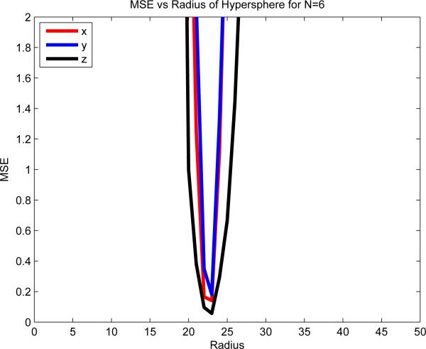
Choosing the optimal hypersphere radius p_o for HyperSPHARM reconstruction may be determined by plotting the ${\mathrm{MSE}}_{\mathrm{HSH}}^{\mathrm{interp}}$ versus p_o for the MIDAS reconstruction. Note the analysis is done on the mean population template instead of each individual subject so to minimize inter-subject variability. The HSH of truncation order N = 6 are used for the HyperSPHARM reconstruction of the template. Lower truncation orders were found to interpolate poorly, so are excluded from the analysis. Fig. 4 displays the plot of the ${\mathrm{MSE}}_{\mathrm{HSH}}^{\mathrm{interp}}$ of each vⁱ as a function of p_o, and indicates that ${\mathrm{MSE}}_{\mathrm{HSH}}^{\mathrm{interp}}$ is minimized at p_o = 23, which we adopt as our radius.

Figure 4.

Plot of ${\mathrm{MSE}}_{\mathrm{HSH}}^{\mathrm{interp}}$ as a function of the hypersphere radius p_o. The HyperSPHARM coefficients are estimated using the population template, and then used to interpolate along the hyperspherical mesh hysph mesh interp. The HSH of truncation order N = 6 are employed. The MSE is minimized at p_o = 23, which we adopt as our radius.

Table 2 displays the optimal radius for different truncation orders of HyperSPHARM reconstruction. The optimal radius is more or less the same across N.

Table 2.

Optimal Radius for a Given Truncation Order N

N	W	Optimal po	${\mathrm{MSE}}_{\mathrm{HSH}}^{\mathrm{interp}}$
2	14	24	5.08
4	55	23	0.424
6	140	23	0.413

5. Experiments and Results

5.1. Rotational Variance of HyperSPHARM

The rotational variance of stenographic projection depends on the nature of an object's symmetry. Axially symmetric objects will be rotationally invariant over the projection. However, non-axially symmetric objects, such as the limbic structures, will be rotationally variant over the mapping. Hence, the rotation of the MIDAS will affect the subsequent HyperSPHARM reconstruction.

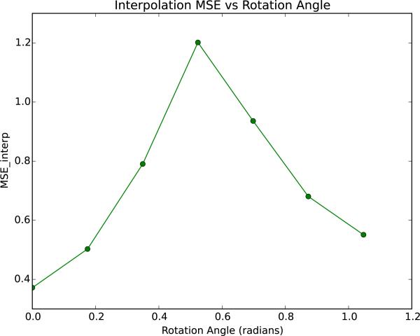
Fig. 6 displays the plot of the ${\mathrm{MSE}}_{\mathrm{HSH}}^{\mathrm{interp}}$ of the population template as a function of the rotation angle. The graph is approximately concave down, and the ${\mathrm{MSE}}_{\mathrm{HSH}}^{\mathrm{interp}}$ peaks at 30°.

Figure 6.

We rotate the MIDAS by some angle to see how the subsequent HyperSPHARM reconstruction is affected. Plot of ${\mathrm{MSE}}_{\mathrm{HSH}}^{\mathrm{interp}}$ as a function of the rotation angle is shown above. The HyperSPHARM coefficients are estimated using the population template, and then used to interpolate along the hyperspherical mesh hysph mesh interp. HyperSPHARM parameters are N = 6 and p_o = 23. The plot confirms the rotational variance of HyperSPHARM, which is due to stereographic projection being dependent on rotation.

5.2. Simulation Study

We have performed two simulation studies to determine if HyperSPHARM can characterize general shape differences between two distinct populations. Hotelling T² test and support vector machines are used to assess Hyper-SPHARM's effectiveness. HyperSPHARM parameters are N = 6 and p_o = 23, which results in W = 140 expansion coefficients for each surface coordinate, while L = 20 SPHARM representation is employed.

Voxel-wise Hotelling T-Squared Test

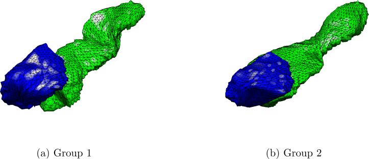
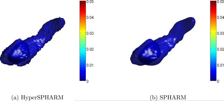
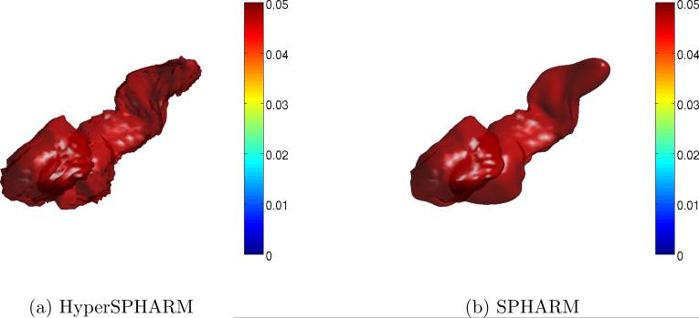
In the first simulation experiment, we formed two distinct groups by selecting the right amygdala and right hippocampus of subjects 10 and 68. As can be seen in Fig. 7, there are obvious shape differences between the two subject's limbic structures. We simulated 30 versions of each group by adding Gaussian noise N(0, 0.01) to each group's surface, thereby creating two distinct populations. Hyper-SPHARM and SPHARM are then used to reconstruct the surfaces. We test for group differences by carrying out the Hotelling T² test at the voxel level on the HyperSPHARM/SPHARM-parameterized surfaces. The resulting p-values were corrected for multiple comparisons across all vertices using false discovery rate (FDR) (Benjamini and Hochberg, 1995), and are projected onto the average of the 60 simulated surfaces for each method (Fig. 8). We detect group differences using each method, with all voxels being statistically significant (p-value< 1e − 10), which is what we expect given the manifest shape differences between the two populations.

Figure 7. Simulation Experiment I.

We select the right hippocampus and right amygdala of two subjects that exhibit manifest shape differences, and create two distinct groups by adding Gaussian noise N(0, 0.01) to each subject's surface.

Figure 8. Simulation Experiment I Results.

We carry out a Hotelling T² test to see if HyperSPHARM/SPHARM can distinguish between two groups that have manifest shape differences. The p-values after FDR correction (i.e. q-value) are projected back onto the template, which is the average of the 60 simulated surfaces. Group differences are detected using each method, with all voxels statistically significant.

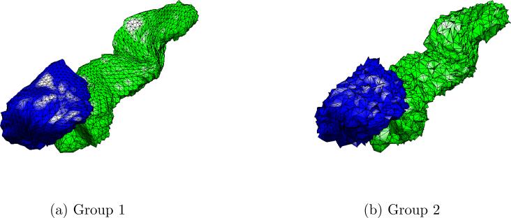
In the second simulation experiment, we looked at two distinct groups that barely have any shape differences. We selected the right hippocampus and right amygdala of subject 10. The first group was formed by simulating 30 versions of subject 10's right limbic structures by adding Gaussian noise N(0, 0.01) to the surface. The second group was formed by simulating 30 versions using Gaussian noise N(0, 0.16). Fig. 9 displays a member of each group. HyperSPHARM and SPHARM are then used to reconstruct the surfaces. We test for group differences by carrying out the Hotelling T² test at the voxel level on the HyperSPHARM/SPHARM-parameterized surfaces. The resulting p-values were corrected for multiple comparisons across all vertices using FDR, and are projected onto the average of the 60 simulated surfaces for each method (Fig. 10). No group differences are detected using each method, with all voxels being statistically insignificant (p-value= 1), so indicating that both methods will not distinguish between two groups that are nearly identical in shape.

Figure 9. Simulation Experiment II.

We select the right hippocampus and right amygdala of a subject. We create two distinct groups that barely have any shape differences. The first group was formed by adding Gaussian noise N(0, 0.01) to the surface, while the second was created using N(0, 0.16).

Figure 10. Simulation Experiment II Results.

We carry out a Hotelling T² test to see if HyperSPHARM/SPHARM can distinguish between two groups that are nearly identical in shape. The p-values after FDR correction (i.e. q-value) are projected back onto the template, which is the average of the 60 simulated surfaces. No group differences are detected using each method, with all voxels statistically insignificant.

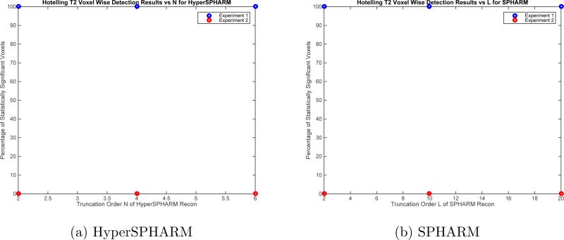
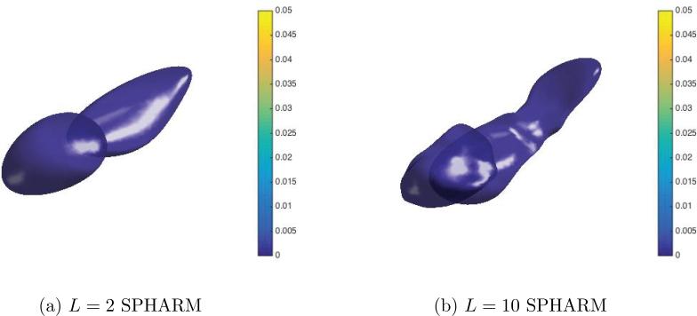
Fig. 11 plots the number of statistically significant voxels obtained by HyperSPHARM/SPHARM for each simulation experiments as a function of the truncation order, indicating that the same detection results can be achieved using lower order HyperSPHARM/SPHARM expansions. It should be noted that L = 2 SPHARM reconstruction greatly over-smoothens the MIDAS, as shown in Fig. 12, while L = 10 moderately over-smoothens. For this reason, we feel L = 20 is the most appropriate truncation order for SPHARM.

Figure 11.

Plot of the percentage of statistically significant voxels as a function of truncation order for each simulation experiments using Hyper-SPHARM and SPHARM. Experiment I involves Hotelling T² analysis of two distinct groups characterized by major shape differences between them, while Experiment II looks at two distinct groups characterized by very little shape differences between them.

Figure 12.

The SPHARM results for Simulation Experiment I using L = 2 and L = 10. Although consistent with L = 20 SPHARM results, the lower-order SPHARM representations over-smooth the MIDAS, especially L = 2.

These two experiments demonstrate that HyperSPHARM is capable of detecting sufficiently large shape differences, and further demonstrate that what HyperSPHARM detected in the real data is of a sufficiently large shape difference. Otherwise, it would not have the detected group-wise differences in the first place.

Support Vector Machines

For each simulation experiment, we also employed the HyperSPHARM coefficients as features of object classification using linear support vector machines (SVM). Linear SVM (Cortes and Vapnik, 1995) seek an optimally separating hyperplane to distinguish between two classes within a feature space. In our situation, the shape invariants (i.e. HyperSPHARM and SPHARM coefficients) form the feature space. Likewise, the binary classes in each experiment are the two distinct groups. We used MAT LAB Statistics T oolbox (MATLAB, 2013) to perform the SVM analysis.

Each surface is characterized by 420 HyperSPHARM features and 2646 SPHARM features. The number of features for each method is too large to train a good model given our total number of surfaces, i.e. 60. Feature selection is needed.

Following (Shen et al., 2004), we test the effectiveness of the features by employing a simple two-sample t-test on each feature. We obtain a p-value associated with the test statistic

$$T=\frac{{\overline{Y}}_1-{\overline{Y}}_2}{\sqrt{s_1^2∕N_1+s_2^2∕N_2}},$$ (9)

where N₁ and N₂ are the sample sizes, ${\overline{Y}}_1$ and ${\overline{Y}}_2$ are the sample means, $s_1^2$ and $s_2^2$ are the sample variances, and the samples are the values of each feature across all subjects in the two respective classes. A lower p-value implies stronger group differences statistically and corresponds to a more significant feature.

We performed a leave-one-out test for each simulated surface, where we selected the first n features ordered by p-value associated with t-test applied to each leave-one-out training set separately. Hence, different leave-one-out tests may have different numbers of significant features. For an impartial comparison between SPHARM and HyperSPHARM, we make sure the number of significant features expended by each method is approximately the same. In the first simulation experiment, the outputting of 1-2 significant features for each leave-one-out test by feature selection yielded a 100 % classification accuracy for both SPHARM and HyperSPHARM. Likewise, the outputting of 40-44 significant features for each leave-one-out test also resulted in a 100 % classification accuracy for both methods. In the second simulation experiment, no significant features were yielded for either method.

The linear SVM results are consistent to those of the Hotelling T² test, and these two differing analyses demonstrate that both the HyperSPHARM-parameterized surface coordinates and HyperSPHARM coefficients are able to distinguish between two groups that exhibit sufficiently large shape differences. Most importantly, according to both the Hotelling T² and SVM results, HyperSPHARM's performance is comparable to SPHARM in a controlled simulation study.

5.3. HyperSPHARM Reconstructions and Comparison to SPHARM

HyperSPHARM was used to reconstruct the MIDAS comprising the left and right hippocampus and amygdala for 68 subjects. For the entire MIDAS, the HyperSPHARM parameters were radius p_o = 23 and N = 6, which results in W = 140 HSH expansion coefficients for each sⁱ. So a total of 420 HSH coefficients parameterize the entire MIDAS. SPHARM has to be applied to each individual structure forming the MIDAS. The L = 20 SPHARM representation was used, which results in 1323 SPHARM coefficients parameterizing each cortical structure and 5292 parameterizing the entire MIDAS.

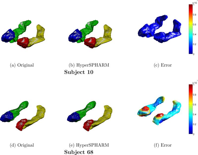
Fig. 5 shows the HyperSPHARM-reconstructed surfaces for two different subjects. The length of the residual is also computed and plotted on the reconstructed surfaces. The MSE_HSH for the first subject is on the order of 10⁻⁶ while that of the second subject is 10⁻².

Figure 5.

HyperSPHARM (N = 6) representations of amygdala and hippocampus surfaces for subjects 10 and 68. The vertex-wise reconstruction errors are also plotted.

Tables 3 and 4 display the reconstruction errors of SPHARM and HyperSPHARM representations, respectively. According to the two tables, MSE_SPHARM < MSE_HSH for the amygdalae, which is not surprising since SPHARM performs very well on approximately spherical objects. However, MSE_SPHARM > MSE_HSH for the hippocampi, which significantly deviate from a spherical-like shape. An impartial comparison of the interpolation errors between SPHARM and HyperSPHARM is difficult because a different interpolating mesh was used for each method. However, HyperSPHARM's interpolation error ${\mathrm{MSE}}_{\mathrm{HSH}}^{\mathrm{interp}}$ is reasonably low, and much smaller and less variable than SPHARM's interpolation error in the hippocampi. Hence, we can conclude that HyperSPHARM is appropriate as an interpolating scheme.

Table 3.

SPHARM Mean Squared Error

	MSESPHARM	${\mathrm{MSE}}_{\mathrm{SPHARM}}^{\mathrm{interp}}$
Left Amygdala	0.0843 ± 0.0183	0.0947 ± 0.0195
Right Amygdala	0.0941 ± 0.0165	0.103 ± 0.0171
Left Hippocampus	0.364 ± 0.732	3.91 ± 3.42
Right Hippocampus	0.192 ± 0.314	1.28 ± 4.82

The mean squared error (MSE) and its standard deviation of reconstruction for SPHARM L = 20 reconstruction. MSE is computed over all mesh vertices and averaged over all 68 subjects. Order 20 SPHARM representation expends 21² = 441 basis functions for each surface coordinate of each cortical structure.

Table 4.

HyperSPHARM Mean Squared Error

	MSEHSH	${\mathrm{MSE}}_{\mathrm{HSH}}^{\mathrm{interp}}$
Left Amygdala	0.147 ± 0.609	NA
Right Amygdala	0.148 ± 0.632	NA
Left Hippocampus	0.129 ± 0.511	NA
Right Hippocampus	0.127 ± 0.504	NA
hysph_mesh_interp	NA	0.833 ± 1.09

The mean squared error (MSE) and its standard deviation of reconstruction for HyperSPHARM N = 6 reconstruction. MSE is computed over all mesh vertices and averaged over all 68 subjects. Order 6 HyperSPHARM representation expends 140 basis functions for each surface coordinate of MIDUS. NA stands for ‘Not Applicable’.

5.4. HyperSPHARM as a Data Smoothing Technique: Influence of Age and Gender

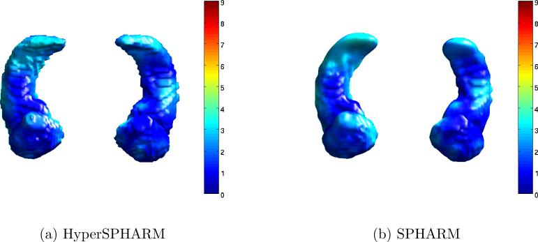
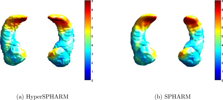
HSH and SPHARM representations were obtained for hippocampus and amygdala surfaces of all 68 subjects. Such representations behave like a surface smoothing technique that removes high frequency noise, as shown in Figure 5. The 69 reconstructed surfaces are then averaged to produce the population specific template. The 3D displacement vector field from the template to individual surface is taken as the response vector in the multivariate general linear model (MGLM) (Chung et al., 2010) and its T -statistic is computed and thresholded at p < 0.05. The random field based multiple comparisons are performed to give stringent results. Neither method detected gender effects on any of the structures (see Fig. 13). However, both methods detected statistically significant age effects, mainly in the tail regions of the hippocampus and small portions of the amygdala (see Fig. 14). The statistical results given by both HyperSPHARM and SPHARM are nearly identical.

Figure 13.

Statistical testing for gender effects in the hippocampi and amygdalae thresholded at p < 0.05 (corrected). A T-statistic exceeding 4.8 indicates statistical significance. No statistically significant gender effect was detected using either method.

Figure 14.

Statistical testing for age effects in the hippocampi and amygdalae thresholded at p < 0.05 (corrected). A T-statistic exceeding 4.8 indicates statistical significance. Statistically significant age effects were detected, mainly in the tail regions of the hippocampi, using both methods.

5.5. Hotelling T² Test on HyperSPHARM Coefficients to Test for Gender Effects

We then carried out the Hotelling T² test on the HyperSPHARM/SPHARM coefficients between each gender to see if any of the coefficients were statistically significant in detecting gender effects. For HyperSPHARM, each subject's coefficient matrix is 140 × 3, whereas for SPHARM each cortical structure of each subject is characterized by a 441 × 3 matrix. Merging each subject's SPHARM coefficients across all four cortical structures results in a 1764 × 3 matrix. The resulting statistical analysis yielded no statistically significant coefficients (corrected for multiple comparison using FDR at 0.01 level) for both SPHARM and HyperSPHARM. Hence, not a single coefficient from either method was found to significantly differentiate between gender. Such a result is consistent with the voxel-wise MGLM analysis, which detected no gender effects in any of the structures.

5.6. Support Vector Machine Classification of Gender

SPHARM parameterization of the hippocampus has been utilized in a support vector machine setting to classify schizophrenia (Shen et al., 2004) and Alzheimer's disease (Gutman et al., 2009). We now assess the ability of the HyperSPHARM coefficients, which form a global shape descriptor of the MIDAS, to classify gender in the hippocampi and amygdalae using linear SVM. For gender, there are 22 males and 46 females.

In order to make an impartial comparison to HyperSPHARM, SPHARM SVM analysis is done on the MIDAS as a whole. Hence, we combine the SPHARM coefficients across all four cortical structures. We define the classification accuracy rate as the probability that a class is correctly identified when each subject is left out once.

Each subject is characterized by 420 HyperSPHARM features and 5292 SPHARM features. The number of features for each method is too large to train a good model given our number of subjects. We employ feature selection in the same manner as done for the simulation experiments.

The yielding of 2-11 statistically significant features for each leave-oneout test by feature selection resulted in a 57 % gender classification accuracy for both HyperSPHARM and SPHARM. Likewise, the outputting of 19-37 significant features for each leave-one-out test yielded a gender classification accuracy of 50 % and 54 % for HyperSPHARM and SPHARM, respectively.

Females make up a little more than 2/3 of the sample size, so 68% can be viewed as the baseline classification accuracy rate. Both HyperSPHARM's and SPHARM's classification accuracies are well below that, indicating that the coefficients are unable to well classify gender based on shape differences in the limbic structures, alone. Such an observation is consistent with the MGLM analysis of the displacement vector field and Hotelling T² test on expansion coefficients, which detected no significant gender effects in the limbic structures.

6. Discussion

The results from the MGLM analysis, Hotelling T² test on expansion coefficients, and SVM classification suggest that gender-driven shape differences in the limbic structures are negligible. However, it could also be that the limbic structures exhibit highly localized shape differences between genders; both HyperSPHARM and SPHARM, being global bases, would be unable to detect such finely-drawn differences. Localization power, which can be obtained via wavelets, is needed to detect subtle shape differences.

Based on our analyses, HyperSPHARM and SPHARM essentially yield the same results. The power of HyperSPHARM, however, lies in its simplicity, versatility, and efficiency. It is simple and fast because it does not require any sort of laborious pre-processing (e.g. surface flattening): mathematically, it is much easier to map a 3D volume onto a 4D sphere than a 3D sphere. HyperSPHARM is versatile because it can handle any geometry, independent of topology, with relative ease. SPHARM, however, is confined to single connected structures. Most significantly, HyperSPHARM possess greater computational efficiency than SPHARM because it expends fewer basis functions in parameterizing multiple disjoint objects.

Studying and quantifying the development of anatomical structures over time is important in medical image analysis. The topology of anatomical structures can change during the course of human growth, as is evidenced by the hyoid bone. At birth, the (human) hyoid bone consists of three disjoint components, but these components will eventually fuse together at around age 40. In other words, before the age of 40 the hyoid bone constitutes a MIDAS, but then develops into a single connected surface. In a developmental study on the hyoid bone then, such longitudinal bone fusion would not be an issue for HyperSPHARM because of its ability to treat multiple disjoint structures as a single entity. SPHARM, however, will initially parameterize three different structures, but eventually only a single structure once the components have fused. Consequently, there will be a disparity in the number of SPHARM coefficients between the two developmental stages (i.e. 3 vs. 1), which poses significant statistical challenges in terms of comparison of the coefficients between the two stages.

Another advantage of HyperSPHARM with regards to developmental studies is illustrated by the following case example: consider a longitudinal study of the hyoid bone that acquires measurements of its bone density over time. The hyoid bone's surface coordinates x, y, and z and bone density constitute 4D data, which can then be stereographically projected onto a 5D hypersphere. Consequently, we will obtain a concurrent mathematical representation of bone density and surface coordinates in terms of the 5D HSH that can be used to examine the hyoid bone's surface evolution in terms of bone density.

7. Conclusion

In this paper, we presented a new analytic approach for representing multiple disconnected shapes using a single parameterization, which is a linear combination of HSH. The method was used to parameterize four disconnected subcortical structures (two amygdalae and two hippocampi), and was found to be more efficient than SPHARM because its parameterization expended fewer basis functions. The resulting HSH coefficients are global and contain information about all four structures as a whole, so they do not provide any local shape information. HyperSPHARM, however, could be adapted to sparse techniques such as wavelets, which will be explored in future. Despite HSH being a global basis, by reconstructing surfaces at each voxel and using HSH as a way to filter out high frequency noise, it was possible to use HyperSPHARM for local inference at vertex level as shown by our application. Although the individual image volumes are registered to a template using diffeomorphic warping (Avants et al., 2008), we might only need an affine registration to initially align the structures and simply match the coefficients as in SPHARM (Chung et al., 2010), but the issue is left as a future study. Additional future work includes investigating whether the HyperSPHARM coefficients (employed in an object classification setting) can boost the power of discrimination for clinical populations.

Research Highlights.

• Introduce HyperSPHARM for simultaneous parameterization of multiple disjoint objects.

• Compare HyperSPHARM to widely used SPHARM in both a controlled simulation study and a real dataset, and will show that HyperSPHARM possesses greater computational efficiency.

• Employ isotropic sampling along 4D sphere for HyperSPHARM interpolation.

• Employ HyperSPHARM representation as a data smoothing technique and HyperSPHARM coefficients for object classification using support vector machines.

Appendix A. Generalized Spherical Harmonics

Consider the d-dimensional unit sphere S^d−1 existing in ${\mathbb{R}}^d$. The eigenfuctions of the Laplace-Beltrami operator on S^d−1 are the d-dimensional spherical harmonics Y_λk...1m(Ω_d−1):

$${\Delta }_{S^{d-1}}{Y}_{\lambda \kappa \dots lm}\left({\Omega }_{d-1}\right)=-l(l+d-2)Y_{\lambda \kappa \dots lm}\left({\Omega }_{d-1}\right),$$

where Ω_d−1 = (η_d−3, . . . , η₁, θ, ϕ) obey (η_d−2 ∈ [0, π], . . . , η₁ [0, π], θ ∈ [0, π], ϕ ∈ [0, 2π]) and are the set of angles defining d-dimensional sphere.

The d-dimensional spherical harmonics are defined as (Aquilanti et al., 1997)

$$Y_{\lambda \kappa \dots lm}\left({\Omega }_{d-1}\right)=2^{\kappa +\frac{d}{2}-2}\left(\kappa +\frac{d}{2}-2\right)!\sqrt{\frac{(2\lambda +d-2)(\lambda -\kappa )!}{\pi (\lambda +\kappa +d-3)!}}{\sin }^{\kappa }\left({\eta }_{d-3}\right)\times C_{\lambda -\kappa }^{\kappa +\frac{d}{2}-1}\left(\cos {\eta }_{d-3}\right)Y_{\kappa \dots lm}\left({\Omega }_{d-2}\right),$$

where Y_k...1m(Ω_d−2) are the (d − 1) spherical harmonics and $C_{\lambda -\kappa }^{\kappa +\frac{d}{2}-1}$ are the Gegenbauer polynomials. The index λ is the grand orbital angular momentum quantum number, and these (d − 1) integers obey the conditions λ = 0, 1, 2, . . . , 0 ≤ k ≤ λ, 0 ≤ l ≤ k, and −l ≤ m ≤ l. When d = 4, $Y_{\lambda \kappa ...lm}\left({\Omega }_{d-1}\right)=Z_{nl}^m(\beta ,\theta ,\varphi )$, i.e. the 4D HSH. The d-dimensional spherical harmonics form an orthonormal basis on S^d−1.

Appendix B. Generalized Stereographic Projection

For centuries, cartographers have struggled with the problem of how to represent the spherical-like surface of the Earth on a flat sheet of paper. One way to achieve this is via stereographic projection. To illustrate it, consider the simpler 3D case. The goal of stereographic projection is to associate each 2D point (u, v) in the equatorial plane with a unique point P = (x, y, z) on the unit sphere. To achieve this, we construct the 3D line that passes through the north pole N = (0, 0, 1) of the sphere and the given point (u, v, 0). This line touches the surface of the sphere at exactly one point, P , so the point P = (x, y, z) is the stereographic projection of the point (u, v).

We will now derive the relationship between the coordinates of a (d − 1)-dimensional Cartesian lattice and those of the sphere S^d−1 based on stereo-graphic projection. The d-dimensional sphere S^d−1 of radius ρ is defined by the coordinates

$$\begin{array}{cc}\hfill u_1=\rho \sin {\eta }_{d-3}\cdots \sin {\eta }_1\sin \theta \cos \varphi & \hfill \\ \hfill u_2=\rho \sin {\eta }_{d-3}\cdots \sin {\eta }_1\sin \theta \sin \varphi & \hfill \\ \hfill u_3=\rho \sin {\eta }_{d-3}\cdots \sin {\eta }_1\cos \theta & \hfill \\ \hfill ⋮& \hfill \\ \hfill u_{d-1}=\rho \sin {\eta }_{d-3}\cos {\eta }_{d-4}& \hfill \\ \hfill u_d=\rho \cos {\eta }_{d-3}& \hfill \end{array}$$

The (d − 1)-dimensional Cartesian lattice is defined by the coordinates x = (x₁, x₂, . . . , x_d−1). The d-dimensional line that passes through the north pole of S^d−1, (0, 0, 0, . . . , ρ), and some point in the Cartesian lattice is parameterized as

$$\begin{array}{cc}\hfill u_1=t{x}_1& \hfill \\ \hfill u_2=t{x}_2& \hfill \\ \hfill u_3=t{x}_3& \hfill \\ \hfill ⋮& \hfill \\ \hfill u_d=\rho (1-t)& \hfill \end{array}$$

where −∞ < t < ∞. The line touches S^d−1 when t satisfies

$$p^2=u_1^2+u_2^2+\cdots +u_d^2=t^2(x_1^2+x_2^2+\cdots +x_{d-1}^2)+{\rho }^2(1-2t+t^2),$$

whose solution is

$$t=\frac{2{\rho }^2}{{\Vert \mathbf{x}\Vert }^2+{\rho }^2}$$

Note that t = 0 is a trivial solution because it corresponds to north pole of S^d−1. Upon substitution, the relationship between the two coordinate spaces is

$$\begin{array}{cc}\hfill u_1=\frac{2{\rho }^2{x}_1}{{\Vert \mathbf{x}\Vert }^2+{\rho }^2}& \hfill \\ \hfill u_2=\frac{2{\rho }^2{x}_2}{{\Vert \mathbf{x}\Vert }^2+{\rho }^2}& \hfill \\ \hfill u_3=\frac{2{\rho }^2{x}_3}{{\Vert \mathbf{x}\Vert }^2+{\rho }^2}& \hfill \\ \hfill ⋮& \hfill \\ \hfill u_d=\frac{\rho ({\Vert \mathbf{x}\Vert }^2+{\rho }^2)}{{\Vert \mathbf{x}\Vert }^2+{\rho }^2}& \hfill \end{array}$$

References

- Angenent S, Hacker S, Tannenbaum A, Kikinis R. On the laplace-beltrami operator and brain surface flattening. IEEE Transactions on Medical Imaging. 1999;18:700–711. doi: 10.1109/42.796283. [DOI] [PubMed] [Google Scholar]
- Aquilanti V, Cavalli S, Coletti C. The d-dimensional hydrogen atom: hyperspherical harmonics as momentum space orbitals and alternative Sturmian basis sets. Chemical Physics. 1997 [Google Scholar]
- Avants B, Epstein C, Grossman M, Gee J. Symmetric diffeomorphic image registration with cross-correlation: Evaluating automated labeling of elderly and neurodegenerative brain. Medical image analysis. 2008;12:26–41. doi: 10.1016/j.media.2007.06.004. [DOI] [PMC free article] [PubMed] [Google Scholar]
- Benjamini Y, Hochberg Y. Controlling the false discovery rate: a practical and powerful approach to multiple testing. Journal of the Royal Statistical Society. 1995;57:289–300. [Google Scholar]
- Bonvallet B, Griffin N, Li J. 3D shape descriptors: 4D hyperspherical harmonics ’An exploration into the fourth dimension’. IASTED International Conference on Graphics and Visualization in Engineering. 2007:113–116. [Google Scholar]
- Brechbuhler C, Gerig G, Kubler O. Parametrization of closed surfaces for 3d shape description. Computer Vision and Image Understanding. 1995;61:154–170. [Google Scholar]
- Chung M, Worsley K, Brendon M, Dalton K, Davidson R. General multivariate linear modeling of surface shapes using SurfStat. NeuroImage. 2010;53:491–505. doi: 10.1016/j.neuroimage.2010.06.032. [DOI] [PMC free article] [PubMed] [Google Scholar]
- Chung MK, Dalton KM, Shen L, Evans AC, Davidson RJ. Weighted Fourier series representation and its application to quantifying the amount of gray matter. IEEE Transac. Med. Imaging. 2007;26:566–581. doi: 10.1109/TMI.2007.892519. [DOI] [PubMed] [Google Scholar]
- Cortes C, Vapnik V. Support-vector networks. Mach Learn. 1995;20:273–297. [Google Scholar]
- Domokos G. Four-dimensional symmetry. Physical Review. 1967;159:1387– 1403. [Google Scholar]
- Fischl B, Dale AM. Measuring the thickness of the human cerebral cortex from magnetic resonance imagings. PNAS. 2000;97:11050–11055. doi: 10.1073/pnas.200033797. [DOI] [PMC free article] [PubMed] [Google Scholar]
- Fock V. Zur theorie des wasserstoffatoms. Z. Physik. 1935;98:145–154. [Google Scholar]
- Gerig G, Styner M, Jones D, Weinberger D, Lieberman J. Shape analysis of brain ventricles using spharm. MMBIA. 2001:171–178. [Google Scholar]
- Gu X, Wang Y, Chan T, Thompson T, Yau S. Genus zero surface conformal mapping and its application to brain surface mapping. IEEE Transactions on Medical Imaging. 2004;23:1–10. doi: 10.1109/TMI.2004.831226. [DOI] [PubMed] [Google Scholar]
- Gutman B, Wang Y, Morra J, Toga AW, Thompson PM. Disease classification with hippocampal shape invariants. Hippocampus. 2009;19:572–578. doi: 10.1002/hipo.20627. [DOI] [PMC free article] [PubMed] [Google Scholar]
- Hosseinbor AP, Chung MK, Schaefer SM, van Reekum CM, Peschke-Schmitz L, Sutterer M, Alexander AL, Davidson RJ. 4D hyperspherical harmonic (HyperSPHARM) representation of multiple disconnected brain subcortical structures. MICCAI. 2013:598–605. doi: 10.1007/978-3-642-40811-3_75. [DOI] [PMC free article] [PubMed] [Google Scholar]
- Hurdal MK, Stephenson K. Cortical cartography using the discrete conformal approach of circle packings. NeuroImage. 2004;23:S119–S128. doi: 10.1016/j.neuroimage.2004.07.018. [DOI] [PubMed] [Google Scholar]
- Koay CG. A simple scheme for generating nearly uniform distribution of antipodally symmetric points on the unit sphere. Journal of Computational Science. 2011;2:377–381. doi: 10.1016/j.jocs.2011.06.007. [DOI] [PMC free article] [PubMed] [Google Scholar]
- Koay CG. Distributing points uniformly on the unit sphere under a mirror reflection symmetry constraint. Journal of Computational Science . 2014a [Google Scholar]
- Koay CG. Pseudometrically constrained centroidal voronoi tessellations: Generating uniform antipodally symmetric points on the unit sphere with a novel acceleration strategy and its applications to diffusion and three-dimensional radial MRI. Magn. Reson. Med. 2014b;71:723–734. doi: 10.1002/mrm.24715. [DOI] [PubMed] [Google Scholar]
- Koay CG, Ozarslan E, Basser PJ. A signal transformational framework for breaking the noise floor and its applications in MRI. J. Magn. Reson. 2009;197:108–119. doi: 10.1016/j.jmr.2008.11.015. [DOI] [PMC free article] [PubMed] [Google Scholar]
- Lorensen W, Cline H. Marching cubes: A high resolution 3D surface construction algorithm. Proceedings of the 14th annual conference on Computer graphics and interactive techniques. 1987:163–169. [Google Scholar]
- Mason JK, Schuh CA. Hyperspherical harmonics for the representation of crystallographic texture. 2008;56:6141–6155. [Google Scholar]
- MATLAB . version 8.1.0.604 (R2013a) The MathWorks Inc.; Natick, Massachusetts: 2013. [Google Scholar]
- Shen L, Ford J, Makedon F, Saykin A. Surface-based approach for classification of 3D neuroanatomical structures. Intelligent Data Analysis. 2004;8:519–542. [Google Scholar]
- Smith S. Fast robust automated brain extraction. Human Brain Mapping. 2002;17:143–155. doi: 10.1002/hbm.10062. [DOI] [PMC free article] [PubMed] [Google Scholar]
- Styner M, Oguz I, Xu S, Brechbuhler C, Pantazis D, Levitt J, Shenton M, Gerig G. Framework for the statistical shape analysis of brain structures using spharm-pdm. Insight Journal, Special Edition on the Open Science Workshop at MICCAI. 2006 [PMC free article] [PubMed] [Google Scholar]
- Thomson JJ. On the structure of the atom: an investigation of the stability and periods of oscillation of a number of corpuscles arranged at equal intervals around the circumference of a circle; with application of the results to the theory of atomic structure. Philosophical Magazine. 1904;7:237–265. [Google Scholar]
- Timsari B, Leahy R. An optimization method for creating semi-isometric flat maps of the cerebral cortex. The Proceedings of SPIE, Medical Imaging. 2000 [Google Scholar]
- Van Reekum C, Schaefer S, Lapate R, Norris C, Greischar L, Davidson R. Aging is associated with positive responding to neutral information but reduced recovery from negative information. Social Cognitive and Affective Neuroscience. 2011;6:177–185. doi: 10.1093/scan/nsq031. [DOI] [PMC free article] [PubMed] [Google Scholar]