Assessment of the assessment: Evaluation of the model quality estimates in CASP10

Abstract

The article presents an assessment of the ability of the thirty-seven model quality assessment (MQA) methods participating in CASP10 to provide an a priori estimation of the quality of structural models, and of the 67 tertiary structure prediction groups to provide confidence estimates for their predicted coordinates. The assessment of MQA predictors is based on the methods used in previous CASPs, such as correlation between the predicted and observed quality of the models (both at the global and local levels), accuracy of methods in distinguishing between good and bad models as well as good and bad regions within them, and ability to identify the best models in the decoy sets. Several numerical evaluations were used in our analysis for the first time, such as comparison of global and local quality predictors with reference (baseline) predictors and a ROC analysis of the predictors' ability to differentiate between the well and poorly modeled regions. For the evaluation of the reliability of self-assessment of the coordinate errors, we used the correlation between the predicted and observed deviations of the coordinates and a ROC analysis of correctly identified errors in the models. A modified two-stage procedure for testing MQA methods in CASP10 whereby a small number of models spanning the whole range of model accuracy was released first followed by the release of a larger number of models of more uniform quality, allowed a more thorough analysis of abilities and inabilities of different types of methods. Clustering methods were shown to have an advantage over the single- and quasi-single- model methods on the larger datasets. At the same time, the evaluation revealed that the size of the dataset has smaller influence on the global quality assessment scores (for both clustering and nonclustering methods), than its diversity. Narrowing the quality range of the assessed models caused significant decrease in accuracy of ranking for global quality predictors but essentially did not change the results for local predictors. Self-assessment error estimates submitted by the majority of groups were poor overall, with two research groups showing significantly better results than the remaining ones.

Introduction

Protein models have proven instrumental in addressing various problems of life sciences.^1–3 In the latest two decades many protein structure prediction methods have been developed⁴ and the field of protein structure prediction has evolved⁵ to the point where models can be generated by a nonspecialist with just a few clicks of a computer mouse or simply downloaded from the openly accessible Internet repositories.^6–8 This simplicity, though, bears the risk of misusing the models, as they can span a broad range of the accuracy spectrum and may not be suitable for specific biomedical applications.^9,10

To help navigating the vast numbers of already available models, the computational biology community is paying increasing attention to the a priori model quality prediction problem. The global quality score of a model (ranging from 0 to 1) was introduced to allow a quick grasp of the overall usefulness of the model. At the same time, two models may have the same global score but different accuracy in different regions. Thus, having the right perception of model quality at the residue level is imperative for the end user, for example, interested in the putative binding sites. The assessment of the absolute quality of models on the global and local level is conceptually connected with the problem of model ranking. Hundreds of models may be available for the same amino acid sequence, and it is important to differentiate them.

Within the scope of CASP, the model quality assessments were introduced in 2006 and met with a considerable enthusiasm of the community.^10–12 CASP10 reconfirmed substantial interest in the problem, with 37 groups (including 25 servers) submitting predictions of the global quality of models, 19 - providing estimates of model reliability on a per-residue basis, and 67 - submitting confidence estimates for their own tertiary structure coordinates.

The article summarizes performance of these groups, discusses progress, and identifies remaining challenges in the field.

Materials and Methods

Changes to the testing procedure

The procedure for testing QA prediction methods in CASP10 differed substantially from that of previous CASPs. The changes were implemented to allow a more thorough analysis of the effectiveness of QA methods, and specifically to check two hypotheses discussed in our CASP9 assessment paper.¹⁰ First, we asserted that the observation that single- and quasi-single- model methods are not competitive with clustering methods in model ranking might be related to the large size of the test set that favors clustering approaches. Second, we hypothesized that CASP9 correlation scores are biased (over-inflated), because CASP datasets are more diverse (and therefore easier to assess by predictors) than those that one might expect in real life applications. In particular, we suggested that the outstanding performance of clustering methods in CASP9 (correlation coefficients of over 0.9) could be due to the latter phenomenon. Our hypotheses were based on an a posteriori analysis of the dependence of the assessment scores on the size and diversity of the datasets¹⁰. To enable rigorous analysis of this dependence, we had to ensure that predictors only had access to those models used in the subsequent evaluation. With this in mind, we modified the procedure by releasing models in two stages: first, a small number of models spanning the whole range of model accuracy, and then, a larger number of models of more uniform quality.

Test sets, timeline, and submission stages

The test sets for assessment of the QA methods in CASP10 were prepared as follows. After all the server TS models for a target were collected, we checked them for errors with MolProbity¹³ and ProSA,¹⁴ and structurally compared with each other using LGA¹⁵. All models were then hierarchically clustered into 20 groups based on their pair-wise RMSD and, independently of clustering, ranked according to a reference quality assessment predictor (see description further in Materials). The clustering results along with the model quality checks^13,14 were used to select a subset of 20 models of different accuracy for the first stage of the QA experiment - S20 (stage_1) dataset. In addition, the best 150 models according to the reference consensus QA predictor were selected for the second stage test set – B150 (stage_2).

Stage_1 models were automatically sent to the registered QA servers and released to the regular-deadline QA predictors through the CASP website two days after closing the server structure prediction window for the target. All QA predictors (both servers and regular groups) had two calendar days to submit quality estimates for stage_1 models as QA model_1. After having collected QA predictions for the first stage, we have released the stage_2 test set. All the predictors again had two calendar days to submit quality estimates for the stage_2 models as QA model_2.

For a better understanding of the CASP10 model release procedure, a detailed example of the timeline is provided at http://predictioncenter.org/casp10/index.cgi?page=format#QA.

Prediction formats

In both stages of the experiment, predictors could submit estimates of the overall reliability of models (QA1) and their per-residue accuracy (QA2). For QA1, predictors were asked to score each model on a scale from 0 to 1, with higher values corresponding to better models and the value of 1.0 corresponding to a model virtually identical to the native structure. For the assessment of local accuracy (QA2), predictors were asked to report estimated distances in Ångströms between the corresponding residues in the model and target structures after optimal superposition.

CASP also requested predictors in the TS category to label residues with error estimates in place of the temperature factor field of the conventional PDB format (QA3). This testing mode is conceptually identical to QA2 and differs only in that QA2 predictors work with the broader dataset of server models, while QA3 predictors provide error estimates for their own predictions.

Details of the submission formats are provided at the Prediction Center web page http://predictioncenter.org/casp10/index.cgi?page=format.

Reference consensus methods: Davis-QAconsensusALL and Davis-QAconsensus

A reference consensus quality predictor assigns quality score to a TS model based on the average pair-wise similarity of the model to other models. We developed two reference consensus predictors for CASP10: Davis-QAconsensusALL and Davis-QAconsensus. The two methods are conceptually identical, but operate on different datasets: Davis-QAconsensusALL uses all server models submitted on a target (ca. 300 models per target), while Davis-QAconsensus uses the restricted datasets (B150 or S20). For each TS model, the quality score is calculated by averaging the GDT_TS scores from all pairwise comparisons followed by the normalization of the result by the ratio between the number of residues in the model and in the target.

Targets

In the MQA category, all predictors were asked to submit their quality estimates for all targets, including “all-group” targets (a.k.a. “human/server” targets) and server-only ones. One hundred and fourteen targets were released in CASP10. Seventeen of these were cancelled by the organizers¹⁶ and were also excluded from the QA assessment^*. Additionally, we canceled two more targets as inappropriate for the QA analysis: T0677, for which coordinates were available only for two disjoint domains without a common coordinate system; and T0686, which contained a nonglobular domain oriented differently with respect to the globular part of the protein, in the two different chains present in the unit cell. The remaining 95 targets were assessed.

QA1 and QA2 evaluations are performed at the target level, differently from the TS or QA3 evaluations, which are domain-based.

Predictions

7679 QA predictions for 114 targets were submitted during CASP10; all are accessible at the http://prediction-center.org/download_area/CASP10/predictions/ page (file names starting with QA). 6469 QA predictions on the retained 95 targets were evaluated. These predictions contain quality estimates (global and residue-based) for a subset of 1892 server TS models in stage_1 and 14085 server models in stage_2.

The analyses of model accuracy self-assessments were performed for the groups that submitted at least 10 predictions and had at least two different numerical values in the B-factor field. Following the rules of the tertiary structure assessment, the evaluation was performed at the domain level¹⁶, separately for server groups on all targets (“all group” + “server only”) and for all participating groups on a subset of “all-group” targets. Only the models designated as number 1 were considered. All in all, the QA3 evaluation was run on 3910 server predictions submitted by 35 servers on 122 domains from 95 targets, and 4105 predictions submitted by 67 human-experts and servers on 70 domains from 45 “all-group” targets.

General principles of the evaluation

What is a perfect QA prediction?

Similarly to previous CASPs, we evaluated quality predictions by comparing submitted estimates of global reliability (QA1) and per-residue accuracy (QA2 and QA3) with the values obtained from the LGA¹⁵ superpositions of the models with the corresponding experimental structures (http://predictioncenter.org/download_area/CASP10/results_LGA_sda). In this assessment we postulated that a perfectly predicted QA1 score should correspond to the model's GDT_TS score (divided by 100) and perfectly predicted residue errors (in QA2 and QA3 modes) should reproduce distances between the corresponding residues in the optimally superimposed model and experimental structures.

Per-target vs all models pooled together evaluations

Estimated and observed data can be compared on a target-by-target basis or by pooling models from all targets together.

As an example of the difference between the two approaches, let us consider a dataset consisting of two targets of different difficulty with 3 models submitted for each. Let the observed GDT_TS scores for the models on the harder target be 45, 50, and 55, and on the easier one - 85, 90, and 95. A QA predictor submitting QA1 scores of 65, 70, 75 for both of the targets will achieve a per-target correlation of 1, demonstrating a perfect ability to predict the relative quality of models for each target separately. At the same time, if we pool models from the two targets into a single dataset, the correlation coefficient for this method would only be 0.2, revealing that the method does not discriminate between the relatively poor models for the first target and the good models for the second one.

Thus, the two assessment approaches show different qualities of the methods and we use both of them in this article.

Evaluation measures

The majority of the evaluation measures and assessment procedures that we use in this paper have already been used in the previous CASP assessments. These include:

• correlation of the predicted model accuracy with the observed GDT_TS values (QA1);

• comparative analysis of correlation coefficients for the MQA predictors and the reference consensus predictor (QA1, QA2);

• descriptive statistics and ROC analysis of the ability to discriminate between good and bad models (QA1);

• loss in quality between the best available and the estimated best model, related to the capability of selecting the very best model in a decoy set (QA1);

• correlation between the estimated and actual per-residue distances in the model and the experimental structure (QA2, QA3);

• descriptive statistics measures (Matthews's correlation coefficient) to evaluate the accuracy in identifying reliable and unreliable model regions (QA2);

• ROC analysis of the ability to assign realistic per-residue error estimates for the predictors' own models (QA3);

• comparative analysis of the accuracy of self-assessment quality estimates (QA3) and the results of two reference local quality assessment methods (ProQ2¹⁷ and QMEAN¹⁸ ran with the default parameters).

All these measures and the specifics of their application for evaluation and ranking were comprehensively discussed in our CASP9 assessment papers^10,19. Below we provide a detailed description only for the measures used in this round of CASP for the first time.

Comparing results of local accuracy predictors to those of reference consensus predictors (QA2)

Reference consensus predictors build their scores based on the results of pairwise superpositions of models in the test set. Structural superposition programs (LGA in our case) rotate and translate model coordinates to optimize a structural fit function. From the superimposed coordinates one can assign an error estimate for residue i in the model a as the average of all pairwise distances for this residue using the following formula^20–22:

$$S_i^a=\frac{1}{M-1}\sum _{b\ne a}^M\frac{1}{1+{\left(\frac{d_i^{ab}}{d_0}\right)}^2},$$ (1)

Where $d_i^{ab}$ is the distance between Cα atoms of the corresponding i-th residues in the models a and b, d₀ is a distance threshold regulating the rate of the fall-off of the S-function (here d₀=5) and M is the number of models in the dataset. These dimensionless error values range from 0 to 1 by definition and can be directly used in the ROC calculations (see below) or converted back to the distances $d_i^a$ inversing the formula for the S-function (1).

ROC analysis of the ability to discriminate between reliable and unreliable regions in models (QA2)

In CASP9, we evaluated the ability of predictors to discriminate between well- and poorly modeled residues with Matthews' correlation coefficient.¹⁰ Here we complement this evaluation with a more general analysis based on the ROC technique.

An error estimate is considered correct if the corresponding residues in the optimal structural superposition (LGA) of the model and experimental structure are not further than the specified cutoff (3.8Å). Confidence estimates are converted to the (0;1) range using the S-score like equation (1) and the correspondence between the true and false positive rates of all the QA2 predictors is plotted for different predictive thresholds. The area under the curve (AUC) is used as a measure of the accuracy.

Results and Discussion

As different number of groups participated in prediction of the overall and local accuracy of models, we evaluated performance of the methods in these prediction sub-categories separately. Global quality predictors (QA1) were assessed from three perspectives: ability to (i) provide correct absolute and relative quality annotations for models, (ii) identify the best models in the datasets, and (iii) separate good from bad models. Local quality predictors (QA2 and QA3) were evaluated for their ability to assign accurate error estimates to the modeled residues and discriminate between well and badly modeled regions.

Ability to provide correct model quality estimates

This aspect of quality assessment was evaluated by computing the correlation between the predicted and observed model quality (Fig. 1). The new two-stage QA testing procedure allowed assessing performance on two different datasets of models in two assessment modes (see Materials). Results of the correlation analysis are presented in Figure 1. For each participating group, panels A and B show the average z-score and the weighted mean of the Pearson correlation coefficients calculated for each target on the B150 and S20 datasets, respectively; panels C and D report the Pearson correlation coefficient and the z-score computed on the datasets comprised of all per-target B150 and S20 models, respectively.

Figure 1.

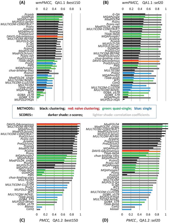
Correlation coefficients for the 37 participating groups and the reference Davis-QAconsensus benchmarking method in per-target based assessment (A, B) and all targets pooled together assessment (C, D). Panels (A) and (C) illustrate the results for the B150 datasets; panels (B) and (D) those for the S20 datasets. Bars showing z-scores are drawn in darker colors; correlation coefficients in lighter colors. The z-scores for the reference method are calculated from the average and standard deviation values of the correlation coefficients for the 37 participating predictors. Clustering methods are shown in black, single model methods in blue, quasi-single model methods in green, and the reference method in red.

In the per-target assessment mode (QA1.1 - panels A and B), the best performing QA predictors reached the wmPMCC close to 0.6 on the B150 datasets and close to 0.9 on the S20 datasets. In the “all models pooled together” mode (QA1.2 – panels C and D), the best methods reach correlation coefficients of around 0.9 on both datasets. Visual inspection of the graphs suggests that the top performing groups obtained very similar results. This observation is confirmed by the results of the statistical significance tests on the common set of predicted targets. According to the paired Student's t-test, the top-ranked twelve predictors in the QA1.1 mode (panels A and B) are indistinguishable from one another at the 0.01 significance level, with the exception of only 5 out of the 132 pairwise comparisons in the two top-12 group sets (see Table S1 in Supporting Information for details). In the QA1.2 mode, the difference between the 1st and the 12th-ranked method is just 0.01 (panel C) and 0.05 (panel D) correlation units. Detailed results of the Z-test comparisons for the top 12 groups on QA1.2 datasets are provided in Table S2 (panel A) of the Supporting Information.

The very similar results of the top-ranked methods may indicate that all top methods are based on a very similar methodology. Indeed, the vast majority of top performing methods in CASP10 use similar approaches based on the consensus of models in the dataset. The dominance of clustering/consensus methods can be easily seen from Figure 1, where black bars (consensus methods) cluster in the upper part of the graphs, while blue bars (single-model methods) are at the bottom of the chart (for a classification and a brief description of CASP10 QA methods please refer to Table I). At the same time, it can be noticed that, for the first time in the last four CASPs, the top part of the correlation analysis tables also contains methods that are not purely clustering in nature. In particular, quasi-single model methods GOAPQA and MQAPsingle appear to be competitive with pure clustering methods on the B150 datasets (panel A), and MQAPsingle, ModFOLD4_single and TSlab-tbQA methods place in the upper part of the tables on the S20 sets (panels B and D). This phenomenon, however, cannot be attributed to a breakthrough in the development of single- and quasi-single- model methods since the CASP10 datasets were intentionally built for being more challenging for clustering methods.

Table I. Classification and Short Description of CASP10 QA Methods.

Method	C/S M	G/L	Scoring function
Ariadne	CM	G	Structural comparison of all models to a set of putatively good models selected with Pcons, ProQ2, PconsD and dDFIRE with subsequent averaging of TM scores and discarding 20% of outliers.
BITS	S/S*	G	Structural quality of predicted binding sites; if no binding site is identified - global structural comparison with a model predicted using multiple templates; if no templates - scoring with a knowledge-based potential.
ConQ	CM	G	Original model ranking with Pcons, ProQ2, PconsD and dDFIRE with subsequent rank adjustment based on predicted contact maps (DCA and PSICOV) and score normalization.
DAVIS-QAconsensus	C	L/G	Average GDT-TS score to all other models in a decoy set with subsequent target length normalization.
GOAPQA	S*	G	A statistical potential – GOAP23, with normalization based on average TM-similarity of a model to the top five GOAP-ranked models.
GOBA_579, GOBA_y579	S*	G	GO-based functional similarity of a model to its structural neighbors with subsequent normalization using ROC analysis.
G-QA	C	G	Average pair-wise similarity of models in the extended dataset complemented with I-TASSER models.
Keasar	S	G	Energy minimization based on secondary structure assignments from PSIPRED and SAM-T08.
ModFOLD422,24	C	L/G	25 Clustering of models in CASP datasets together with IntFOLD2 models using ModFOLDclust2 approach.
ModFOLD4_single	S*	L/G	Comparing every model in the CASP dataset against the pool of IntFOLD2 models using a global and local scoring approach similar to that used by ModFOLDclust2.
ModFOLDclust2 26	C	L/G	Global: mean of the QA scores obtained from the ModFOLDclustQ method and the original ModFOLDclust method; local: the per-residue score taken from ModFOLDclust.
MQAPmulti, MQAPmulti2	C	L/G	Combination of statistical and agreement potentials with pair-wise model comparisons.
MQAPsingle, MQAPsingle2	S*M	L/G	Compares models in the test set against models generated by GeneSilico metaserver using the MQAPmulti(2) algorithm.
MUFOLD-HQA	C	G	A hybrid quality assessment algorithm combining knowledge-based scoring functions and consensus approaches.
MUFOLD-QA27	C	G	Average pair-wise similarity of the model to all models in a test set with complement of models generated by MUFOLD server.
MUFOLD-server	C	G	Combination of single scoring functions (secondary structure, solvent accessibility, torsion angles) with consensus GDT.
MULTICOM-construct	C	L/G	Combination of a single-model score from ModelEvaluator and the weighted average pairwise GDT-TS scores for the model.
MULTICOM-cluster	S	L/G	An SVM-based score combining predicted secondary structure, solvent accessibility and contact probabilities.
MULTICOM-novel28	S	L/G	The same as in Multicom-cluster, but with amino acid features substituted by features from PSI-BLAST sequence profiles.
MULTICOM-refine	C	L/G	Global: pairwise model comparison approach APOLLO; local: average of absolute differences between each residue in the model and the corresponding residues in the set of top models from global QA
Pcomb, Pcons(group)21,29	C	L/G	Combination of structural consensus function Pcons and single model machine learning score ProQ2: 0.8Pcons + 0.2ProQ2
Pcons-net30	CM	L/G	Pure structural consensus (Pcons)
PconsD	C	L/G	Fast, superposition-free method based on consensus of inter-residue distance matrices
PconsQ	C	L/G	Combination of Pcons, ProQ2 and PconsD scoring functions
PMS	S*	G	Similarity to PMS structure models in combination with a single-model score based on random forest approach.
ProQ229,31	S	L/G	Combination of evolutionary information, multiple sequence alignment and structural features of a model using SVM
ProQ2Clust, ProQ2Clust2	C	L/G	Weighted clustering function based on ProQ2 scores
TSlab-psQA	S	G	Difference between distance maps based on multiple sequence alignment complemented with secondary structure and contact prediction.
TSlab-tbQA	S*	G	Combining TSlab-psQA score with template-based evaluation score

(For a more detailed description please consult CASP10 Methods Abstracts - http://predictioncenter.org/casp10/doc/CASP10_Abstracts.pdf). G, a global quality estimator (one score per model); L, a local quality estimator (per-residue reliability scores); S, a single model method capable of generating the quality estimate for a single model without relying on consensus between models or templates; C, a clustering (consensus) method that utilizes information from a provided set of models; S*, a quasi-single model method capable of generating the quality estimate for a single model but only by means of preliminary generation of auxiliary ensembles of models or finding evolutionary related proteins and then measuring similarity of the sought model to the structures in the ensemble; M, a meta-method combining scores from different quality assessment methods.

The rationale for releasing two different datasets in this round was to allow testing of two hypotheses: 1) whether QA methods perform worse on datasets that are still large but more uniform in quality compared to the complete model datasets from previous CASPs and 2) whether clustering methods lose their advantage over nonclustering methods and break down on datasets containing just a few models of different quality. The data in panel A substantiate the first hypothesis, as the average correlation scores for the top performing groups on the B150 datasets is around 0.6, which constitutes a considerable drop from the CASP9 level and is in good agreement with the estimates emerging from Figure 6 of our CASP9 paper¹⁰. The second hypothesis is partially confirmed by the results on the S20 datasets. The data in panel B show that 4 out of 10 top performing methods are quasi-single methods confirming the expectation that nonclustering methods are more competitive with pure clustering methods on sparser datasets. At the same time, very good correlation scores for consensus methods on the S20 sets suggest that these methods in general are able to handle a small number of models and therefore are valuable for ranking models not only within the scope of CASP, where hundreds of models of different quality are available, but also in applications where a much smaller number of diverse models are at hand.

Figure 6.

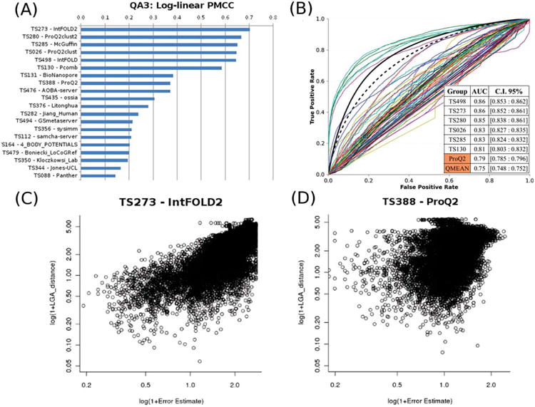
Self-assessment of per-residue model confidence estimates (QA3) on “all-group” targets. (A) Log-linear Pearson correlation coefficients for the top 20 groups. (B) ROC curves for the participating CASP10 methods and two baseline single-model QA methods – ProQ2 and QMEAN. The data for the two baseline methods are plotted as thicker black lines; the QMEAN curve is dashed. The inset shows the AUC scores and 95% confidence intervals for the top eight methods, including the baseline ones. (C, D) Predicted residue errors vs. observed distances for two CASP10 groups: IntFOLD2 (C) and ProQ2 (D).

Comparing the results shown in the four panels of Figure 1, several other interesting conclusions can be drawn. First, comparing the left panels (A, C) with the corresponding right ones (B, D) one can see that there are more black bars in the top sections of the left panels, indicating that clustering methods have a more pronounced advantage over single- and quasi-single- model methods on larger datasets. At the same time, it also can be seen that the absolute correlation scores of the methods (both clustering and single-model) depend to a larger extent on the composition of the test sets rather than on their size. Results in Panels B, C, and D are provided for the datasets that contain very different number of models (20, 14,000 +, and ∼2000 respectively), but share a feature that the included models are quite diverse. This diversity results in the correlation scores of around 0.9 in the three panels, while the datasets spanning a much narrower model quality range (Panel A) yield substantially lower correlation coefficients. For all groups, the correlation coefficients in the QA1.2 assessment mode are very similar for Stages 1 and 2, with an average PMCC difference of 0.035 (excluding 4 outlier groups), confirming the conclusion that as long as models are quite diverse (and they are in both cases) the size of the dataset (above some limit) does not play a crucial role in determining correlation.

Another way to assess the effectiveness of the QA techniques is to compare them to reference predictors. Here we performed such a comparison with the reference DAVIS-QAconsensus method that generated quality estimates on exactly the same datasets and using the same rules as the participating QA predictors (see Materials). Figure 1 demonstrates that this method would have been among the best methods on the B150 datasets, had it officially been entered in CASP10. In the QA1.1 assessment mode (Panel A), the reference method achieves the 10th rank with the wmPMCC of 0.59 (for comparison – the best method's wmPMCC=0.61 is just slightly higher), and is statistically indistinguishable from all top twelve performing groups (Supporting Information Table S1, Panel A); in the QA1.2 mode (Fig. 1, panel C), it attains the highest PMCC of 0.93 and is statistically indistinguishable from the four best performing methods on this dataset (Supporting Information Table S2, Panel A). On the datasets containing fewer models of more widespread quality, the relative performance of the reference clustering method drops (as expected), but the difference in correlation scores from the best methods is marginal and does not exceed 0.05.

Ability to identify the best models

The ability to correctly identify the best model in a decoy set is very important not only for the users but for method developers as well, since essentially every structure prediction algorithm has a final step in which the best model has to be selected from a generated decoy set (Fig. 2). To assess the “best selector” performance, we evaluated the loss in quality due to nonoptimal model selection by calculating the ΔGDT_TS difference between models identified as best by the QA predictor and models with the highest GDT_TS score for each target and dataset.

Figure 2.

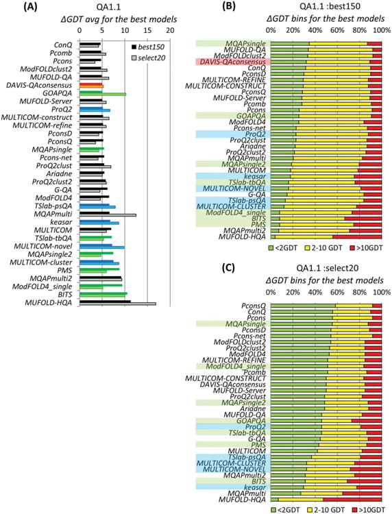
Ability of the QA predictors to identify the best models in the decoy sets. The analysis was carried out on the 74 /75 targets, for which at least one structural model had a GDT_TS score over 40 in the S20 /B150 datasets, respectively. Coloring of the methods is the same as in Figure 1. (A) Average difference in quality between the models predicted to be the best and the actual best models. For each group, ΔGDT_TS scores are calculated for every target, and averaged over all predicted targets in every dataset. The lower the score, the better the group's performance. (B, C) Stacked bars showing the percentage of predictions where the model estimated to be the best in B150 (B) and S20 (C) datasets, is 0–2, 2–10 and >10 GDT_TS units away from the actual best model. Groups are sorted according to the results in the 0–2 bin (green bars).

Average ΔGDT_TS scores for groups submitting quality estimates on at least ¾ of the targets for which the B150 /S20 datasets contained at least one good structural model (GDT_TS>40) are presented in Figure 2(A). The best selectors could identify the best models with an average error of 4.6 GDT_TS units on the B150 datasets and 3.4 GDT_TS units on the S20 sets. Average ΔGDT_TS scores for the majority of groups appeared to be similar on both types of datasets, except for three groups that showed substantially poorer results on the S20 set. It is encouraging to see a single-model method (ProQ2) among the “best selectors” and scoring just slightly worse than the reference Davis-QAconsensus approach. Also, it is interesting to note that the ConQ method does relatively well in this aspect of assessment, while it shows a rather average performance in the correlation-based evaluation. It should be mentioned though, that the results of all top performing methods are indistinguishable from each other and from the reference clustering method according to the statistical significance tests (see Table S3 in Supporting Information).

Panels B and C in Figure 2 show the percentage of targets, for which the models identified as best in the B150 and S20 datasets, respectively, were within 2, 10, and more than 10 GDT_TS units away from the best available models. It can be seen that the best predictors can identify the best model within 2 GDT_TS units for only approximately one in three targets on the B150 sets and for slightly more than every other target on the S20 sets. It should be mentioned, though, that the selectors' job on the B150 datasets was more challenging as the spread in model quality was smaller and thus it was harder to pick the best model; for the same reason, the predictors were less likely to miss the best model by much on these datasets. In general, the average scores for the best 12 predictors in “green” and “red” bins are larger for the S20 datasets (54 and 12%, correspondingly) than for the B150 sets (30 and 10%, respectively).

Ability to distinguish between good and bad models

The ability of predictors to discriminate between good and bad models was assessed using a Receiver Operating Characteristic (ROC) analysis and by calculating the Matthews Correlation Coefficients (MCC) (Fig. 3). Group rankings from the two approaches appeared to be very similar and therefore we only show in this section the results from the ROC analysis. The MCC-based results are discussed below in the context of the comparison of the CASP10 assessment data with those from the previous CASP.

Figure 3.

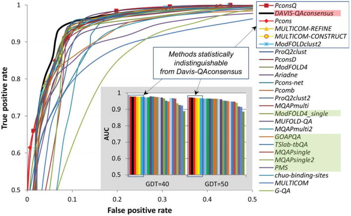
ROC curves for the binary classifications of models into two classes: good (GDT_TS ≥ 50) and bad (otherwise). Group names are provided as a top-to-bottom list ordered according to decreasing AUC scores. Group name's background differentiates different types of methods according to the coloring scheme in Figure 1 (clustering methods have transparent background). Statistically indistinguishable groups are boxed in the legend and provided with data markers. The data for the reference consensus method are plotted as a thicker black line. The data are shown for the best 25 groups only. For clarity, only the left upper quarter of a typical ROC curve plot is shown (FPR ≤ 0.5, TPR ≥ 0.5). The inset shows the AUC scores for all groups, and for two different definitions of model correctness: GDT_TS ≥ 40 and GDT_TS ≥ 50.

Figure 3 shows the ROC curves for the participating groups on the B150 datasets assuming a threshold of GDT_TS=50 for the separation between good and bad models. The ROC curves for the top performing groups are very similar to each other, suggesting that the corresponding methods have similar discriminatory power. Comparing the AUC scores for the GDT_TS=40 and GDT_TS=50 thresholds (see the two panels in the inset of Fig. 3) one can see that the results are rather insensitive to the selected cutoff. According to the results of nonparametric DeLong tests (see Table S2, panel B in Supporting Information) the reference Davis-QAconsensus method is statistically indistinguishable from the top 5 groups (all clustering approaches) and better than all other groups.

Ability to assign proper error estimates to the modeled residues

For the nineteen groups that submitted model confidence estimates at the level of individual residues (QA2), we measured the correlation between predicted and observed distance errors, setting all values exceeding 5Å to 5Å.¹⁰

Panels A and B in Figure 4 show the mean z-scores and PMCC weighted means for the participating QA2 groups on the B150 and S20 model sets, respectively. Two methods - Pcons and Pcomb - achieve the highest scores on both datasets. These groups are statistically indistinguishable from each other and from two other groups – PconsQ and ModFOLDclust2 (see Supporting Information Table S4), and differ from the remaining QA2 groups. Comparing scores for the same groups on the two datasets, we notice that they are very similar indicating that the performance of the local quality assessment methods is largely insensitive to the input datasets in CASP.

Figure 4.

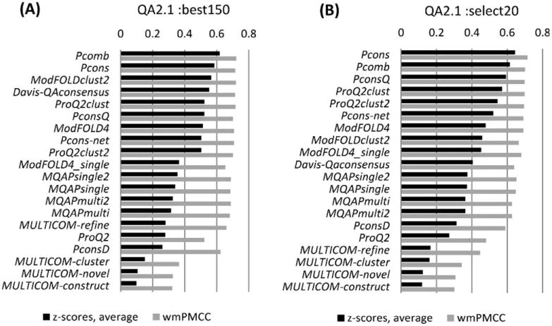
Correlation analysis for 19 individual groups and the Davis-QAconsensus reference method for the per-residue quality prediction category. Correlation analysis results are calculated on a per-model basis and subsequently averaged over all models and all targets in the B150 (A) and S20 (B) datasets.

Ability to discriminate between good and bad regions in the model

To evaluate the accuracy with which the correctly predicted regions are identified, we pooled the submitted estimates for all residues from all models and all targets (over 3,300,000 residues from over 14,000 of models per QA predictor in B150 datasets and ∼500,000 residues from 1,900 models in S20 sets) (Fig. 5). For these residues we calculated the Matthews correlation coefficient and carried out the ROC analysis (see Materials in this and CASP9 papers for details of the procedures). Similarly to global classifiers (i.e., good/bad model), the ranking of local classifiers (reliable/unreliable residues) appears to be very similar according to the two aforementioned approaches, and we describe here the ROC analysis - the MCC data will be shown in the comparison with results from previous CASP.

Figure 5.

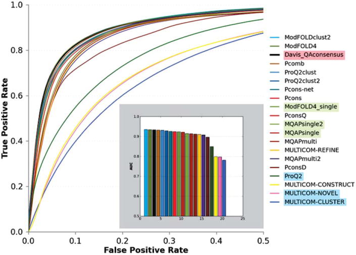
Accuracy of the binary classifications of residues (reliable/unreliable) based on the results of the ROC analysis. A residue in a model is defined to be correct when its Cα is within 3.8Å from the corresponding residue in the model. Group names are provided as a top-to-bottom list ordered according to decreasing AUC scores. Group name's background differentiates different types of methods according to the coloring scheme in Figure 1 (clustering methods have transparent background). The data for the reference consensus method are plotted as a thicker black line. For clarity, only the left half of a typical ROC curve plot is shown (FPR ≤ 0.5). The inset shows the AUC scores for all groups.

Figure 5 demonstrates that two groups, ModFOLDclust2 and ModFOLD4, are on top of the list of the local classifiers. These two groups show statistically similar results to those of the reference Davis_QAconsensus method and to the two next groups in the ranking – Pcomb and ProQ2clust (see Table S5 in the Supporting Information). In general, the difference between predictors in terms of the AUC is very small. One can notice that all top performing methods are developed in three research groups led by L.McGuffin (University of Reading, UK), B.Wallner (Linkoping University, Sweden) and A.Elofsson (Stockholm University, Sweden), and that all the top-performing groups use clustering approaches, while the best single-model method performs significantly worse.

Ability to self-assess the reliability of model coordinates in TS modeling

To evaluate the ability of TS predictors to assign realistic error estimates to the coordinates of their own models, we computed the log-linear Pearson correlation between the observed and predicted residue errors, and performed a ROC analysis. The assessment was performed separately for all participating groups on a subset of “all-group” targets (Fig. 6), and for server predictors – on all targets (Figs. S1 and S2 in Supporting Information).

In CASP10, out of 150 participating TS methods only 67 provided per-residue confidence estimates and only six methods (developed by only two different research groups) were able to provide reasonable estimates. These methods attained correlation coefficients above 0.58 and AUC values above 0.8, outperforming other predictors to a significant extent (see Panels A and B in Fig. 6). Panels C and D visualize the striking difference between one of the leading groups, TS273, and group TS388 that ranks immediately after the best six. One can easily notice a quite good correlation between the observed and predicted values in Panel A, and essentially no correlation in the data shown in panel B. The best server method, IntFOLD2, reaches the highest correlation coefficients of 0.70 [0.78] on all-group [all-group + server-only] targets, and outperforms all other methods in all evaluation modes in a statistically significant manner (see Table S6 in Supporting Information). The only exception is another server method developed by the same research group (IntFOLD) that performs equally well in the ROC analysis on the “all-group” targets. The two aforementioned servers are by far better than all other server QA3 estimators also according to the results of the DeLong tests and Z-tests (notice the large absolute values of Z-statistics in Supporting Information Table S6).

In order to provide a baseline estimate of the accuracy of the QA3 predictions, we compared them with the perresidue quality estimates provided by the two best performing CASP9¹⁰ single-model MQA methods: ProQ2 ¹⁷ and QMEAN¹⁸. Figure 6(B) demonstrates that these baseline methods are better than all but six methods (all using clustering QA techniques) on the human/server targets, while Figure S2 in Supporting Information shows them losing to only the two QA3 server methods mentioned in the previous paragraph on all targets.

As the QA2 and QA3 categories are conceptually similar, it is not surprising to notice that the best-performing predictors in the QA3 category were developed at the same centers as mentioned in the previous section. Strikingly, most of the top-ranking groups in the assessment of tertiary structure prediction [Refs: TBM paper - this issue, FM paper - this issue] are not providing realistic error estimates for their predictions, which seriously limits the usefulness of these methods, and their appropriateness for real-life applications.

Comparison with the previous CASP

Figure 7 provides at a glance comparison of various aspects of CASP10 and CASP9 assessments. It should be noted, though, that the results of the direct comparison should be interpreted with caution, as the three test sets analyzed here were conceptually different—the CASP9 dataset contained all server models and therefore was larger and more diverse in terms of quality of models than the two CASP10 datasets (see Materials).

Figure 7.

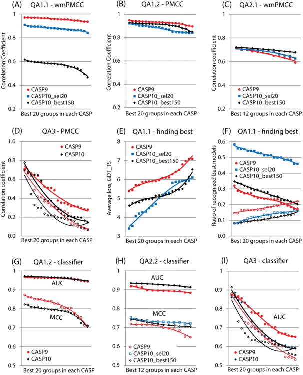
Comparison of the results of the best 20 groups (QA1) and the best 12 groups (QA2, QA3) in the last two CASPs according to various evaluation metrics. Groups are sorted from best to worst in each CASP. (A-D) Correlation coefficients in (A) QA1.1, (B) QA1.2, (C) QA2.1 and (D) QA3 evaluation modes. Filled data markers and bolder trendlines in the QA3 analysis (panels D and I) correspond to the assessment of all methods, while hollow markers and thinner trendlines to server only methods. (E-F) Ability of predictors to identify the best model: (E) average loss in quality due to nonoptimal selection, (F) ratios of recognized and missed best models (filled data markers and bolder trendlines: percentage of models recognized within 2 GDT_TS units; hollow markers and thinner trendlines: models missed by more than 10 GDT_TS units). (G-I) Success of predictors in distinguishing between (G) good and bad models, and (H, I) correctly and incorrectly modeled regions in the QA2.2 (H) and QA3 (I) evaluation modes. The thresholds for defining a “correct” model/residue for the MCC and AUC calculations were set to 50 GDT_TS for the global classifier assessment (panel G) and to 3.8 Å for the local classifier assessment (panels H and I).

Panels A through D show the correlation between the observed and predicted scores for the best groups participating in the last two CASPs. It can be seen that the correlation coefficients from the global per-target assessment (Panel A) are lower for CASP10 than for CASP9. This is especially true for the CASP10 B150 datasets, which have the narrowest spread of model quality and appear to be the most challenging. At the same time, the CCs in the “ all models pooled together ” assessment (Panel B) and in the per-residue error estimate assessment (Panel C) are very similar on both sets of CASP10 and on the CASP9 dataset. In the self-assessment (Panel D), results in both CASPs are in general very poor with median PMCC around 0.1. Correlation scores for all groups other than the best six and for server groups other than the best two are noticeably worse in CASP10, dropping below the 0.5 level. The top six methods in two recent CASPs originate from the same two research centers and show approximately the same correlation ranging from 0.57 to 0.71. The best server group - IntFOLD2 showed a significantly improved correlation on all targets (0.78 in CASP10 vs. 0.69 in CASP9), which is an important step towards more reliable model error estimates.

Panels E and F summarize the progress in identifying the best models. The CASP10 curves in panel E are lower than those of CASP9, indicating a better accuracy in recognizing the best models in the present experiment. The data in panel F confirm this result showing that the best CASP10 predictors were more often able to identify the best model correctly (higher bolder lines) and less often missed the best model by much (lower thinner lines). Unfortunately, this result cannot be directly attributed to the improved performance as the CASP10 datasets had a smaller spread of model quality and therefore methods participating in CASP10 had a smaller chance of selecting a wrong model.

Panels G through I compare the ability to distinguish between the well and not so well modeled structures and their regions. From the graphs in panels G and H, it is difficult to detect any improvement in the two-class classifier performance of prediction methods either by the MCC or AUC measures. Similarly to what we have observed for the other measures, the results of the best groups did not improve. This comparison can be taken with higher confidence since all CASP9 and CASP10 “all models pooled together” datasets contained enough data points (either models or residues) and represented the full spectrum of quality. Similarly to the correlation analysis, the quality of the two-class classifiers in the QA3 mode (Panel I) is approximately the same for the six best methods in both CASPs and deteriorates fast for the methods outside this set of groups, with the CASP10 scores falling off faster than their counterparts in CASP9.

Conclusions

State-of-the-art in protein model quality assessment was tested in CASP10 with a new two-stage procedure. Methods were probed for their ability to assign quality annotations to models from small but quite diverse datasets as well as from a large but more uniform dataset. With the new assessment protocol in place, the correlation achieved by the best groups dropped from 0.97 in CASP9 to 0.6 in CASP10 (on the best 150 models datasets). On the contrary, local quality assessment methods appeared to be practically insensitive to the input data – their performance is stable across different datasets and CASP experiments. Single- and quasi-single-model methods appeared to be more competitive with pure clustering techniques, which nevertheless, were shown to hold ground even in the cases where only a few diverse models were made available. This is quite an important result as many specialists in the area, including the assessors and method developers, tended to believe that twenty models were too few for clustering methods to operate effectively, and therefore considered clustering techniques of limited practical use. It still may be the case that the twenty CASP models represent a lesser challenge than a real-life 20 model set, as the latter most likely will have a narrower quality spread. To further explore the impact of the dataset size on clustering methods, we are planning to reduce the number of models in the CASP11 stage_1 dataset even further (to ten), and to introduce an additional dataset with fewer than 150 similar models. On the basis of the community reaction to the suggested changes and the results presented here we will decide which datasets to use for the CASP11 testing.

In the majority of the CASP10 analyses, the evaluation scores for the top twelve MQA methods appeared to be statistically indistinguishable from one another indicating approximately similar performance of the best groups. These scores are also similar to those of the reference clustering method, as no QA method could outperform the reference method in a statistically significant way.

Despite the fact that the best methods can attain high correlation coefficients for some targets, none of them can consistently select the best models. At the same time, some of the methods that on the average are quite poor in ranking models appeared to be among the best in picking the best models from the decoy sets. Also, for the second CASP in a row, a single-model method performed among the best in this category.

Single-model methods in general are a rarity in CASP. Only five methods of this kind participated in CASP10 and we would very much like to see this number increased in the future round of CASP. Similarly, we encourage the community to pay more attention to per-residue quality assessment methods, as currently such methods are developed in only four scientific centers.

As in previous CASPs, the evaluation of tertiary structure error estimates (self-assessment) in CASP10 exposed a regrettable state of the affairs in this category, as only a small fraction of all predictor groups provide error estimates for their predictions, and only two research groups seem to be actively addressing this issue. Given the usefulness of model quality estimates in judging the suitability of a model in practical applications, this is likely to lessen the impact of structure prediction in the life sciences. During the CASP10 predictors meeting, several participants suggested including model confidence values as a prerequisite for participation in the future CASP experiments in order to encourage more development in this area.

Abbreviations

CC

Correlation Coefficient

B150

“Best 150” – a dataset comprised of the best 150 models submitted on a target according to the benchmark consensus method

GDT_TS

Global Distant Test – Total Score

MCC

Matthews' Correlation Coefficient

wmPMCC

weighted mean of PMCC

MQA

Model Quality Assessment

PMCC

Pearson's product-Moment Correlation Coefficient

QA1.1

per-target global quality assessment

QA1.2

all models pooled together global quality assessment

QA2.1

per-target local quality assessment

QA2.2

all models pooled together local quality assessment

QA3

self-assessment of residue error estimates

ROC

Receiver Operating Characteristic

S20

“Selected 20” – a dataset comprised of 20 models spanning the whole range of server model difficulty on each target

TS

Tertiary Structure

References

- 1.Schwede T, Sali A, Honig B, Levitt M, Berman HM, Jones D, Brenner SE, Burley SK, Das R, Dokholyan NV, Dunbrack RL, Jr, Fidelis K, Fiser A, Godzik A, Huang YJ, Humblet C, Jacobson MP, Joachimiak A, Krystek SR, Jr, Kortemme T, Kryshtafovych A, Montelione GT, Moult J, Murray D, Sanchez R, Sosnick TR, Standley DM, Stouch T, Vajda S, Vasquez M, Westbrook JD, Wilson IA. Outcome of a workshop on applications of protein models in biomedical research. Structure. 2009;17:151–159. doi: 10.1016/j.str.2008.12.014. [DOI] [PMC free article] [PubMed] [Google Scholar]
- 2.Moult J. Comparative modeling in structural genomics. Structure. 2008;16:14–16. doi: 10.1016/j.str.2007.12.001. [DOI] [PubMed] [Google Scholar]
- 3.Tramontano A. The role of molecular modelling in biomedical research. FEBS Lett. 2006;580:2928–2934. doi: 10.1016/j.febslet.2006.04.011. [DOI] [PubMed] [Google Scholar]
- 4.Moult J, Fidelis K, Kryshtafovych A, Tramontano A. Critical assessment of methods of protein structure prediction (CASP)-round IX. Proteins. 2011;79(Suppl 10):1–5. doi: 10.1002/prot.23200. [DOI] [PMC free article] [PubMed] [Google Scholar]
- 5.Kryshtafovych A, Fidelis K, Moult J. CASP9 results compared to those of previous casp experiments. Proteins. 2011;79(Suppl 10):196–207. doi: 10.1002/prot.23182. [DOI] [PMC free article] [PubMed] [Google Scholar]
- 6.Pieper U, Webb BM, Barkan DT, Schneidman-Duhovny D, Schlessinger A, Braberg H, Yang Z, Meng EC, Pettersen EF, Huang CC, Datta RS, Sampathkumar P, Madhusudhan MS, Sjolander K, Ferrin TE, Burley SK, Sali A. ModBase, a database of annotated comparative protein structure models, and associated resources. Nucleic Acids Res. 2011;39(Database issue):D465–D474. doi: 10.1093/nar/gkq1091. [DOI] [PMC free article] [PubMed] [Google Scholar]
- 7.Arnold K, Kiefer F, Kopp J, Battey JN, Podvinec M, Westbrook JD, Berman HM, Bordoli L, Schwede T. The Protein Model Portal. J Struct Funct Genomics. 2009;10:1–8. doi: 10.1007/s10969-008-9048-5. [DOI] [PMC free article] [PubMed] [Google Scholar]
- 8.Kiefer F, Arnold K, Kunzli M, Bordoli L, Schwede T. The SWISS-MODEL Repository and associated resources. Nucleic Acids Res. 2009;37(Database issue):D387–D392. doi: 10.1093/nar/gkn750. [DOI] [PMC free article] [PubMed] [Google Scholar]
- 9.Kryshtafovych A, Fidelis K. Protein structure prediction and model quality assessment. Drug Discov Today. 2009;14(7/8):386–393. doi: 10.1016/j.drudis.2008.11.010. [DOI] [PMC free article] [PubMed] [Google Scholar]
- 10.Kryshtafovych A, Fidelis K, Tramontano A. Evaluation of model quality predictions in CASP9. Proteins. 2011;79(Suppl 10):91–106. doi: 10.1002/prot.23180. [DOI] [PMC free article] [PubMed] [Google Scholar]
- 11.Cozzetto D, Kryshtafovych A, Tramontano A. Evaluation of CASP8 model quality predictions. Proteins. 2009;77(Suppl 9):157–166. doi: 10.1002/prot.22534. [DOI] [PubMed] [Google Scholar]
- 12.Cozzetto D, Kryshtafovych A, Ceriani M, Tramontano A. Assessment of predictions in the model quality assessment category. Proteins. 2007;69(Suppl 8):175–183. doi: 10.1002/prot.21669. [DOI] [PubMed] [Google Scholar]
- 13.Chen VB, Arendall WB, 3rd, Headd JJ, Keedy DA, Immormino RM, Kapral GJ, Murray LW, Richardson JS, Richardson DC. MolProbity: all-atom structure validation for macromolecular crystallography. Acta Crystallogr D Biol Crystallogr. 2010;66(Part 1):12–21. doi: 10.1107/S0907444909042073. [DOI] [PMC free article] [PubMed] [Google Scholar]
- 14.Wiederstein M, Sippl MJ. ProSA-web: interactive web service for the recognition of errors in three-dimensional structures of proteins. Nucleic Acids Res. 2007;35(Web Server issue):W407–W410. doi: 10.1093/nar/gkm290. [DOI] [PMC free article] [PubMed] [Google Scholar]
- 15.Zemla A. LGA: a method for finding 3D similarities in protein structures. Nucleic Acids Res. 2003;31:3370–3374. doi: 10.1093/nar/gkg571. [DOI] [PMC free article] [PubMed] [Google Scholar]
- 16.Tai E, Taylor T, Bai H, Montelione G, Lee B, et al. Target definition and classification in CASP10. Proteins. 2013 doi: 10.1002/prot.24434. THIS ISSUE. [DOI] [PMC free article] [PubMed] [Google Scholar]
- 17.Ray A, Lindahl E, Wallner B. Improved model quality assessment using ProQ2. BMC Bioinformatics. 2012;13:1. doi: 10.1186/1471-2105-13-224. [DOI] [PMC free article] [PubMed] [Google Scholar]
- 18.Benkert P, Biasini M, Schwede T. Toward the estimation of the absolute quality of individual protein structure models. Bioinformatics. 2011;27:343–350. doi: 10.1093/bioinformatics/btq662. [DOI] [PMC free article] [PubMed] [Google Scholar]
- 19.Mariani V, Kiefer F, Schmidt T, Haas J, Schwede T. Assessment of template based protein structure predictions in CASP9. Proteins. 2011;79(Suppl 10):37–58. doi: 10.1002/prot.23177. [DOI] [PubMed] [Google Scholar]
- 20.Levitt M, Gerstein M. A unified statistical framework for sequence comparison and structure comparison. Proc Natl Acad Sci USA. 1998;95:5913–5920. doi: 10.1073/pnas.95.11.5913. [DOI] [PMC free article] [PubMed] [Google Scholar]
- 21.Wallner B, Elofsson A. Prediction of global and local model quality in CASP7 using Pcons and ProQ. Proteins. 2007;69(Suppl 8):184–193. doi: 10.1002/prot.21774. [DOI] [PubMed] [Google Scholar]
- 22.McGuffin LJ. Prediction of global and local model quality in CASP8 using the ModFOLD server. Proteins. 2009;77(Suppl 9):185–190. doi: 10.1002/prot.22491. [DOI] [PubMed] [Google Scholar]
- 23.Zhou H, Skolnick J. GOAP: a generalized orientation-dependent, all-atom statistical potential for protein structure prediction. Biophys J. 2011;101:2043–2052. doi: 10.1016/j.bpj.2011.09.012. [DOI] [PMC free article] [PubMed] [Google Scholar]
- 24.McGuffin LJ. The ModFOLD server for the quality assessment of protein structural models. Bioinformatics. 2008;24:586–587. doi: 10.1093/bioinformatics/btn014. [DOI] [PubMed] [Google Scholar]
- 25.Roche DB, Buenavista MT, Tetchner SJ, McGuffin LJ. The IntFOLD server: an integrated web resource for protein fold recognition, 3D model quality assessment, intrinsic disorder prediction, domain prediction and ligand binding site prediction. Nucleic Acids Res. 2011;39:W171–176. doi: 10.1093/nar/gkr184. [DOI] [PMC free article] [PubMed] [Google Scholar]
- 26.McGuffin LJ, Roche DB. Rapid model quality assessment for protein structure predictions using the comparison of multiple models without structural alignments. Bioinformatics. 2010;26:182–188. doi: 10.1093/bioinformatics/btp629. [DOI] [PubMed] [Google Scholar]
- 27.Wang Q, Vantasin K, Xu D, Shang Y. MUFOLD-WQA: a new selective consensus method for quality assessment in protein structure prediction. Proteins. 2011;79(Suppl 10):185–195. doi: 10.1002/prot.23185. [DOI] [PMC free article] [PubMed] [Google Scholar]
- 28.Wang Z, Tegge AN, Cheng J. Evaluating the absolute quality of a single protein model using structural features and support vector machines. Proteins. 2009;75:638–647. doi: 10.1002/prot.22275. [DOI] [PubMed] [Google Scholar]
- 29.Larsson P, Skwark MJ, Wallner B, Elofsson A. Assessment of global and local model quality in CASP8 using Pcons and ProQ. Proteins. 2009 doi: 10.1002/prot.22476. [DOI] [PubMed] [Google Scholar]
- 30.Wallner B, Larsson P, Elofsson A. Pcons.net: protein structure prediction meta server. Nucleic Acids Res. 2007;35(Web Server issue):W369–W374. doi: 10.1093/nar/gkm319. [DOI] [PMC free article] [PubMed] [Google Scholar]
- 31.Ray A, Lindahl E, Wallner B. Improved model quality assessment using ProQ2. BMC Bioinformatics. 2012;13:224. doi: 10.1186/1471-2105-13-224. [DOI] [PMC free article] [PubMed] [Google Scholar]
Associated Data
This section collects any data citations, data availability statements, or supplementary materials included in this article.