Autonomous Unobtrusive Detection of Mild Cognitive Impairment in Older Adults

Abstract

The current diagnosis process of dementia is resulting in a high-percentage of cases with delayed detection. To address this problem, in this paper we explore the feasibility of autonomously detecting mild cognitive impairment (MCI) in the older adult population. We implement a signal processing approach equipped with a machine learning paradigm to process and analyze real world data acquired using home-based unobtrusive sensing technologies. Using the sensor and clinical data pertaining to 97 subjects, acquired over an average period of 3 years, a number of measures associated with the subjects' walking speeds and general activity in the home were calculated. Different time spans of these measures were used to generate feature vectors to train and test two machine learning algorithms namely support vector machines and random forests. We were able to autonomously detect MCI in older adults with an area under the ROC curve of 0.97 and an area under the precision-recall curve of 0.93 using a time window of 24 weeks. This work is of great significance since it can potentially assist in the early detection of cognitive impairment in older adults.

I. Introduction

PEOPLE aged 65 and older constitute the fastest growing population segment in North America, Europe, and Asia. According to the US Census Bureau, the global number of adults over the age of 60 is expected to reach 1.2 billion by the year 2025 [1]. In Canada, the proportion of Canadians aged 65 and over is expected to represent 26.4% of the total population by the year 2031 [2]. This statistic poses a serious problem to the health care system since older adults possess a higher propensity to suffer from chronic illnesses or dementia. Statistics show that 1 in 11 Canadians over the age of 65 has Alzheimer's disease, and given that the Canadian population is aging, in just 5 years, as many as 50% more Canadian families could be facing Alzheimer's disease or another dementia [3].

Although clinical tests and procedures for diagnosing dementia have been very accurate in identifying dementia, studies have shown that there is a high degree of underrecognition of dementia [4]. Those studies have shown that in more than 50% of the cases, it is the family members who serve as the source of primary recognition and not the general practice physicians. This delay in detecting dementia can have detrimental effects especially to subjects with reversible forms of dementia, who form up to 11% of the cognitively impaired population, since failing to recognize some of these causes early might lead to irreversible damage [5]. Therefore, early detection of dementia is of great significance because it increases the chances of successfully reversing the cause of dementia. In addition, for subjects with irreversible dementia, although no treatment exists, early detection of dementia still provides them and their families with an opportunity to proactively plan for their future. They can seek the appropriate interventions that enhance daily functioning and safety of the impaired member and that reduce any emotional stress and individual fear [6]. However, early detection of dementia can be very challenging with the contemporary detection process.

Current detection process starts by general practice physicians referring patients to memory clinics for cognitive assessments after repeated reports of memory problems by the patients themselves, family members, or caregivers. In memory clinics, cognition of patients is assessed using questionnaires, screening tools, and episodic examinations of cognitive capacity such as the Montreal Cognitive Assessment (MoCA) [7], the Mini-Mental State Examination (MMSE) [8], and the Clinical Dementia Rating (CDR) [9]. However, the detection process suffers from inherent shortcomings. First, some studies have found that older adults or families reported memory problems in only a small percentage of cases in which the older adult had been clinically labeled as cognitively impaired [10]. This could be because older adults might be unaware of their impairment, or if noted, might be uncomfortable discussing their concerns. Also, people cannot recall with high fidelity meaningful changes that are infrequent and brief in duration or subtle and evolving slowly over time. Accordingly, older adults may fail to sufficiently identify key transient events which because of their infrequent occurrence may be easily forgotten [11]. As for questionnaires and episodic in-person examinations, they depend on a snapshot observation of function and assume that observations recorded during the examination represent the person's typical state of function and cognition for relatively long periods of time prior to the assessment [12]. Consequently, an alternative approach is to bring assessment into the daily activity of a person in their home environment preferably via unobtrusive sensors and smart systems.

The rest of the paper is organized as follows: Section II summarizes related work, lists research questions, and presents contributions. Section III sets up the problem and introduces a general overview of the proposed cognitive status recognition methodology. Section IV describes the data and how they were acquired, and the measures and the features that were computed and experimented with. Section V presents and discusses the results obtained. Section VI addresses the limitations of the current work and discusses potential future work. Finally, Section VII concludes the paper.

II. Related Work

The use of technology in developing systems that promote older adults' independence and aging-in-place has been well-received by many caregivers, clinicians, older adults, and family members [13] [14]. This along with recent advances in technology has lead to the proliferation of smart homes. Literature contains a plethora of published studies on smart homes such as the Microsoft's EasyLiving project [15], the GATOR Tech Smart House [16], the AWARE home at Georgia Tech [17], the MavHome Project at the University of Texas at Arlington [18], and the GE QuietCare System [19], and other works that have attempted to detect early changes in health using unobtrusive sensors such as [20]. All these published studies endeavor to promote older adults' independence by automating repetitive tasks carried out by the inhabitants of these homes. Some studies were also able to detect general changes in daily activities which could indicate a potential change in health. All respective results reported in the literature were based on data acquired in a laboratory environment and not in a real world setting.

The most recent smart home that addressed discriminating older adults with cognitive impairment is the CASAS project at the Washington State University. In their latest study, the CASAS group used a machine learning approach to detect cognitive impairment in about 179 older adults based on their ability to complete ‘Day Out Task’, that consisted of carrying out eight Instrumental Activities of Daily Living (IADL) that might be interwoven [21] [22]. Data acquisition was conducted in the CASAS testbed. Machine Learning algorithms were employed to discriminate older adults with cognitive impairment from cognitively intact older adults based on several features that were computed from the sensor data. The results reported were based on subjects carrying out the task in a laboratory environment and not a real world setting. However, an approach that would be more reflective of the subjects' actual performance would be continuous monitoring of the subjects' ability to complete the task over several trials, perhaps in their home since this would capture their true performance.

The ORegon Centre for Aging and TECHnology (ORCAT-ECH) at the Oregon Health and Science University (OHSU) developed and pilot tested the first community-wide, scalable home-based assessment platform and protocol. They employed unobtrusive sensing technologies in the homes of at least 300 cognitively healthy older adults for an average period of 3 years, resulting in a large database of sensor data and clinical data. In their latest work [23], Dodge et al. presented for the first time trajectories of home-based daily walking speeds and their variability, associated with the recruited subjects over 3 years. According to Dodge et al., participating older adults with non-amnestic mild cognitive impairment (naMCI) were characterized by a slowing of walking speed. Furthermore, older adults with naMCI exhibited the highest and lowest variability in their walking speeds in comparison with the participating cognitively intact older adults.

Walking speed and variability of walking speed have been found, in different works [24] [25] [26], to be good measures in differentiating older adults with MCI and cognitive decline syndromes. Accordingly, our work explores the following research questions:

1. Can we use signal processing along with machine learning techniques to autonomously detect older adults with mild cognitive impairment (MCI) using predefined measures calculated from unobtrusive sensing technologies?

2. What time span of predefined measures results in the highest areas under the ROC curve and the precision-recall curve?

3. How do features extracted from these predefined measures rank in terms of their importance for detection of mild cognitive impairment?

To answer these questions, by collaborating with OR-CATECH, we were able to access sensor and clinical data corresponding to 97 homes with singe occupants collected over an average period of 3 years in the subjects' homes. Several predefined measures associated with the subjects' weekly walking speeds and general activity in the home were used to train and test two machine learning algorithms namely support vector machines (SVM) and random forests (RF). This paper makes the following contributions:

1. We demonstrate how a signal processing approach equipped with a machine learning paradigm can be used to discriminate older adults with MCI from their cognitively healthy counterparts using several predefined measures associated with the subjects' walking speeds and general activity in the home.

2. We demonstrate that by analyzing a time window of only 24 weeks we can detect older adults with MCI with areas under the ROC curve and the precision-recall curve of 0.97 and 0.93, respectively.

3. We further analyze the measures and their respective features and rank them in a descending order based on their importance for detection of cognitive impairment.

4. Finally, we take the lead in reporting these promising results using real-world data suffering from too much noise and missing many datapoints. Almost all of the other related work in the literature, by contrast, have reported results obtained by carrying out activities and analyzing data acquired in a laboratory setting which might not have necessarily reflected the real performance of the subjects.

III. Problem Setup

Suppose that a database consists of N subjects being continuously monitored in their homes using unobtrusive sensing technologies, and for each subject, p weekly measure vectors exist. A weekly measure vector v is basically a vector of values, such as median walking speed and coefficient of variation of walking speed, calculated over a period of one week from the sensing technologies. Given this database of measure vectors, we are interested in autonomously labeling these vectors as belonging to subjects who are cognitively intact or to subjects suffering from MCI. We are formulating the problem as a classification problem with two classes: cognitive intactness and MCI. In this work, we refer to the MCI class as ‘positive’ class and the cognitive intactness class as ‘negative’ class, and will be using them interchangeably depending on the context. Also, we represent vectors by bold lower case letters, e.g. v, matrices by bold upper case letters, e.g. V, and sets by calligraphic uppercase letters, V. Mathematically, the cognitive status recognition problem can be formulated as follows: The database consists of N subjects, each having p measure vectors, tabulated as the following sets,

$$\begin{array}{c}{\mathcal{M}}_1=\{{\mathbf{v}}_{1,1},{\mathbf{v}}_{1,2},\dots ,{\mathbf{v}}_{1,p1}\},\\ {\mathcal{M}}_2=\{{\mathbf{v}}_{2,1},{\mathbf{v}}_{2,2},\dots ,{\mathbf{v}}_{2,p2}\},\\ ⋮\\ {\mathcal{M}}_N=\{{\mathbf{v}}_{N,1},{\mathbf{v}}_{N,2},\dots ,{\mathbf{v}}_{N,pN}\}.\end{array}$$ (1)

Each v_i,j is an R-dimensional vector where R is the number of measures calculated from the sensor data as shown in Fig. 1. Note that R is the same for all vectors among all subjects but the number of weekly measure vectors p can be different among subjects since subjects can be monitored for different periods. Hence, the subscript i in p_i indicates the subject number.

Fig. 1.

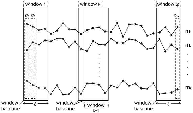
Trajectories of weekly measures pertaining to subject i in the database. Each asterisk represents a weekly measure. Features are extracted using a window of size ℓ, that slides one week at a time.

Fig. 2 depicts the general overview of the proposed approach in recognizing the subjects' cognitive status. Using a sliding window of size ℓ (in weeks), the measure vectors are transformed into feature vectors. The resulting feature space can be tabulated as the following sets,

Fig. 2.

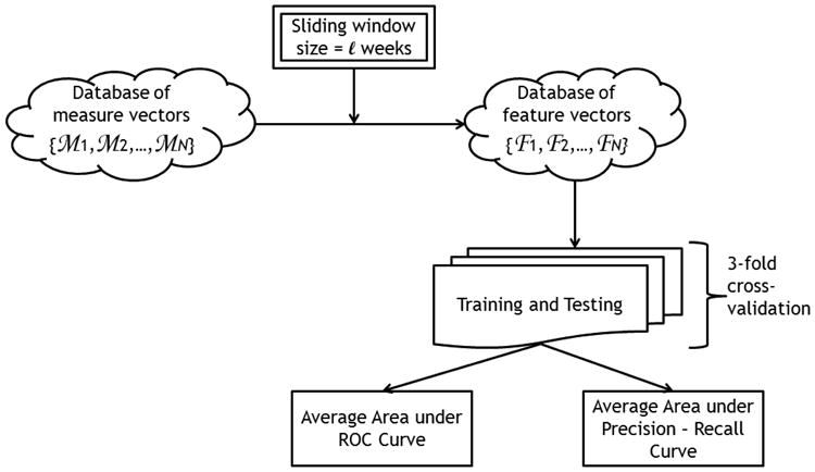
General overview of the cognitive status recognition process.

$$\begin{array}{c}{\mathcal{F}}_1=\{{\mathbf{w}}_{1,1},{\mathbf{w}}_{1,2},\dots ,{\mathbf{w}}_{1,q1}\},\\ {\mathcal{F}}_2=\{{\mathbf{w}}_{2,1},{\mathbf{w}}_{2,2},\dots ,{\mathbf{w}}_{2,q2}\},\\ ⋮\\ {\mathcal{F}}_N=\{{\mathbf{w}}_{N,1},{\mathbf{w}}_{N,2},\dots ,{\mathbf{w}}_{N,qN}\}.\end{array}$$ (2)

Note that for ℓ ≥ 1 week, the resulting number of feature vectors for subject i, q_i, will be less than the corresponding number of measure vectors, p_i. In this work, each feature vector represents a datapoint. Note that the number of feature vectors, or datapoints, for each subject is different for each ℓ. Also, note that each w_i,j can have different dimensions depending on the feature type. For example, if the feature type selected is the average of the individual measures in a window, then each w_i,j would be an R-dimensional vector. On the other hand, if the feature type selected is a concatenation of the trajectories of the individual measures in a window for example, then w_i,j would be an (R × ℓ)-dimensional vector.

For each window size ℓ, the generated feature vectors are then used to train and test a machine learning algorithm using the following procedure. The database of feature vectors is first divided into three groups of subjects, each group containing approximately the same number of feature vectors pertaining to each class: positive class and negative class. Since subjects can be monitored for different periods, which in turn results in subjects having different numbers of datapoints, then each group does not necessarily contain the same number of subjects. However, all three groups are created such that each group has approximately the same number of datapoints pertaining to each class. Then the performance of the machine learning algorithm is evaluated through a 3-fold cross-validation process, that consists of three runs. In each run, two groups are used to train the algorithm and the third group is used to test it. Accordingly, in each run, the algorithm is tested on datapoints it has not seen in the training phase. Using this methodology, the algorithm eventually yields a prediction for each datapoint. As depicted in Fig. 2, performance is quantified by generating the ROC curve and the precision-recall curve and calculating the areas under them, AUC_SS and AUC_PR respectively, where,

$$\text{sensitivity}=\frac{\text{TP}}{\text{TP}+\text{FN}},$$ (3)

$$\text{specificity}=\text{recall}=\frac{\text{TN}}{\text{TN}+\text{FP}},$$ (4)

and,

$$\text{precision}=\frac{\text{TP}}{\text{TP}+\text{FP}},$$ (5)

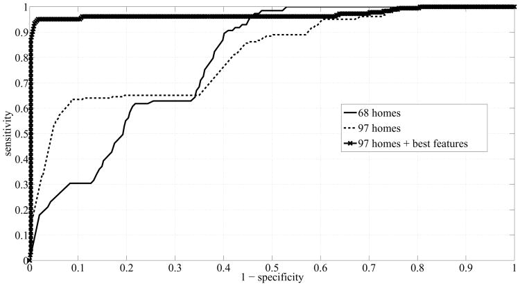
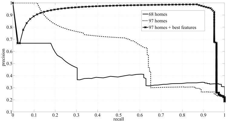
where TP stands for true positives, FN stands for false negatives, TN stands for true negatives, and FP stands for false positives. Since our ROC curves display sensitivity versus (1 - specificity), then an algorithm with good performance yields a point close to the upper left corner of the ROC space, representing a high sensitivity score and a high specificity score. A completely random guess would give a point along the diagonal line from the bottom left corner to the top right corner. Since datasets associated with problems similar to the cognitive status recognition problem at hand are generally biased - having significantly more instances from one class (commonly the negative class) than the other, then using sensitivity and specificity scores only could lead to overly optimistic results. The reason is a system with a biased dataset could yield satisfactory sensitivity and specificity scores but at the same time could be generating too many false positives. In order to address this problem, we also compute precision and recall scores. On a precision versus recall curve, a good performing algorithm would yield a point close to the upper right corner, representing a high average precision (low rate of false positives).

IV. Data, Measures, and Features

All data acquisition was done by ORCATECH who built the first community-wide, home-based assessment platform by deploying sensing technologies in the homes of many older adults and continuously monitoring them unobtrusively for several years.

A. Participants and Data Acquisition

Participants were recruited from the Portland, Oregon, metropolitan area and provided written informed consent before participating in study activities. Eligibility criteria included:

1. being a man or woman aged 80 years or older;

2. living independently in a larger than one-room “studio” apartment;

3. cognitively healthy (Clinical Dementia Rating (CDR) score < 0.5; Mini-Mental State Examination (MMSE) score > 24); and,

4. in average health for age (well-controlled chronic diseases and comorbidities or none at all).

Data were acquired by installing sensing technologies in the homes of the recruited subjects. Subjects' homes ranged from simple one-bedroom apartments with one entry/exit door to houses with as many as 5 bedrooms, a garage, a laundry room, and more than one entry/exit door. Fig. 3 shows an example of a home map with a layout of the sensing technologies. In order to detect movement and general activity by location, passive infra-red motion sensors were installed in rooms frequently visited by the participating subjects, and are represented by the ‘S’ boxes in Fig. 3. Visitors and absences from the home were tracked through wireless contact switches placed on the exit doors of the home, and are represented by the ‘D’ boxes in Fig. 3. Finally, walking speeds were estimated unobtrusively by placing motion sensors on the ceiling approximately 61 cm apart in areas such as a hallway or a corridor, and are represented by the ‘W’ boxes in Fig. 3. These sensors had a restricted field view of ±4° so that they would only fire when someone passed directly under them. A detailed description of how the walking speed was estimated is fully described in [27]. All sensor firings were sent wirelessly to a transceiver, which is represented by the ‘HC’ box in Fig. 3. The firings were time stamped, and then stored in an SQL database. In addition to sensing technologies, recruited subjects were requested to complete a weekly online questionnaire. Using these weekly questionnaires, the subjects reported any visitors during the week, days spent away from the home, any change in health or medication, admittance to ER, and a number of other queries. For further details on data acquisition, the reader is referred to [28] [29].

Fig. 3.

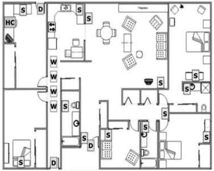
A layout of the sensing technologies that were installed in the homes of the participating subjects [28].

B. Labeling of Data

In this work, we focused only on homes with single occupants, who either remained cognitively intact or transitioned to MCI without bouncing back to cognitive intactness. Occupants were assessed in-home at baseline, and during annual in-home visits by research personnel who administered standardized health and function questionnaires and physical and neurological examinations, including the Mini-Mental State Examination (MMSE) and the Clinical Dementia Rating (CDR). CDR served as our ground truth and was used to determine if subjects were cognitively impaired or intact. A score of 0 on CDR scale indicated cognitive intactness whereas a score of 0.5 on CDR scale indicated mild cognitive impairment. Since subjects were assessed annually, labeling of data fell into three categories:

1. cognitively intact (CIN),

2. unknown (UN), and

3. suffering from MCI (MCI).

The labeling protocol that we implemented in assigning labels to the data is summarized in two examples depicted by Fig. 4 and Fig. 5. Fig. 4 corresponds to a subject who was monitored for a period of more than 3 years and was administered three annual assessments in addition to baseline. The subject scored 0 on CDR scale on all assessments. Therefore, all data from baseline up to the 3rd year assessment were labeled ‘CIN’. Since the subject continued to be monitored after the 3rd year assessment and the 4th year assessment was not available, then any data after the 3rd year assessment were labeled ‘UN’. This was because without the 4th year assessment, it was not possible for us to determine if the subject continued to be cognitively intact or not.

Fig. 4.

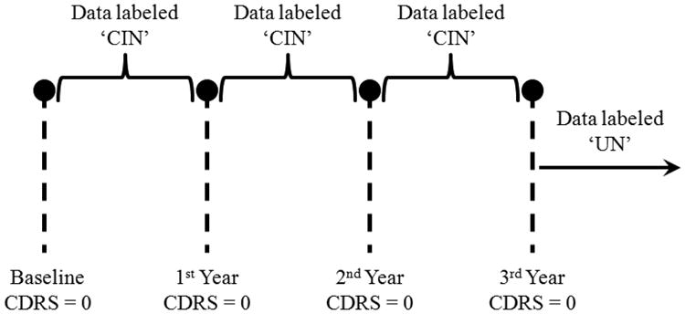
Example of a subject who scored 0 on CDR scale on all administered annual assessments.

Fig. 5.

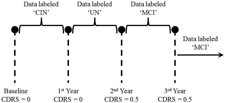
Example of a subject who scored 0.5 on CDR scale on the 2nd-year assessment onward.

Fig. 5, on the other hand, corresponds to a subject who was also monitored for at least 3 years and was administered three annual assessments besides baseline. Unlike the first example, the subject here scored 0 on CDR scale at baseline, but scored 0.5 on CDR scale on the 2nd-year and 3rd-year assessments. Therefore, the data from baseline up to the 1st year assessment were assigned the label ‘CIN’ and the data from the 2nd-year assessment onward were assigned the label ‘MCI’. As for the data between the 1st-year and the 2nd-year assessments, they were assigned the label ‘UN’. This is because the conversion to cognitive impairment is not a point event but a gradual process. Accordingly, the subject's cognitive status would be in flux between years 1 and 2 and would belong to neither cognitive intactness nor MCI.

C. Measures and Features

From the sensor data, a number of predefined measures was computed for each week of monitoring. In order to compute the predefined measures, we made the following definitions:

1. Measures were computed for each week, where a week was defined from Monday to Sunday.

2. Weekly walking speed was computed as the median of all the walking speeds registered within a week.

3. Morning period was defined from 6AM - 3PM, and evening period was defined from 3PM - 12AM.

4. Difference between two variables was computed as the square difference between the medians of the variables, e.g. difference between (x) and (y) was computed as

   $${\mathrm{\Delta }}_{\mathbf{x},\mathbf{y}}={(\mathit{\text{median}}(\mathbf{x})-\mathit{\text{median}}(\mathbf{y}))}^2.$$ (6)

5. A walk was defined as walking under the line of sensors that was used to measure the walking speed.

6. An outing was defined as a firing of any of the exit-doors' sensors followed by a period of inactivity for at least 15 minutes. Exit-doors included front door, back door, garage door, or any other door that the subjects could exit the living unit from.

7. Activity was defined as the total number of sensor firings averaged by the total time spent inside the home.

Based on these definitions, List 1 below presents the measures that were computed:

1. weekly walking speed (ws),

2. coefficient of variation of weekly walking speed (cv_ws),

3. coefficient of variation of weekly morning walking speed (cv_mws),

4. coefficient of variation of weekly evening walking speed (cv_ews),

5. difference between morning and evening speeds (Δ_mes),

6. coefficient of variation of number of walks (cv_w),

7. coefficient of variation of weekly number of outings (cv_o),

8. coefficient of variation of daily activity (cv_da),

9. coefficient of variation of morning activity (cv_ma),

10. coefficient of variation of evening activity (cv_ea), and,

11. difference between morning and evening activities (Δ_mea).

Consequently, the total number of sensor measures, S_m, was equal to 11.

Buracchio et al. recently conducted a study that aimed at comparing the trajectory of motor decline exhibited by older adults who developed MCI and those who remained cognitively intact [30]. Buracchio et al. reported different change points - times at which the change in gait or finger-tapping speed accelerates - between men and women. The study also reported significant difference in baseline gait speed between those who transitioned to MCI and those who did not, only in women. So gender seems to be an important clinical measure to include. Furthermore, it is well-established within the clinical community that age is the most significant known risk factor of dementia. As a result, in addition to the above measures enumerated in List 1, age and gender were included as clinical measures. Accordingly, the total number, R, in (1) was equal to S_m + C_m which was equal to 13, where C_m represented the total number of clinical measures, i.e., 2.

A sliding window of size ℓ was used to extract features from the aforementioned sensor measures. Note that age was computed as the mean age in a window of size ℓ. In this work, we experimented with three types of features:

1. Average of measures, where features were extracted by taking the average of the individual measures in the window of size ℓ. Each w_i,j in (2) was an R-dimensional vector.

2. Probability densities of measures, where features were extracted by estimating the probability densities of the individual measures in the window of size ℓ. By treating each measure as a random variable, we used kernel density estimation to estimate the probability density for each measure using a Normal kernel. These densities were then concatenated into one vector. Accordingly, each w_i,j in (2) was an (S_m × K + C_m)-dimensional vector, where K was the dimension of the probability density, specified based on our discretion.

3. Trajectories of measures, where features were extracted by concatenating the trajectories of the individual measures into one vector. In addition, with this type of features, we kept track of how the walking speed changed within a window by computing the difference between the current walking speed and the window baseline walking speed (Δ_ws,bws), as indicated in Fig. 1. The resulting vector was of length ℓ - 1 since the first entry would always be 0. Accordingly, each w_i,j in (2) was an (S_m × ℓ + ℓ − 1 + C_m)-dimensional vector.

V. Results and Discussion

Of the 97 subjects, 10 were males, 2 of which had MCI at baseline or transitioned to MCI during the monitoring period. The remaining 87 subjects were females, 16 of which had MCI at baseline or transitioned to MCI during the monitoring period. Baseline here corresponds to the beginning of the data that we received from ORCATECH, which for some subjects did not necessarily represent the actual subjects' baseline -when the subjects were recruited. Subjects were monitored for different periods for reasons such as subjects passing away, moving out of the metropolitan area, and subjects withdrawing due to household changes or feeling overwhelmed by study procedures. Table I presents statistics associated with the monitoring periods (in weeks) of the 97 subjects.

Table I. Statistics of monitoring periods of subjects.

monitoring period (in weeks)
minimum	maximum	mean	median	std. deviation
44	260	171.9	186.5	63.7

In this section, we start by describing a preprocessing step that was necessary before we could process the data. Then we report the areas under the curves obtained by executing the cognitive status recognition methodology for the different types of the aforementioned features. Finally, we conclude the section by reporting the best performance after ranking the features in descending order of their importance for detection of MCI.

A. Preprocessing

Because we focused on homes with single occupants, before we could compute the sensor measures presented in List 1, the collected data had to be cleaned. The cleaning process consisted of three main stages:

1. The first stage involved discarding the days on which subjects had their annual assessments. Because assessments were conducted in-home and were administered by research personnel and clinicians, and it was not possible for us to differentiate the research personnel activity from the subjects', these days had to be discarded.

2. The second stage involved discarding the days on which subjects had any visitors over, days which subjects spent away from the home, days spent in ER, days on which subjects had maintenance people over, or days on which people reported health problems that limited their activity.

3. The third stage of cleaning involved discarding days on which sensors failed to fire due to a dead battery or other malfunction.

The most reliable sensors were found to be the motion sensors with the modified field of view, which were used to estimate the subjects' walking speeds. The rest of the sensing technologies were found to be very noisy. Consequently, a large number of days had to be discarded resulting in only 68 homes with sufficient data. Among those 68 subjects, 7 subjects were males, 2 of which had MCI at baseline or transitioned to MCI during the monitoring period. The remaining 61 subjects were females, 13 of which had MCI at baseline or transitioned to MCI during the monitoring period.

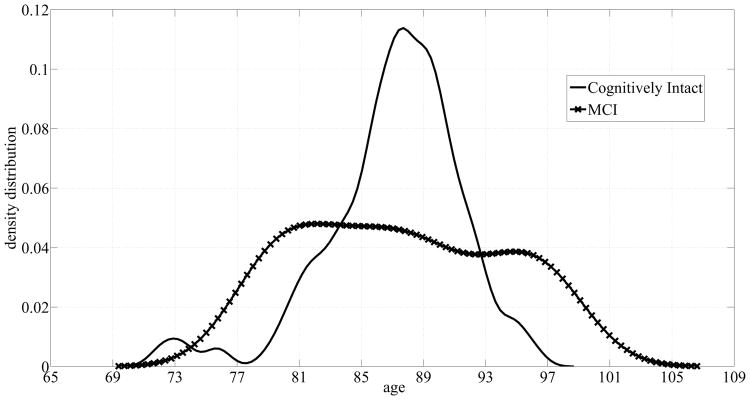
The subjects' age distributions are shown in Fig. 6. Although the cognitively intact subjects' age distribution peaks around 87 to 89 years, the cognitively impaired subjects' distribution covers a wider range of ages resulting in a big overlap between the two groups. As a result, age alone does not suffice in discriminating older adults with MCI.

Fig. 6.

Age probability densities corresponding to the dataset of 68 homes.

B. Implementation Results

Using the cleaned data of the 68 subjects, the measures in List 1 were calculated for each subject and the sets in (1) were generated, and each measure vector was assigned a label as discussed in Section IV. Given that we formulated the cognitive status recognition problem as a classification problem, only the CIN and MCI data were used. In this work, we experimented with two machine learning algorithms: support vector Machines (SVM) and random forests (RF). For implementation of the machine learning algorithms, we used the SVM library, LIBSVM, developed by Chang and Lin [31], to train and test an SVM with a Radial Basis Function (RBF)-kernel. As for RF, we used the TreeBagger class that is part of the Statistics Toolbox in Matlab 2009b. As a baseline model, we trained and test SVM and RF using only age and gender as features. The results are summarized in Table II. Both algorithms performed poorly using only age and gender. This result was expected given the big overlap in the age distributions of the two groups and the gender imbalance of the subjects with a majority of them being females.

Table II.

Baseline model using only age and gender as features for the dataset of 68 subjects.

AUCSS		AUCPR
SVM	RF	SVM	RF
0.47	0.42	0.13	0.10

1) Average of Measures

The first type of features that we experimented with was the average of the individual measures in a window of length ℓ. All the measure vectors as well as the feature vectors were of length 13. Although a dimension of 13 was not considered a high dimension relative to the size of the data, we anticipated that the dimension of the vectors could pose a problem especially with the next two types of features. Accordingly, we decided to introduce a stage of dimensionality reduction alongside with the ‘training and testing’ block in Fig. 2. Principal component analysis (PCA) was chosen to project the data onto a lower dimensional subspace while preserving 95% of the variance in the data. Table III shows the results obtained from trying to recognize the subjects' cognitive status with and without PCA using ℓ = 1 week. The reported results are optimized based on the area under the precision-recall curve, AUC_PR. So the parameters associated with SVM, mainly the soft margin parameter C and the standard deviation of the Gaussian RBF-kernel λ, were optimized to yield the best AUC_PR. Similarly, the parameter associated with RF, mainly the number of trees, was optimized to yield the best AUC_PR. As Table III shows, using PCA led to a 3% increase in AUC_PR with SVM and a 2% increase in AUC_SS. As for RF, using PCA enhanced the algorithm with a 6% increase in AUC_SS and a 2% increase in AUC_PR.

Table III.

Performance of SVM and RF with and without PCA for ℓ = 1 week.

	AUCSS		AUCPR
	SVM	RF	SVM	RF
With PCA	0.68	0.53	0.38	0.13
Without PCA	0.65	0.47	0.33	0.11

Accordingly, all results reported, from this point onward, are based on 3-fold cross validation with each run accompanied by a dimensionality reduction step using PCA and optimized based on AUC_PR.

Table IV provides a summary of the areas obtained by extracting features as the average of the individual measures for ℓ = 1, 2, 3, and 4 weeks. We observe that although AUC_SS was generally more than 0.5 for all ℓ using both algorithms, the algorithms did poorly in terms of AUC_PR. The algorithms were making false positives from 60% to 80% of the time. Also, note that as ℓ increased, the number of datapoints associated with both classes decreased. Finally, although ℓ = 4 weeks yielded the largest AUC_PR using both SVM and PR, an increase in ℓ did not necessarily lead to an increase in the areas under the curves. Intuitively, this was expected because by averaging the measures useful discriminative information could be lost. This gave rise to the second type of features.

Table IV.

Performance of SVM and RF using average of weekly measures for ℓ = 1,2,3, and 4 weeks.

ℓ (in weeks)	Feature Vector Length	# Negative Datapoints	# Positive Datapoints	AUCSS		AUCPR
				SVM	RF	SVM	RF
1	13	3787	482	0.68	0.53	0.38	0.13
2	13	3168	391	0.61	0.56	0.16	0.17
3	13	2689	326	0.41	0.59	0.28	0.16
4	13	2311	278	0.61	0.60	0.43	0.25

2) Probability Densities of Measures

Instead of averaging and potentially losing discriminative information, with the second type of features, we tried to estimate the probability densities of the individual measures in a window of size ℓ. By assuming that each measure was a random variable, we used kernel density estimation to estimate the probability density function that generated the measure samples. The features were represented by the estimated density functions. All density functions were computed at 16 points, resulting in K = 16 for all ℓ and feature vectors of dimension 178 (11 × 16 + 2 = 178) for all ℓ.

Table V presents a summary of the areas under the curves obtained by using features in the form of the probability densities of the measures for ℓ = 4, 8, 12,16, 20, and 24 weeks. The performance of both algorithms in terms of AUC_SS was comparable. In terms of AUC_PR, SVM outperformed RF, especially for smaller ℓ's. However, as Table V shows, the algorithms still performed comparable to a random classifier since AUC_SS obtained using both algorithms was almost equal to 0.5 for all ℓ. With respect to AUC_PR, both algorithms performed worse than a random classifier. As with averaging the measures, the performance of the algorithms did not improve with an increase in ℓ, and the number of datapoints decreased as ℓ increased.

Table V.

Performance of RF and SVM using probability density of measures for ℓ = 4, 8, 12, 16, 20, and 24 weeks.

ℓ (in weeks)	Feature Vector Length	# Negative Datapoints	# Positive Datapoints	AUCSS		AUCPR
				SVM	RF	SVM	RF
4	178	3274	409	0.65	0.45	0.27	0.10
8	178	3368	420	0.56	0.51	0.17	0.12
12	178	3384	410	0.57	0.53	0.26	0.18
16	178	3314	359	0.50	0.41	0.12	0.08
20	178	3262	335	0.49	0.52	0.14	0.13
24	178	3207	311	0.49	0.54	0.14	0.12

3) Trajectories of Measures

We also experimented with features in the form of trajectories of the individual measures as they appeared in a window of size ℓ. One big challenge with this type of features was that the dimension of the data grew with ℓ. Another challenge was that the measure vectors had to exist for all weeks in a given window. If a week was missing, then the whole window of data had to be discarded, and because the sensing technologies were very noisy, a large amount of data ended up being discarded. For a given window of size ℓ, the feature vectors extracted had a dimension of (11ℓ + ℓ - 1 + 2). Table VI presents a summary of the results associated with using features in the form of trajectories of individual measures using ℓ = 4, 8, 12, 16, 20, and 24 weeks.

Table VI.

Performance of SVM and RF using trajectories of individual measures for ℓ = 4, 8, 12, 16, 20, and 24 weeks.

ℓ (in weeks)	Feature Vector Length	# Negative Datapoints	# Positive Datapoints	AUCSS		AUCPR
				SVM	RF	SVM	RF
4	49	2311	278	0.58	0.54	0.35	0.16
8	97	1342	158	0.54	0.46	0.30	0.17
12	145	872	113	0.40	0.38	0.26	0.12
16	193	588	90	0.67	0.51	0.28	0.27
20	241	417	70	0.58	0.50	0.30	0.16
24	289	312	51	0.57	0.49	0.43	0.19

By examining the areas obtained, we found that this type of features yielded the best performance. Similar to the first two types of features, SVM outperformed RF for all ℓ and yielded much higher areas especially in terms of AUC_PR. As expected, as ℓ increased, the number of datapoints associated with each class decreased. Although SVM yielded a promising performance, it was still suffering from a high rate of false positives which was reflected by the low AUC_PR. However, note the high dimension of the data especially for the larger ℓ's, and despite using PCA for dimensionality reduction, the dimension was still high and the poor performance was attributed to the problem of overfitting. With the high dimension, the algorithm learned the training data very well and failed to generalize its learning to data it had not seen before.

4) Speed Measures Only

The sensing technologies were generally very noisy and this had lead to a large amount of data being discarded. However, the lines of sensors which were used to estimate the subjects' walking speeds, were the most reliable and the least noisy. Cleaning data from these sensors only resulted in 97 homes as opposed to 68 homes when all the other sensors were included. Therefore, in order to address the problem of overfitting and by working with the data pertaining to the 68 homes still, we repeated the analysis for recognizing the subjects' cognitive status using only sensor measures associated with the subjects' walking speeds, mainly measures (1 - 6) in List 1 in addition to (Δ_ws,bws) and the clinical measures. Consequently, R from (1) in this case was equal to 9. Since we found that the trajectories of the measures were the best features that yielded the best algorithms' performance, we repeated the analysis using the third type of features only.

Table VII presents a summary of the areas that were obtained for different ℓ. As expected, the dimensions of the feature vectors were greatly reduced to almost half of the original dimensions. Another observation was that, with SVM, AUC_PR increased monotonically with ℓ and the performance of SVM improved by ∼ 20%. As for RF, although the performance was slightly enhanced, it still yielded AUC_PR that was less than 0.5 for all ℓ. This is because RF requires large amounts of data to perform well since it is well-known to be susceptible to overfitting problems. So decreasing the dimension alleviated the overfitting problem and lead to a better performance for both algorithms.

Table VII.

Performance of SVM and RF using trajectories of walking speed measures only.

ℓ (in weeks)	Feature Vector Length	# Negative Datapoints	# Positive Datapoints	AUCSS		AUCPR
				SVM	RF	SVM	RF
4	29	2624	350	0.69	0.71	0.36	0.21
8	57	1541	219	0.69	0.68	0.37	0.24
12	85	997	160	0.70	0.51	0.44	0.15
16	113	673	130	0.67	0.50	0.47	0.17
20	141	474	106	0.68	0.53	0.54	0.24
24	169	349	83	0.79	0.46	0.53	0.21

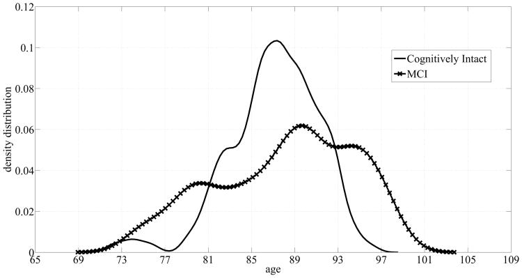
Subsequently, we studied the effect of the data size on the performance of algorithms by using the data pertaining to the 97 homes instead of just 68 homes. So we repeated the analysis for recognizing the subjects' cognitive status using sensor measures (1 - 6) in List 1 in addition to (Δ_ws,bws) and the subjects' age and gender using more data. Fig. 7 displays the age distributions for both classes: cognitive intactness and mild cognitive impairment for the 97 subjects. Adding more subjects did not result in a considerable change in the distribution corresponding to the cognitively intact subjects. On the other hand, the distribution pertaining to the cognitively impaired subjects exhibited a negative skew or was skewed towards older ages. However, there was a still a significant overlap between the two classes, and therefore, using age by itself as a feature does not suffice in detecting older adults with MCI. Similar to the dataset of 68 subjects, we created a baseline model by training and testing SVM and RF on age and gender only. Table VIII shows a summary of the performance of both algorithms. Although both algorithms' performance improved due to the changes in the age distributions, both algorithms still performed poorly, especially in terms of AUC_PR. This supports our observation that age and gender alone do not suffice in discriminating older adults with MCI from their cognitively healthy counterparts.

Fig. 7.

Age probability densities corresponding to the dataset of 97 homes.

Table VIII.

Baseline model using only age and gender as features for the dataset of 97 subjects.

AUCSS		AUCPR
SVM	RF	SVM	RF
0.57	0.54	0.16	0.13

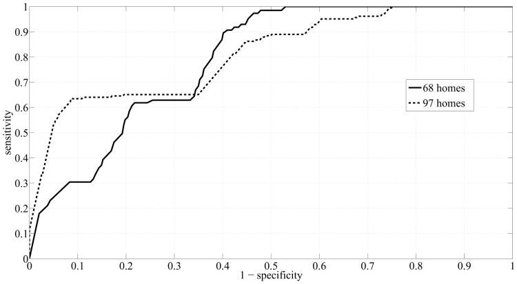
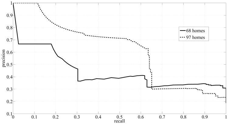
Table IX shows a summary of the areas under the curves that were obtained by using more subjects. A great enhancement was achieved in the performance of RF registering an AUC_SS of 0.8 for ℓ = 12 weeks. However, RF still suffered from a high rate of false positives, reflected as low AUC_PR. On the other hand, SVM yielded very good scores: AUC_SS of 0.81 and AUC_PR of 0.71 for ℓ = 24 weeks, and AUC_PR increased monotonically with ℓ. Fig. 8 and Fig. 9 show the ROC curves and precision-recall curves, respectively, corresponding to SVM with ℓ = 24 weeks, since ℓ = 24 weeks resulted in the best performance. Two curves are potted in each figure. The solid line, shown in Fig. 8, depicts the ROC curve for the case when we used the measures computed from the dataset of 68 homes. The dashed line on the other hand, depicts the ROC curve for the case when we used the measures computed from the dataset of 97 homes. The ROC curve corresponding to the dataset of 97 homes is closer to the top left corner of the figure indicating an enhanced performance in terms of sensitivity and specificity scores. Similarly, Fig. 9 shows the precision-recall curves for both datasets generated by using SVM and ℓ = 24 weeks. Again, the curve corresponding to the dataset of 97 homes exhibited a big shift to the top right corner of the figure indicating an improved performance in terms of precision and recall scores.

Table IX.

Comparison of performance of RF and SVM using trajectories of walking speed measures using the dataset of 97 homes.

ℓ (in weeks)	Feature Vector Length	# Negative Datapoints	# Positive Datapoints	AUCSS		AUCPR
				SVM	RF	SVM	RF
4	29	5093	593	0.70	0.66	0.37	0.16
8	57	3206	408	0.67	0.73	0.53	0.27
12	85	2113	305	0.85	0.79	0.54	0.32
16	113	1477	245	0.80	0.69	0.57	0.32
20	141	1072	211	0.79	0.56	0.62	0.24
24	169	801	183	0.81	0.66	0.71	0.30

Fig. 8.

ROC Curves generated by using SVM and ℓ = 24 weeks.

Fig. 9.

Precision-Recall Curves generated by using SVM and ℓ = 24 weeks.

C. Feature Ranking

After achieving very satisfactory results with SVM and ℓ = 24 weeks, we executed a remove-one-feature process in order to rank the features in terms of their importance for the discrimination process. So we repeated the analysis for recognizing the subjects' cognitive status 9 times and in each time, we removed a feature to see how its absence would affect the overall performance of SVM. Table X presents a summary of the areas that were obtained by removing one feature at a time. The areas obtained when all the features were present served as our reference: AUC_SS = 0.811 and AUC_PR = 0.709.

Table X.

Ranking features by removing one feature at a time using SVM and ℓ = 24 weeks.

Area Under Curve	Feature Removed (in trajectories except for age and gender)
	none	gender	age	Δws,bws	cvw	Δmws,ews	cvews	cvmws	cvws	ws
AUCSS	0.811	0.810	0.781	0.826	0.929	0.812	0.796	0.762	0.751	0.687
AUCPR	0.709	0.599	0.685	0.730	0.779	0.709	0.668	0.656	0.668	0.531

As Table X shows, removing the gender did not have a significant impact on AUC_SS but still lead to a reduction of 10% in AUC_PR indicating an increased rate of false positives. Evidently, gender plays an important role in discriminating older adults with MCI from their cognitively intact counterparts since it accounts for potential sex-specific physiological differences between male and female subjects. As for age, removing it resulted in a reduction of 3% in AUC_SS and a reduction of 2% in AUC_PR. The resulting small change was due to the big overlap between the two classes depicted in Fig. 7. Interestingly, removing Δ_ws,bws and cv_w lead to an enhanced performance with removing cv_w resulting in the best scores. This is most likely because these features were not providing any additional discriminative information. Since we defined SVM with a RBF-kernel, then it would be expected that the algorithm would indirectly learn the difference between the walking speeds and windows' baseline walking speeds. Similarly, cv_w was an indication of the level of activity that the subjects' were exhibiting. Evidently, SVM was able to infer this information from the other features rendering these features unnecessary. Similarly, removing Δ_mws,ews barely resulted in any noticeable change in performance.

The rest of the features that resulted in a deterioration in performance were ws, cv_ws, cv_mws, and cv_ems. Removing trajectories of ws and cv_mws resulted in greater deterioration in terms of AUC_PR compared to removing trajectories of cv_ws and cv_ews. Therefore, variability in walking speed in the morning period was more conducive to detecting older adults with MCI as opposed to variability in the walking speed in the evening period. This potentially is due to the fact that the population of older adults, whether cognitively intact or cognitively impaired, tend to be less active in the evening. Consequently, List 2 below presents the features ranked in descending order of importance:

1. trajectories of weekly walking speed,

2. trajectories of coefficient of variation of morning walking speed,

3. trajectories of coefficient of variation of walking speed,

4. trajectories of coefficient of variation of evening walking speed,

5. age,

6. gender,

7. trajectories of difference between morning and evening walking speeds,

8. trajectories of difference between walking and window baseline speeds, and finally,

9. trajectories of coefficient of variation of number of walks.

By excluding the features that lead to an improved performance when removed, mainly trajectories of Δ_ws,bws, cv_w, and Δ_mws,ews, we repeated the analysis for recognizing the subjects' cognitive status one final time using SVM with ℓ = 24 weeks, and we were able to achieve AUC_SS = 0.97 and AUC_PR = 0.93. The reason for the enhanced performance is that SVM with an RBF kernel is more likely to overfit the data especially with a leave-one-out cross validation process. As mentioned earlier, the removed features did not add additional discriminative information and SVM was most likely able to learn the information provided by these features indirectly from the other features. For example, the difference between the window-baseline walking speed and the current walking speed could be learned from the trajectory of the walking speeds in the window. Therefore, no additional information was added by this feature, and with the high dimension resulting from adding these features, SVM with an RBF-kernel tends to overfit the data, especially when the dimensionality of the feature space is large for the number of data points available. Furthermore, note that removing these features resulted in a tremendous reduction in the dimension of the feature vectors from 169 to 98, which is equivalent to a 42% reduction in dimension, and with the comparatively small data size, a resulting enhancement in performance is expected.

The new ROC curve and the new precision-recall curve are shown in Fig. 10 and Fig. 11 respectively, and compared with the curves that were obtained earlier. The solid lines represent the curves obtained from running SVM on the data from the dataset of 68 homes, the dashed lines represent the curves obtained from running SVM on the data from the dataset of 97 homes, and the lines with x-markers represent the curves obtained from running SVM on the ‘best’ features extracted from the dataset of 97 homes. ‘Best’ refers to features (1 - 6) in List 2. The line with x-markers in Fig. 10 exhibited a big jump towards the top left corner indicating a great improvement in SVM's performance. Similarly, the line with x-markers in Fig. 11 exhibited a big jump towards the top right corner indicating a great improvement in the precision of SVM.

Fig. 10.

ROC Curves corresponding to using SVM for three different cases: dataset of 68 homes, dataset of 97 homes, and dataset of 97 homes + best features.

Fig. 11.

Precision-Recall Curves corresponding to using SVM for three different cases: dataset of 68 homes, dataset of 97 homes, and dataset of 97 homes + best features.

VI. Limitations & Future Work

One limitation of this work is that with features in the form of trajectories of the individuals measures, data have to be present for every week. If a gap exists in the form of a discarded week, then the whole window would be discarded. This poses a serious challenge since older adults are likely to have visitors over more frequently, and with the sensing technologies employed in this study, many weeks could potentially end up being discarded since there is no way to differentiate the activity pertaining to the subjects from the activity pertaining to the visitors. As we have demonstrated, discarding too much data could result in the problem of overfitting, especially for windows of large sizes such as 24 weeks, due to the high dimension of the resulting data.

For future work, we plan to develop proper statistical models of the subjects' activity in their homes and of their walking speeds. In other words, instead of building models based on predefined measures, we plan to build models by processing the raw data itself. We hypothesize that this new approach will be more robust to the problems of missing datapoints and overfitting.

VII. Conclusion

In conclusion, we demonstrated the ability of signal processing along with machine learning algorithms to autonomously detect MCI in older adults. Several measures were calculated from the sensor and clinical data pertaining to 97 homes with single occupants. A sliding time window was then used to generate features to train and test two machine learning algorithms namely SVM and RF. We experimented with different types of features and found that trajectories of the individual measures were the most conducive to discriminating older adults with MCI from their cognitively intact counter parts yielding an area under the ROC curve of 0.81 and an area under the precision-recall curve of 0.71 using SVM. This answered our first research question.

By varying the time window size, mainly from 4 weeks to 24 weeks with a step size of 4 weeks, and by using features in the form of trajectories of measures, we observed a increasing trend in the areas under the curves. The challenge of the high dimension was overcome by adding more data and reducing the number of features. This lead to a great enhancement in the performance of SVM. A time window of size 24 weeks resulted in the highest areas - an area under the ROC curve of 0.81 and an area under the precision-recall curve of 0.71 using SVM. This answered our second research question.

Finally, by carrying out a remove-one-feature process to determine the most important features for detecting older adults with MCI, we found that trajectories of weekly walking speed, coefficient of variation of the walking speed, coefficient of variation of the morning and evening walking speeds, and the subjects' age and gender were the most important for the process of detecting MCI in older adults. Running SVM on these top ranking features autonomously detected MCI in older adults with an area under the ROC curve of 0.97 and an area under the precision-recall curve of 0.93. This answered our third research question.

References

- 1.Senior resource for aging in place. 2011 [Online]. Available: http://www.seniorresource.com/ageinpl.htm.
- 2.Kirby M, LeBreton M. The Health of Canadians - The Federal Role, Volume Two: Current Trends and Future Challenges. 2002 Jan; [Google Scholar]
- 3.Alzheimer society of B.C. 2010 [Online]. Available: http://www.alzheimerbc.org/Get-Involved/Mt--Kilimanjaro---Grouse-Grind-for-Alzheimer-s/The-Cause.aspx.
- 4.Fortinsky R, Wasson J. How do physicians diagnose dementia? Evidence from clinical vignette responses. American Journal of Alzheimer's Disease and Other Dementias. 1997;12(2):51–61. [Google Scholar]
- 5.Clarfield A. The reversible dementias: Do they reverse? Annals of Internal Medicine. 1988;109(6):476–486. doi: 10.7326/0003-4819-109-6-476. [DOI] [PubMed] [Google Scholar]
- 6.Boise L, et al. Diagnosing dementia: Perspectives of primary care physicians. The Gerontologist. 1999;39(4):457–464. doi: 10.1093/geront/39.4.457. [DOI] [PubMed] [Google Scholar]
- 7.Nasreddine ZS, et al. The Montreal Cognitive Assessment (MoCA): A brief screening tool for mild cognitive impairment. J Am Geriatr Soc. 2005;53:695–699. doi: 10.1111/j.1532-5415.2005.53221.x. [DOI] [PubMed] [Google Scholar]
- 8.Folstein MF, et al. “Mini-mental state”: A practical method for grading the cognitive state of patients for the clinician. Journal of Psychiatric Research. 1975;12(3):189–198. doi: 10.1016/0022-3956(75)90026-6. [DOI] [PubMed] [Google Scholar]
- 9.Morris JC. The Clinical Dementia Rating (CDR): Current version and scoring rules. Neurology. 1993;43:2412–2414. doi: 10.1212/wnl.43.11.2412-a. [DOI] [PubMed] [Google Scholar]
- 10.Ganguli M, et al. Detection and management of cognitive impairment in primary care: The steel valley seniors survey. J Am Geriatr Soc. 2004;52(10):1668–1675. doi: 10.1111/j.1532-5415.2004.52459.x. [DOI] [PubMed] [Google Scholar]
- 11.Quinn J, Kaye J. The neurology of aging. The Neurologist. 2001;7:7248–7251. [Google Scholar]
- 12.Hayes TL, et al. Unobtrusive assessment of activity patterns associated with mild cognitive impairment. Alzheimer's and Dementia. 2008;4(6):395–405. doi: 10.1016/j.jalz.2008.07.004. [DOI] [PMC free article] [PubMed] [Google Scholar]
- 13.Monekosso DN, Remagnino P. Behavior analysis for assisted living. IEEE Trans on Automation Science and Engineering. 2010 Oct;7(4):879–886. [Google Scholar]
- 14.Dishman E. Inventing wellness systems for aging in place. Computer. May37(5):34–41. [Google Scholar]
- 15.Barry B, et al. Proc International Symposium on Handheld and Ubiquitous Computing. London, UK: Springer-Verlag; 2000. Easyliving: Technologies for intelligent environments; pp. 12–29. [Google Scholar]
- 16.Helal S, et al. The gator tech smart house: a programmable pervasive space. Computer. 2005 Mar;38(3):50–60. [Google Scholar]
- 17.Abowd G, et al. Proc Conf Human Factors in Computing Systems (CHI) ACM Press; 2000. Living laboratories: The future computing environments group at the Georgia Institute of Technology; pp. 215–216. [Google Scholar]
- 18.Cook DJ. Health monitoring and assistance to support aging in place. J of Universal Computer Science. 2006;12(1):15–29. [Google Scholar]
- 19.GE Healthcare. 2011 [Online]. Available: http://www.careinnovations.com/Data/Downloads/Quietcare/QuietCare_Brochure.pdf.
- 20.Skubic M, et al. Proceedings of the 10th International Smart Homes and Health Telematics Conference on Impact Ananlysis of Solutions for Chronic Disease Prevention and Management, ser ICOST'12. Berlin, Heidelberg: Springer-Verlag; 2012. Testing classifiers for embedded health assessment; pp. 198–205. [Google Scholar]
- 21.Dawadi P, et al. Proceedings of the 2011 workshop on Data mining for medicine and healthcare, ser DMMH '11. New York, NY, USA: ACM; 2011. An approach to cognitive assessment in smart home; pp. 56–59. [Google Scholar]
- 22.Dawadi PN, et al. Automated cognitive health assessment using smart home monitoring of complex tasks. IEEE Transactions on Systems, Man, and Cybernetics. 2013 Nov;43(6):1302–1313. doi: 10.1109/TSMC.2013.2252338. [DOI] [PMC free article] [PubMed] [Google Scholar]
- 23.Dodge HH, et al. In-home walking speeds and variability trajectories associated with mild cognitive impairment. Neurology. 2012 Jun;78(24):1946–1952. doi: 10.1212/WNL.0b013e318259e1de. [DOI] [PMC free article] [PubMed] [Google Scholar]
- 24.Aggarwal NT, et al. Motor dysfunction in mild cognitive impairment and the risk of incident alzheimer disease. Arch Neurolology. 2006;63(12):1763–1769. doi: 10.1001/archneur.63.12.1763. [DOI] [PubMed] [Google Scholar]
- 25.Verghese J, et al. Gait dysfunction in mild cognitive impairment syndromes. J Am Geriatr Soc. 2008;56(7):1244–1251. doi: 10.1111/j.1532-5415.2008.01758.x. [DOI] [PMC free article] [PubMed] [Google Scholar]
- 26.Camicioli R, et al. Motor slowing precedes cognitive impairment in the oldest old. Neurology. 1998;50(5):1496–1498. doi: 10.1212/wnl.50.5.1496. [DOI] [PubMed] [Google Scholar]
- 27.Hagler S, et al. Unobtrusive and ubiquitous in-home monitoring: A methodology for continuous assessment of gait velocity in elders. IEEE Transactions on Biomedical Engineering. 2010;57:813–820. doi: 10.1109/TBME.2009.2036732. [DOI] [PMC free article] [PubMed] [Google Scholar]
- 28.Kaye JA, et al. Intelligent systems for assessing aging changes: Home-based, unobtrusive, and continuous assessment of aging. The Journals of Gerontology Series B: Psychological Sciences and Social Sciences. 2011;66B(suppl 1):i180–i190. doi: 10.1093/geronb/gbq095. [DOI] [PMC free article] [PubMed] [Google Scholar]
- 29.Kaye J, et al. One walk a year to 1000 within a year: continuous in-home unobtrusive gait assessment of older adults. Gait Posture. 2012;35(2):197–202. doi: 10.1016/j.gaitpost.2011.09.006. [DOI] [PMC free article] [PubMed] [Google Scholar]
- 30.Buracchio T, et al. The trajectory of gait speed preceding mild cognitive impairment. Arch Neurology. 2010;67(8):980–986. doi: 10.1001/archneurol.2010.159. [DOI] [PMC free article] [PubMed] [Google Scholar]
- 31.Chang C, Lin C. LIBSVM: a library for support vector machines. 2001 [Online]. Available: http://www.csie.ntu.edu.tw/∼cjlin/libsvm.