Susceptibility-Weighted Imaging and Quantitative Susceptibility Mapping in the Brain

Abstract

Susceptibility-weighted imaging (SWI) is a magnetic resonance imaging (MRI) technique that enhances image contrast by using the susceptibility differences between tissues. It is created by combining both magnitude and phase in the gradient echo data. SWI is sensitive to both paramagnetic and diamagnetic substances which generate different phase shift in MRI data. SWI images can be displayed as a minimum intensity projection that provides high resolution delineation of the cerebral venous architecture, a feature that is not available in other MRI techniques. As such, SWI has been widely applied to diagnose various venous abnormalities. SWI is especially sensitive to deoxygenated blood and intracranial mineral deposition and, for that reason, has been applied to image various pathologies including intracranial hemorrhage, traumatic brain injury, stroke, neoplasm, and multiple sclerosis. SWI, however, does not provide quantitative measures of magnetic susceptibility. This limitation is currently being addressed with the development of quantitative susceptibility mapping (QSM) and susceptibility tensor imaging (STI). While QSM treats susceptibility as isotropic, STI treats susceptibility as generally anisotropic characterized by a tensor quantity. This article reviews the basic principles of SWI, its clinical and research applications, the mechanisms governing brain susceptibility properties, and its practical implementation, with a focus on brain imaging.

TRADITIONALLY, magnetic susceptibility-induced field perturbation is mostly regarded as a source of image artifacts in magnetic resonance imaging (MRI). This treatment is warranted, as no usable soft-tissue contrast is readily available from this perturbation and large field offset creates various unwanted distortions in MRI images. However, magnetic susceptibility is also an intrinsic property of tissue. If treated properly, it can provide important information about tissue structure and function.

Susceptibility-weighted imaging (SWI) is one such technique that takes advantage of the magnetic property to create useful image contrast (1–3). SWI combines a T₂*-weighted magnitude image with a filtered phase image acquired with the gradient echo sequence in a multiplicative relationship (1,3). While the T₂*-weighted magnitude image already provides some susceptibility contrast, SWI further enhances the contrast between tissues of differing susceptibility. In the past decade, SWI has found a growing number of applications in the brain and is being gradually adopted in routine clinical imaging. SWI, however, does not provide quantitative measures of magnetic susceptibility. This limitation is being addressed with the recent development of quantitative susceptibility mapping (QSM) (4–34) and susceptibility tensor imaging (STI) (18,35–46). While SWI generates contrast based on phase images, QSM further computes the underlying susceptibility of each voxel as a scalar quantity. STI, on the other hand, treats susceptibility as a tensor (i.e., a 3 × 3 matrix) quantity rather than a scalar quantity, which allows the quantification of magnetic susceptibility anisotropy (MSA) (35).

The purpose of this review is to provide an overview of the basic principles of susceptibility imaging, the mechanisms governing brain susceptibility properties, corresponding clinical and research applications, and aspects of its practical implementation. All three techniques of SWI, QSM, and STI are reviewed, as they are closely related. Because of the rapid development of these techniques, this limited review cannot exhaustively cover all aspects of the field. Rather, we intend to focus on the basic principles and illustrate their applications with some examples, which can potentially serve a foundation for more in-depth studies.

MAGNETIC SUSCEPTIBILITY AND GRADIENT ECHO

Magnetic susceptibility is a physical quantity that measures the extent to which a material is magnetized by an applied magnetic field. While magnetic susceptibility in general includes both static and AC susceptibility, what is described here is the susceptibility in response to the static B₀ field. Susceptibility of a material, noted by χ, is equal to the ratio of the magnetization, M, within the material to the strength of the applied magnetic field, H, i.e., χ = M/H. In MRI images, this defines the volume susceptibility (dimensionless in SI units). Magnetic materials are classically designated as diamagnetic, paramagnetic, or ferromagnetic. Diamagnetic materials have negative susceptibility while paramagnetic materials have positive susceptibility. Biological tissues can be either diamagnetic or paramagnetic depending on their molecular contents and microstructure. Water, the most abundant molecule in the brain, has a volume susceptibility of −9.035 × 10⁻⁶ (or −9.035 ppm) (SI units) (47), while the variations of susceptibility among brain tissues relative to water is generally small, on the order of ±0.1 ppm (9,10,15,25,48). In comparison, susceptibility of the air is about 0.37 ppm (SI units) (49). Because proton MRI signal is referenced to the Larmor frequency, mainly of water, the field perturbation and frequency shift within the brain are largely due to the significantly different susceptibilities between tissue and air cavities near the brain such as the nasal cavity and ear canals. Contrary to the signal of MRI, which originates from nuclear magnetization, the dominant magnetization that contributes to magnetic susceptibility originates from orbital electrons.

The most commonly used sequence for visualizing the effect of magnetic susceptibility is the spoiled gradient-recalled-echo (SPGR or GRE) sequence (Fig. 1), which can be of a single echo or multiple echoes, 2D or 3D. The magnitude of a series of multiecho GRE images exhibits a single exponential or multiexponential decay (T₂* decay). The phase (Θ) of GRE images measures local frequency offset (f) relative to the Larmor frequency, which reflects the mean magnetic field perturbation seen by spins within a voxel, following the relationship of Θ = −2π ft in a right-hand coordinate system. In this coordinate system, spins with positive gyromagnetic ratio (e.g., protons) rotate clockwise looking down, thus the negative sign (50). The T₂* decay constant is primarily determined by a combination of field inhomogeneities and spin–spin relaxation (T₂). The relationship is typically expressed as R2* = 1/T₂* = 1/T₂ + γΔB/2 or $R_2^{\ast }=R_2+{R^{\prime }}_2$ , where γ is the gyromagnetic ratio, ΔB is the full width at half maximum (FWHM) of the field distribution, and R₂ = 1/T₂.

Figure 1.

A spoiled multiecho gradient echo sequence. Alternating readout polarities are illustrated, although single polarity may also be used. Flow compensation may also be added. The contrast in the magnitude images evolve as the echo time increases due to T₂* decay. Phase values increase as TE increases, thus more phase wraps appear at later echoes. Phase contrast between gray and white matter is still observable under these phase wraps. SWI and QSM may use either single or multiple echoes.

PRINCIPLES OF MAGNETIC SUSCEPTIBILITY IMAGING

Phase Maps of Gradient Echo

The most severe and obvious artifact in the phase of a gradient echo is the discontinuity caused by phase wrapping (Fig. 1). Phase wrapping occurs because sine and cosine functions are periodic with a period of 2π. Any angle outside the range between −π and π will be folded back. In addition, the phase value within the brain is also influenced by the phase of the receiver coils, the long-range magnetic field (dipole field) generated by the human body itself, and the large susceptibility difference between tissue and air. Phase contributed by sources outside a region of interest is commonly referred to as the “background phase.” The presence of large background phase not only disguises local tissue contrast, but also worsens phase wrapping. A common approach in using phase is to perform a phase unwrapping procedure followed by a highpass filtering operation with the assumption that the background phase is smooth, containing only low spatial frequencies (1–3).

A variety of phase unwrapping and background phase removal approaches have been proposed. For example, phase unwrapping can be achieved using conventional path-based methods in the spatial domain and linear fitting methods in the temporal domain (51,52). The difficulty of phase unwrapping can be further compounded by the low signal-to-noise ratio (SNR) (52). The goal of background phase removal is to separate the background phase from phase contributed by brain tissue itself. Traditional highpass filtering, e.g., homodyne filtering, that has been successfully used in SWI, can remove, along with the background phase, a substantial portion of low-frequency components of the tissue phase. This will inevitably lead to inaccurate susceptibility quantification. A number of viable solutions have been developed recently that can more accurately separate background phase from tissue phase. These methods include, for example, the sophisticated harmonic artifact reduction for phase data (SHARP) method and its variants (9,11,28,48), the projection onto dipole fields (PDF) method (53), and harmonic phase removal using the Laplacian operator (HARPERELLA) (23). Particularly, HARPERELLA achieves phase unwrapping and background removal simultaneously.

The value of gradient echo phase was recognized early. For example, Young et al (6) used the field effects to detect changes in tumors, hematomas, lacunar infarct, and multiple sclerosis; Glover (54) used the susceptibility effect to improve the Dixon technique; Conturo et al (55) used the phase to quantify Gd perfusion; filtered phase images also revealed detailed neural anatomy (56,57).

Susceptibility-Weighted Imaging

The central idea of SWI is to enhance susceptibility-induced contrast by combining both magnitude and phase. Magnitude or phase by itself only uses half the acquired information. de Crespigny et al (2) proposed a technique that improved the sensitivity to susceptibility contrast by combining both. They proposed that amplitude and phase could be combined in a number of ways so that they enhanced each other, rather than canceled out and demonstrated one simple approach to reconstruct the real images mag·cos(Θ) after appropriate phase correction to account for various static phase variations.

SWI, as commonly used today (Fig. 2a), was described by Reichenbach et al (3) as “MR Venography.” The main goal was to enhance the visualization of small vessels by taking advantage of the paramagnetic property of deoxyhemoglobin. Cho et al (58) developed a “NMR Venography” that used the susceptibility effect of deoxyhemoglobin. Cho et al relied on the magnitude image generated by a tailored radiofrequency (RF) pulse that suppressed normal tissues while enhancing the signals from blood interfaces, where strong susceptibility-induced fields were present.

Figure 2.

Flowcharts of processing steps of SWI (a) and QSM (b). (a) SWI combines both the magnitude and a filtered phase map in a multiplicative relationship to enhance image contrast. Minimum intensity projection (MIP) is commonly applied to highlight the veins. The contrast can be adjusted by varying the number of slices used in MIP (examples shown in later figures). SWI flowchart adapted from Reichenbach et al (3). (b) There are two major steps involved in QSM: filtering background phase and solving an inverse problem.

The venography technique described by Reichenbach and colleagues was further generalized in the article entitled “Susceptibility weighted imaging” (1). As illustrated in Fig. 2a, in creating SWI, the phase image is highpass-filtered and then transformed to a phase mask that varies in amplitude between zero and one. This mask is multiplied a few times with the original magnitude image to create enhanced contrast between tissues of different susceptibilities. The number of phase mask multiplications can be varied depending on the phase difference and contrast-to-noise ratio, although four multiplications are considered the standard. Haacke et al (1) demonstrated that SWI could be used for enhancing gray matter/white matter (GM/WM) contrast, water/fat contrast, and identifying brain iron, thus extending its application beyond visualizing veins in the brain.

Quantitative Susceptibility Mapping

One intrinsic limitation of signal phase is that phase is nonlocal and orientation-dependent, thus not easily reproducible. For example, the phase of a vein can be either positive or negative depending on its orientation with respect to the B₀ field (59). As a result, the appearance of a vein can vary in SWI images. Furthermore, it is difficult and not always reliable to differentiate diamagnetic susceptibility from paramagnetic susceptibility based on phase or SWI, due to the convoluting effect of the dipole fields. As such, separating calcification which is diamagnetic from iron deposition which is paramagnetic is often challenging in SWI (16). Therefore, it is of great interest to determine the intrinsic property of the tissue, i.e., the magnetic susceptibility, from the measured signal phase (Fig. 2b).

In a simple model where the magnetization of an imaging voxel is treated as a magnetic dipole, each dipole will produce a magnetic field (dipole field) that spatially extends beyond that voxel itself (Fig. 3a). The magnetic field at any given voxel is thus a superposition of all dipole fields generated by surrounding voxels. Because the superposition of magnetic field is linear and the field of a unit dipole is shift invariant (i.e., it does not change from one voxel to another), the relationship between the spatial distribution of susceptibility (which is proportional to magnetization) and the spatial distribution of frequency (which is proportional to magnetic field) is governed by a simple convolution. The impulse response function is the unit dipole field. Convolution in the image domain can be also expressed as multiplication in the k-space (13,14):

$$f(\mathbf{k})=\mathrm{\gamma }{B}_0(\frac{1}{3}-\frac{k_z^2}{k^2})\mathrm{\chi }(\mathbf{k})$$ [1]

Figure 3.

Relationship between susceptibility and magnetic field. (a) Each image voxel can be approximated as a magnetic dipole which produces a dipole field that extends beyond the voxel itself. Dipole fields originating from different voxels follow the superposition rule resulting in a convolution relationship between field and susceptibility which can be expressed as a multiplication in the k-space. (b) Solving the inverse problem from field to susceptibility is ill-posed, as the coefficients of the equation become zero on a surface of cone in the k-space when k² = 3k²_z.

Here, k is the k-space vector and k_z is its z-component; f(k) is the Fourier transform of the map of frequency offsets f(r); B₀ is the magnetic flux density corresponding to the applied magnetic field H₀ in vaccum; χ(k) is the Fourier transform of the susceptibility distribution χ(r); γ is gyromagnetic ratio. Note that only the z-component of the susceptibility-induced field perturbation is measurable in the frequency shift.

Mapping susceptibility requires solving the linear equation shown in Eq. (1) where f(k) is the experimental measurement and χ(k) is the unknown. Inverting Eq. (1) is problematic when k₂ = 3k²_z (a conical surface in k-space) as the coefficient becomes zero (Fig. 3b). Consequently, χ(k) cannot be accurately determined in regions near the conical surfaces. A variety of approaches have been proposed to address this issue. These techniques are generally called quantitative susceptibility mapping (QSM). A number of QSM algorithms have been developed (4–15). There are software packages now available for research purposes, for example, MEDI (12) and STI Suite (23). As a convention, all susceptibility maps will be displayed with brighter intensity representing paramagnetic susceptibility and dark intensity representing diamagnetic susceptibility (Fig. 3). One exception is when visualizing susceptibility anisotropy of white matter, in which case the intensity scale is flipped (Fig. 4).

Figure 4.

Examples of magnetic susceptibility anisotropy and STI in the brain. (a,c) Susceptibility maps measured at three orientations of a mouse brain at 9.4T (a) and a human brain at 3T (c). The values and contrast of the white matter are clearly orientation dependent. Notice that intensity scale is flipped with diamagnetic susceptibility appearing bright. (b,d) Corresponding color-coded eigenvector maps calculated by STI. Imaging parameters at 9.4T are: 3D SPGR, matrix size = 256 × 256 × 256, FOV = 22 × 22 × 22 mm³, flip angle = 60°, TE = 8 msec, and TR = 100 msec, 19 orientations. Parameters at 3T are: flow-compensated 3D SPGR, TE = 40 msec, TR = 60 msec, flip angle = 20°, FOV = 256 × 256 × 256 mm², matrix size = 128 × 128 × 128, 16 orientations.

Susceptibility Tensor Imaging

Equation (1) assumes that magnetic susceptibility is isotropic and a scalar quantity; in other words, susceptibility shall not vary with respect to the relative orientation between B₀ and the brain. However, recent studies found that susceptibility of brain white matter is in fact anisotropic (Fig. 4a,c). Liu (35) found extensive anisotropic magnetic susceptibility in the white matter of intact mouse brains while Lee et al (41) showed anisotropic susceptibility in excised segments of human brain corpus callosum. A susceptibility tensor imaging (STI) technique was proposed to measure and quantify this phenomenon (35). This technique relies on the measurement of frequency offsets at different orientations with respect to the main magnetic field. The orientation dependence of susceptibility is characterized by a tensor. In the brain’s frame of reference, the relationship between frequency shift and susceptibility tensor is given by (35):

$$f(\mathbf{k})=\mathrm{\gamma }{B}_0\left(\frac{1}{3}{\widehat{\mathbf{H}}}^{\mathrm{T}}\mathbf{\chi }(\mathbf{k})\widehat{\mathbf{H}}-\widehat{\mathbf{H}}·\mathbf{k}\frac{{\mathbf{k}}^{\mathbf{T}}\mathbf{\chi }(\mathbf{k})\widehat{\mathbf{H}}}{k^2}\right)$$ [2]

Here, χ is a second-order (or rank-2) susceptibility tensor; Ĥ is the unit vector (unitless) of the applied magnetic field. Assuming that the susceptibility tensor is symmetric, then there are six independent variables to be determined for each tensor. In principle, a minimum of six independent measurements are necessary. A set of independent measurements can be obtained by rotating the imaging object, e.g., tilting the head, with respect to the main magnetic field. Given a set of such measurements, a susceptibility tensor can be estimated by inverting the system of linear equations formed by Eq. (2). Fewer than six orientations are also feasible by incorporating fiber orientation estimated by diffusion tensor imaging (DTI) and assuming cylindrical symmetry of the susceptibility tensor (36,39).

The susceptibility tensor can be decomposed into three eigenvalues (principal susceptibilities) and associated eigenvectors (Fig. 4b,d). Similar to DTI fiber tractography, fiber tracts can be reconstructed based on STI (38,40). The main challenge of STI is the requirement of rotating the brain inside the MR scanner. To overcome this challenge, Liu and Li (60) showed that the higher-order frequency variations based on a single image acquisition without rotating the object could provide sufficient information to probe the white matter architecture. With the advances of ultrahigh field MRI systems and more accurate and in-depth understanding of GRE phase, it is anticipated that GRE phase will become a powerful tool for studying the microstructures of the brain.

MECHANISMS OF SUSCEPTIBILITY CONTRAST

There are several factors affecting the volume susceptibility measured by MRI. On the atomic level, paramagnetic susceptibility originates from spins of unpaired electrons which have a higher tendency to align with an applied magnetic field and amplify the field. Diamagnetic susceptibility, on the other hand, originates from the induction currents of circulating electrons that generate fields opposing the applied field. On the molecular level, the availability of unpaired electrons, the distribution of electron cloud within the molecule, and the competition between electron spins and induction currents will together determine the molecule’s susceptibility and anisotropy. Finally, the microstructure of the brain tissue, i.e., the spatial arrangement of molecules and organelles within a voxel, will affect the microscopic magnetic field distribution within the voxel. As the water molecules are distributed within this heterogeneous magnetic field environment, what MRI phase measures is the averaged effect as seen by these molecules. As a result, the distribution (e.g., compartmentalization) and motion of the water molecules affect the perceived phase shift. In a healthy adult brain, the most striking feature of phase and susceptibility maps are that the gray matter largely appears paramagnetic and the white matter largely diamagnetic (5,9,48). The emerging consensus is that the paramagnetic susceptibility of gray matter is mainly related to iron and the diamagnetic susceptibility of white matter is due to myelination.

Brain Iron

While iron is ferromagnetic and iron is present in the human body, no known human tissues are actually ferromagnetic. In human beings, iron is mostly stored in ferritin and hemosiderin; both are paramagnetic (Table 1). In the brain, certain regions have a preferential accumulation of nonheme iron. Hallgren and Sourander (61) studied the distribution of iron in eighty-one brains at autopsy. They found a progressive increase in iron distribution that plateaus in the late teens or twenties with a second, milder increase after age 60, which they fitted to an exponential growth function. Recent QSM studies largely agree that the paramagnetic susceptibility of deep brain nuclei is predominately due to iron deposition (10,11,57). Postmortem MRI and mass spectrometry have validated that susceptibility measured by QSM is linearly correlated with iron concentration in the deep brain nuclei (62). It has thus been proposed that QSM can be a potential in vivo means for quantifying brain iron stores. The study by Li et al (24) evaluated susceptibility as a function of age in a cohort of 191 healthy participants from 1 to 83 years of age (Fig. 5). The results indicated that magnetic susceptibility of iron-rich gray matter nuclei followed an exponential growth trajectory, which confirmed the findings by Hallgren and Sourander (61).

Table 1.

Magnetic Susceptibility of Common Biomolecules Encountered in SWI and QSM

Materials	Volume susc.1 (SI, unitless) χv, ppm	Molar Susc.2 (CGS, cm3/mol, emu/mol) χm, ppm	Conditions and references	Areas of relevance
Water (H2O)	−9.035	−12.98	20°C, Arrighini et al (47).
Hydroxyapatite (Ca2+)	−14.83		Room temperature; measured by NMR; χv = −1.18 in CGS. Hopkins and Wehrli (111).	Vascular calcification, Tumor
Phospholipid	χ̄ = −9.68	χ̄ = −5803	20°C, magneto-orientation method, phospholipid DPPC. Kawamura et al (63); phospholipid composes of stearic acids.	Myelination demyelination dysmyelination Multiple sclerosis
	χ|| = −10.43	χ|| = −6303
	χ⊥ = −9.30	χ⊥ = −560
	χa = −1.13	χa = −683
Stearic acid CH3(CH2)16COOH	χ̄ = −10.03	χ̄ = −218.4	20°C, Gouy method, powder stearic acid. ρ = 1.04 g/cm3, molar mass M = 284.4772 g/mol. Lonsdale 1939 (64).
	χ1 = −9.65	χ1 = −210.0
	χ2 = −10.83	χ2 = −235.7
	χ3 = −9.56	χ3 = −208.2
	χa = −1.22	χa = −26.6
Oxyhemoglobin (HbO2, Fe3+)4		−893	20°C, Gouy method. Pauling and Coryell (90); Coryell et al (91).	BOLD fMRI Cerebral vascular diseases
Deoxyhemoglobin (Hb, Fe2+)		11,910	25°C, Gouy method, Taylor and Coryell (92).
Methemoglobin (Hb+, Fe3+)		14,000	24°C, Gouy method, in solution, per heme. Coryell et al (91).	Methemoglobinemia Sickle cell disease
Hemosiderin (Fe2+ and Fe3+)		4,810	22°C, Gouy method, thick suspension. Michaelis et el (94).	Hemorrhage Hemochromatosis
Ferritin (Fe3+)		6,132	22°C, Gouy method, in solution, per heme. Michaelis et el (94).	Brain iron stores Mitochondrial disease Neurodegeneration
Ceruloplasmin (Cu2+)		550	20°C, susceptometer balance, in solution, Ehrenberg et al (108).	Wilson’s disease

Shaded volume susceptibility values were converted from reported experimental molar susceptibility values (unshaded) in the relevant literature. Not all values were converted due to the unknown sample mass density and molar mass at the time of the reported experiments. The molar susceptibilities of phospholipid and oxyhemoglobin are much larger than that of water because of the presence of many more contributing chemical bonds within a molecule, see, e.g., Lonsdale (64).

¹Magnetic susceptibility values are reported in the literature based on several different definitions (volume, mass, and molar susceptibility) and units (SI, CGS, CGS emu). Significant variations exist due to variations in measurement techniques and sample preparations.

²Conversion from molar to volume susceptibility follows ${\mathrm{\chi }}_v={\mathrm{\chi }}_m\frac{\mathrm{\rho }}{M}$ where ρ is the mass density (g/cm ³) and M is the molar mass (g/mol). Conversion from CGS to SI units follows χ_v (SI) = 4πχ_v (CGS).

³Mean susceptibility χ̄ = (χ₁ + χ₂ + χ₃)/3; parallel susceptibility χ_|| is the susceptibility along the long axis of the carbon chain; susceptibility anisotropy is χ_a = χ₂ − (χ₁ + χ₃)/2 or χ_a = χ_|| − χ_⊥.

⁴There are still debates on the iron state in oxyhemoglobin.

Figure 5.

QSM of brain development and aging. (a) Susceptibility values and contrast evolve as a function of age. Brain nuclei become more paramagnetic (hyperintense) as the age increases. Gray and white matter contrast also increases overall. (b) Susceptibility is diamagnetic in the white matter. It first decreases, becoming more diamagnetic during brain development and maturation, followed by an increase as the brain ages. (c) In the nuclei, susceptibility increases monotonically following an exponential function of age. IC, internal capsule; OR, optical radiation; GP, globus pallidus. The scan parameters are: in-plane resolution = 0.9 × 0.9 mm², matrix = 256 × 208, flip angle = 20°, TE of first echo = 4.92 msec, echo spacing = 4.92 msec, TR = 35 msec, and number of echoes = 6. The slice thickness is 2 mm.

On the other hand, the lowest iron concentrations were found in the cerebral and cerebellar hemispheric white and gray matter (61). Hallgren and Sourander (61) also reported that the subcortical “U” fibers had greater iron content than either the cerebral gray or white matter. In addition, the frontal white matter had a greater iron distribution than the occipital white matter, with almost no ferric iron in the most posterior portion of the posterior limb of the internal capsules and optic radiations. In high-resolution phase maps acquired at 7T, Duyn et al (57) observed a strong paramagnetic frequency shift in layer IV of the cortex which was attributed to high iron concentration in the cell body. However, when iron was extracted from postmortem tissues, the strong phase and susceptibility contrast between cortical gray and white matter did not change significantly (62). This is because the susceptibility of the white matter is predominantly determined by myelin.

Myelin

In the phase and susceptibility maps of the brain, white matter consistently shows diamagnetic susceptibility. It is now clear that this diamagnetic susceptibility is due to the presence of myelin. Myelin is a spiraling sheath that wraps around nerves, including those in the brain and spinal cord. It is made up of proteins and lipids that provide electric insulation. Most proteins and lipids have diamagnetic susceptibility. For example, phospholipids have a mean molar susceptibility of −580 cm³/mol (CGS units) and are anisotropic (Table 1) (63,64). The volume susceptibility of phospholipids is also slightly more diamagnetic than water (Table 1). The purpose of the myelin sheath is to allow action potentials to transmit quickly and efficiently along the axons of nerve cells. Myelin is essential for the proper functioning of the nervous system. Loss of the myelin sheath is the hallmark of a number of neurodegenerative autoimmune diseases including multiple sclerosis. The importance of myelin in forming the diamagnetism and susceptibility anisotropy has been demonstrated in a number of studies. In one study, it was shown that the strong susceptibility contrast between white and gray matter disappeared in the transgenic dysmyelinating shiverer mouse whose myelin did not develop properly (65). The phase contrast also decreased when mice were fed with a cuprizone diet that resulted in demyelination in the central nervous system (66).

Myelination is also an age-dependent process. Both human and rodent brains are poorly or not myelinated at birth. Myelination occurs rapidly in the first few years of life for human and in the first few weeks for rodents. On the other hand, demyelination occurs as the brain ages. In human neonates, it was shown that phase contrast was reduced (67). In the developing mouse brain from postnatal day 4 (PND4) to PND40, it was also observed that phase contrast between gray and white matter correlated with the optical intensity of myelin stained histological slides (68). However, both studies were based on phase contrast rather than the more intrinsic tissue susceptibility value. In a recent QSM study of 191 participants from 1 to 83 years of age, it was further revealed that susceptibility of white matter first became more diamagnetic as the brain developed, followed by a continuing decrease in diamagnetism as the brain aged (24) (Fig. 5). This developmental trajectory was explained by the myelination and demyelination process which occurred in normal brain development and aging. In the mouse brain, Argyridis et al (20) evaluated the temporal evolution of magnetic susceptibility in the white matter of mouse C57BL/6 from PND2 to PND56. They confirmed that susceptibility became increasingly diamagnetic as the brain developed. More interestingly, they also found that susceptibility anisotropy increased monotonically as a function of age; there was a sign change for susceptibility in the white matter around the third week, and diamagnetic susceptibility was highly correlated with myelin staining intensity (R² = 0.93).

Microstructure

Besides its chemical and molecular composition, brain tissue’s microstructure (cellular and subcellular structures and arrangement of cells) also play a crucial role in affecting the MRI-measured susceptibility. Compartmentalization of white matter (e.g., separation of axonal space, myelin space, and extracellular space) plays a significant role in affecting the phase and T₂* signal behavior (18,42,69,70). Protons in each compartment experience unique magnetic field and relaxation properties. The effect of microstructure can be generalized into two categories: orientation dependence and distribution of subvoxel magnetic field. These effects are especially prominent in the white matter due to its unique microstructure that cannot be treated as homogeneous even in a statistical sense.

Orientation effects include the angular dependence of magnetic fields generated by elongated structures (71) and the angular dependence due to underlying anisotropic susceptibility (35,41). For simplicity, we will refer to the former as “structural anisotropy” and the latter as “susceptibility anisotropy.” Structural anisotropy can generate orientation-dependent phase even with only isotropic susceptibility simply due to the geometric shape. A classic example is the field shift of a vessel inside the magnet which is dependent on the relative angle between the vessel and the field (59). In an analysis of gray-white matter phase contrast, He and Yablonskiy (71) predicted a dependence of white matter phase on the relative angle between axons and magnetic field due to the elongated shape of the axons similar to the vessels.

Susceptibility anisotropy describes that magnetic susceptibility is a tensor quantity rather than a scalar quantity (35). As a result, the interaction between susceptibility and magnetic field follows the rule of tensor-vector product rather than a simple scaling effect. In brain tissues, especially in the white matter, this anisotropy originates mainly from membrane lipids (37). Each lipid molecule has an anisotropic response to an external magnetic field due to its chain-like structure and nonspherical distribution of electron clouds. Li et al (37) demonstrated that it was the anisotropic susceptibility of lipid molecules and the ordered arrangement of these lipids that gave rise to the bulk susceptibility anisotropy observed on the voxel level. Wharton and Bowtell (42) simulated the field distribution within myelinated axons by modeling axons as hollow cylinders. They concluded that anisotropic susceptibility of myelin was needed to fully explain the behavior of the GRE phase.

For a given imaging voxel containing heterogeneous structures, magnetic field within the voxel is also heterogeneous, while the total magnetization of the voxel is a summation of all spins within the voxel, each experiencing a slightly different local magnetic field. The phase angle of the resulting signal represents the strength of the mean field. The spatial heterogeneity, however, is lost during the ensemble averaging. Liu and Li proposed a spectral analysis technique in the Fourier spectrum space (p-space) that could recover the field distribution within the voxel thus allowed them to infer the underlying tissue microstructure (60). Specifically, this method measures the spatial variation of the magnetic field within a voxel that is induced by the underlying structural heterogeneity. The underlying principle is that, in the direction parallel to the axons, the field variation is expected to be minimal, while the variation is the largest in the directions perpendicular to the axons. The ability to detect such spatial variations is enhanced at higher field strengths due to the increased susceptibility effect.

Other Sources

There are a number of other sources that affect GRE phase contrast in the brain. In the blood pool, oxygenation changes hemoglobin from being paramagnetic (deoxyhemoglobin) to being diamagnetic (oxyhemoglobin) (Table 1). This change of magnetic property is essential for visualizing veins with SWI and is the basic mechanism underlying blood oxygenation level-dependent (BOLD) functional MRI (fMRI) (72). However, hemoglobin does not play any significant role in affecting the susceptibility contrast between gray and white matter (73). Chemical exchange between mobile protons and proteins does affect the phase contrast between gray and white matter and it decreases the susceptibility-induced contrast (74).

While the effect of calcium on phase and susceptibility contrast in healthy brain tissues has not been fully investigated, calcification in diseased tissues such as tumors causes the local tissue to appear diamagnetic (16). This shift is the opposite of that caused by iron deposition. Schweser et al (16), for example, used this diamagnetic property to delineate calcified lesions, vessels, and potentially iron-laden tissue. They showed that discrimination of para- from diamagnetic lesions was possible and the results were confirmed by the additional computed tomography (CT) in one patient.

CLINICAL AND RESEARCH APPLICATIONS

SWI is now commonly used in clinical neuroimaging, while applications of susceptibility mapping techniques are still primarily in the research stage. Reflecting the contrast mechanisms outlined in the previous section, the applications of these techniques generally involve changes of substances in the brain that exhibit different magnetic susceptibility compared to the surrounding tissues and structures.

SWI of Cerebral Vascular Pathology

A key application of SWI is aiding the diagnosis of diseases involving cerebral vascular pathology. These changes include, for example, vascular malformations (e.g., arteriovenous malformations and cerebral cavernous malformations), restrictions in blood flow (e.g., developmental venous anomaly) and hemorrhages (caused by e.g., cerebral amyloid angiopathy, stroke, and traumatic injuries) (1,3,75–89). In these cases, a common source of contrast is oxygenation-related susceptibility changes occurring in blood products (3). The main blood oxygen carrier, hemoglobin, contains a heme molecule with an Fe²⁺ atom. Due to the binding with oxygen, oxyhemoglobin has no unpaired electrons; its susceptibility is determined by the protein shell and thus is diamagnetic (90,91) (Table 1). Deoxyhemoglobin, on the other hand, has four unpaired electrons per heme and is paramagnetic (90,92) (Table 1). Deoxyhemoglobin can be further oxidized to methemoglobin (ferrihemoglobin) which contains an Fe³⁺ per heme with five unpaired electrons (91) (Table 1). Although methemoglobin has low concentration in normal blood, its concentration increases following hemorrhage, but the effect is mostly manifested as T₁-shortening rather than susceptibility effects (91,93). In the final stages, after hemorrhage, hemosiderin often forms when macrophages phagocytose and degrade the extracellular hemoglobin; hemosiderin is also paramagnetic (94) (Table 1).

Arteriovenous malformations (AVM) is one example of vascular malformation which consists of arteriovenous shunt with branches off the internal carotid artery (ICA) and cerebral veins. Small AVMs may be occult on CT angiography (CTA) or MRA, yet be readily identified on SWI (75). Although small, these AVMs can hemorrhage and thus are not clinically insignificant. Figure 6 illustrates one example of hemorrhage from AVM in an 8-year-old boy whose positive susceptibility enhancement can be verified by QSM (Fig. 6b). In addition, effects associated with AVM other than hemorrhage are also visible on SWI (75,95): for example, intravascular hyperintensity near AVM may suggest oxygenated blood due to rapid arteriovenous shunting and rapid flow to the varix via the AVM; hyperintensity of parenchyma may suggest edema due to the T₂ effect of AVM-related venous hypertension or AVM-related steal phenomenon; on the other hand, hypointensity may suggest prolonged time passage of normal intracranial blood, venous engorgement, or possible functional obstruction caused by the AVM.

Figure 6.

An 8-year-old boy with hemorrhage from an ateriovenous malformation. (a) CT obtained at presentation showed right frontal lobe hemorrhage (arrow). (b) QSM obtained at 3T shortly after the CT showed bright signal abnormality, confirming the presence of iron/hemorrhage (arrow). Additional areas of curvilinear and nodular bright signal was seen medial to the lesion, possibly suggesting additional areas of hemorrhage, thromboses, or abnormal vasculature or draining vein containing deoxyhemoglobin (arrowhead). GRE sequence parameters are: 3D multiecho EPI, flip angle 20°, 1 × 1 × 1 mm³, BW 62.50 kHz, TR = 59.3 msec, TE = 13, 28, 43 msec. (c) SWI minIP image demonstrated abnormal vascular tangle typical of arteriovenous malformation (arrow). (d) Final diagnosis of arteriovenous malformation was confirmed by cerebral angiogram.

Developmental venous anomaly (DVA) is one example of low flow vascular anomalies that is particularly well demonstrated by SWI (96,97). DVAs consist of a radially oriented array of aberrant veins that converge into a single larger venous stalk. These are often occult on noncontrasted MR images, but are readily detected on SWI (96). Figure 7 shows an example of a large cerebellar DVA in a 5-year-old boy with prominent draining. DVAs have an association with another type of low flow vascular anomaly: the cerebral cavernous malformation (CCM) which, unlike DVAs, is at risk for hemorrhage. The identification of a DVA on an imaging study can, therefore, indicate the need to intensify the search for CCMs.

Figure 7.

A 5-year-old boy presented with a large cerebellar developmental venous anomaly (DVA). (a) Multiple linear, branching low signal abnormality is seen in the left cerebellum on SWI minIP image, suggestive of DVA (arrow). Low signal abnormality in the brainstem associated with enhancement (not shown) representing telangiectasia (arrowhead) is also noted. (b) Cerebral angiogram confirmed characteristic feature of DVA in this patient, including a large draining venous stalk (arrow). (c) QSM also identifies dominant draining venous stalk (arrowhead) and multiple anomalies veins (arrows) as bright signal, likely due to presence of deoxyhemoglobin. SWI/QSM protocol is the same as Fig. 6.

Cerebral cavernous malformations (CCM) is another example of low-flow vascular malformations that are composed of dilated thin-walled capillaries. CCM has a propensity to hemorrhage, thus the detection of cavernous malformations is not trivial. If a CCM has previously bled, it is often clearly visible on routine MRI or CT images. SWI can be confirmatory in these situations, displaying low signal related to extravasated blood products. The CCMs that have not previously hemorrhaged, especially the small ones, are a particular challenge on conventional imaging modalities because they are often quite subtle. SWI, on the other hand, is sensitive to CCMs regardless of the presence of prior hemorrhage (96) (Fig. 8). In a study evaluating patients with known familial CCM lesions, de Souza et al (98) found that SWI outperformed both T₂ fast spin echo (FSE) and T₂* gradient echo (GRE) sequences in terms of identifying more lesions throughout the brain.

Figure 8.

SWI is very sensitive to slow flow vascular malformations such as cerebral cavernous malformations (CCM), as in this child with a large left temporal CCM (dashed arrows), with a characteristic “popcorn” appearance on CT and MRI. There are typical internal calcifications on CT (a), hyperintense subacute blood products on T₁WI (b), mild internal enhancement on postcontrast T₁WI (c), and peripheral hypointense hemosiderin on FLAIR (d) and T₂WI (e). The lesion appears larger on SWI (f) due to blooming artifact. More important, additional smaller CCMS are detected (solid arrows), which indicate that the patient likely has multiple familial CCM syndrome (which can occur in as many as 1/3 of patients with CCM). SWI parameters are: 3T, TE = 20 msec, TR = 29 msec, FA = 15°, FOV 250 mm × 188 mm, matrix 448 × 336, 2 mm thick acquisition displayed with 16 mm minIP.

Cerebral Amyloid Angiopathy (CAA) has a classic presentation of a lobar cerebral hemorrhage, typically in an elderly patient. The deposition of beta amyloid protein within the arteriolar wall is thought to result in an inflammatory response leading to vessel wall fragility and local ischemia. On SWI, the patient will have numerous microhemorrhages (<10 mm in diameter, also known as cerebral microbleeds), appearing as foci of hypointensity, predominantly within the cerebral cortex or near the gray–white junction (99) (Fig. 9). In order to suggest this diagnosis, microhemorrhages must be visible in a typical distribution, generally within the cerebral cortex near the gray–white junction (99).

Figure 9.

SWI can play an important role in diagnosing cerebral amyloid angiopathy (CAA) and changing patient management. Microbleeds in CAA are in contrast to those from chronic hypertension, which are typically located in the deeper structures such as the deep white matter, deep gray nuclei, or brainstem. These microbleeds were not visible on any other imaging sequence or modality. These patients are at risk for intracranial hemorrhage and should avoid anticoagulation therapy. (a) Numerous tiny microbleeds are seen on SWI, scattered throughout the cortex of the cerebral hemispheres (white arrows) in this elderly patient, typical for CAA. These lesions are also well visualized on maximum intensity projection of QSM (b) and filtered phase maps (c). Projection was made through 8 slices each of 2-mm thickness. Note that the small veins are shown most clearly on the SWI image, less clearly on the phase, and even less so on the QSM projection. Imaging parameters are: 1.5T, TE = 35ms, TR = 85ms, 512 × 512 × 64 acquisition matrix, BW = 160 Hz/pixel, ETL = 5, FA = 25° and acquisition time roughly 8 minutes. (a–c) Courtesy of Saifeng Liu and E. Mark Haacke. (d–f) A 73-year-old patient presented with progressive encephalopathy. SWI shows numerous microbleeds in a cortical pattern (solid arrows), likely due to cerebral amyloid angiopathy (CAA). Patchy edema was also present (dashed arrows), suggestive of CAA-related inflammation. (d–f) Image parameters were: 1.5 T, TE = 40 msec, TR = 57 msec, FA = 20°, FOV 256 × 256, matrix 512 × 512, 2 mm thick acquisition, and 16 mm thick minimal intensity projection.

Ischemic and hemorrhagic stroke can both be visualized by SWI. In acute infarctions, SWI is more sensitive than CT or T₂* GRE for the detection of hemorrhage, a finding that would preclude the patient from undergoing thrombolysis (79). Following thrombolysis, SWI has been found to be able to detect hemorrhagic transformation earlier than CT (76). Perfusion-weighted imaging combined with diffusion-weighted imaging has shown considerable promise for identifying the ischemic penumbra (Fig. 10). When the levels of blood deoxyhemoglobin rise due to increased oxygen extraction, the degree of “blooming” artifact within the veins increases. Some have proposed that this finding can be used in a manner similar to the penumbra of MR perfusion images, detailing areas of the brain that are potentially salvageable. One study by Baik et al (100) illustrated this concept, as prominent veins were noted in the hypoperfused region. This finding resolved following restoration of arterial flow, presumably due to normalization of the oxygen extraction fraction in the tissues and thus a reduction in venous deoxyhemoglobin.

Figure 10.

SWI can provide important information in the setting of stroke, as in this 50-year-old male who presented with acute dissection and occlusion of the right internal carotid artery in the neck. Diffusion-weighted image (a) showed a small infarct in the right frontal white matter (dashed white arrow) Parametric map of mean transit time, from dynamic-contrast enhanced MR perfusion (b) showed a large area of delayed perfusion (large white arrows) in the right MCA territory, demarcating a large penumbra. SWI image at the level of the circle of Willis (c) showed abnormal hypointense signal in the right MCA (open white arrow) compared to the normal hyperintense signal in the left MCA (open black arrow), indicating slow flow or intravascular thrombus or markedly elevated intra-arterial deoxyhemoglobin. SWI image at the level of the lateral ventricles (d) showed markedly prominent cortical and deep medullary veins in the right hemisphere (small solid white arrows), matching the penumbra. The prominent veins indicate high levels of deoxyhemoglobin, indicating increased oxygen extraction. SWI parameters are: 3T, TE = 20 msec, TR = 29 msec, FA = 15°, FOV 230 mm × 172 mm, matrix 448 × 336, 2 mm thick acquisition displayed with 16 mm minIP.

Traumatic brain injury (TBI) may result in extraaxial hemorrhages that are easily detectable by CT or conventional MRI. Some patients, however, have more subtle or occult injuries. SWI is proving to be of diagnostic and likely prognostic value in the evaluation of TBI patients (77,101–104) (Fig. 11). SWI has repeatedly outperformed T₂*-weighted images, detecting up to six times as many lesions in one head-to-head comparison (77). There are a number of patients, primarily those with diffuse axonal injury, whose neurological deficits are not adequately explained by the extent of pathology visible on CT (103). Pathological studies have shown that, along with injuring the myelin sheaths and axons, shearing forces at the time of trauma can injure the small vessels accompanying the neurons, resulting in microhemorrhages (105). Note that not all axonal injuries lead to microhemorrhages; however, those with a hemorrhagic component have been suggested to indicate a more severe injury and a poorer prognosis (106).

Figure 11.

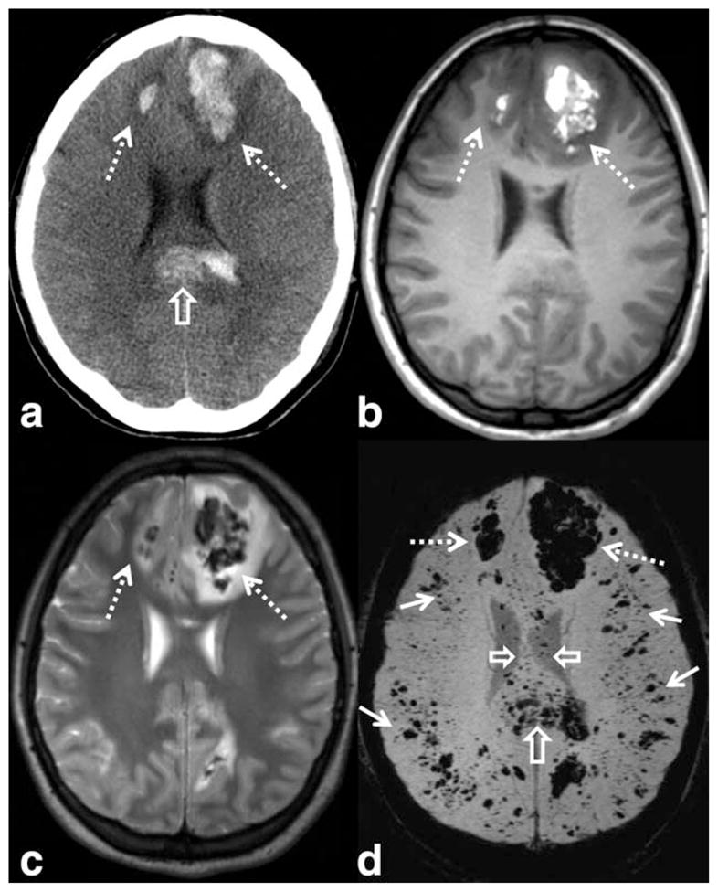
SWI has shown higher sensitivity to traumatic microhemorrhages, particularly in the setting of diffuse axonal injury. Images from a young patient involved in a motor vehicle accident shows large hemorrhagic contusions in the frontal lobes (dashed arrows) on CT (a), T₁-WI (b), T₂-WI (c), and SWI (d). A large hemorrhagic shearing injury in the corpus callosum is also visible on CT, but more extensive involvement is visible on SWI (open arrows). Widespread traumatic microhemorrhages throughout the gray–white matter junction are only visible on SWI (solid white arrows). SWI parameters are: 3T, TE = 20 msec, TR = 29 msec, FA = 15°, FOV 250 mm × 188 mm, matrix 448 × 336, 2 mm thick acquisition displayed with 16 mm minIP.

SWI of Mineral Deposition

Abnormal mineral deposition exists in many neurological diseases. SWI is sensitive for detecting abnormal accumulation of molecules containing minerals including, for example, iron, copper, and calcium. In the brain parenchyma, iron is mostly stored in ferritin as Fe³⁺ (ferric) in a crystalline solid form and in hemosiderin, which contains both ferritin and cell debris. Each ferritin can store up to about 4500 Fe³⁺ ions and is highly paramagnetic (94) (Table 1). In human, the majority of the body’s copper is in the Cu²⁺ form (107), with 90% of total plasma copper stored in paramagnetic blue protein ceruloplasmin (108) (Table 1); copper proteins in the brain parenchyma, however, have not been fully identified (109). While calcium is normally stored in the skeleton, pathological calcification may also occur in tumor and vessel wall (110). In skeleton bone, calcium phosphate mineral aligns with the structured cellular tissue and with the periodicity of negative charges on collagen. The characteristic mineral of bone is hydroxyapatite, whose susceptibility value is sparsely reported in the literature. In one study, Hopkins and Wehrli (111) measured the susceptibility of hydroxyapatite to be −14.82 ppm SI units (or −1.18 ppm in CGS units), slightly more diamagnetic than water (Table 1).

Abnormal iron deposition, in a group of phenotypically similar disorders collectively known as Neurodegeneration with Brain Iron Accumulation, involves the subcortical gray matter including the basal ganglia, thalamus, substantia nigra, and dentate nucleus (112). Abnormal iron metabolism has also been implicated in a number of other brain diseases and disorders including Parkinson’s disease, Alzheimer’s disease, and multiple sclerosis (113,114). Because of the paramagnetic susceptibility of iron binding proteins, SWI and QSM have been applied in studying these and other related diseases (115,116). It was recently reported that 3D multiecho SWI of the sub-stantia nigra at 7T may be used to accurately differentiate healthy subjects from PD patients (117).

Wilson’s disease (WD), on the other hand, is due to an abnormality in copper metabolism with the end result being excessive copper accumulation, particularly in the subcortical gray matter structures (globus pallidus, putamen, thalamus, dentate nucleus, pons, and midbrain) (118). In a study with 23 WD subjects and 23 controls, Bai et al (119) found significant negative phase values in the subcortical gray matter. Fritzsch et al (120), using QSM, showed that patients with WD had significantly increased susceptibility in all analyzed basal ganglia regions compared with healthy controls, which was evident not only in patients with a neurological syndrome but also in patients with isolated hepatic manifestations.

Applications of Susceptibility Mapping

Although the diagnostic value of QSM still needs to be fully investigated, the quantitative information has already shed additional light on brain development, aging, and the evolution of pathologies. One immediate potential clinical utility of QSM is to improve the localization and quantification of calcium with MRI, which can be differentiated from microbleeds and iron deposition due to the diamagnetic nature of calcification (Table 1) (16) (Fig. 12). In one study, QSM provided more accurate differentiation of calcifications from hemorrhage (21). One benefit of establishing an MRI-based method for detecting calcification is to reduce radiation exposure to vulnerable pediatric patients.

Figure 12.

QSM can differentiate calcification from iron deposit and veins. (a,b) An elderly volunteer shows numerous hypointense spots in the thalamus (solid arrows) and in the ventricles (dotted arrows) adjacent to veins and choroid plexus on T₂*-weighted images (a). QSM (b) reveals hypointense calcifications (dotted arrows) in the ventricles which are clearly differentiated from the adjacent veins and iron deposition in the thalamus. (c–f) An 8-month-old male infant with tuberous sclerosis and multiple calcified dysplasias and hamartomas. (c) Numerous cortical/subcortical tubers, or dysplasias, (arrowhead) and subependymal nodules (arrows) were seen on the T₂ FSE image. (d) Corresponding QSM image revealed dark signal associated with many of these lesions, which would be expected for calcification but not iron (arrows and arrowhead). SWI/QSM protocol of (c,d) is the same as Fig. 6. (e,f) This was confirmed by CT.

In multiple sclerosis (MS) patients, SWI allows the visualization of the anatomic relationship of the demyelinating plaque and the penetrating veins (121,122). In one study, combining conventional imaging sequences with SWI demonstrated ~50% more lesions than did the conventional sequences alone, including those in the cortical gray matter that were often difficult to visualize on fluid-attenuated inversion recovery (FLAIR) (115). While demyelination is the hallmark of MS, elevated iron deposits have also been reported in MS brains (123,124). Both demyelination and iron deposition increase local tissue susceptibility which can be quantified by QSM (Fig. 13), although differentiating their relative contributions remains a topic of research. It has been shown that loss of myelin causes the susceptibility of white matter to increase (i.e., becoming less diamagnetic), approaching that of gray matter (65,66). At the same time, demyelination reduces R2* while iron deposition increases R2*. These competing effects on R2* have been thought to result in the improved sensitivity of QSM over R2* in evaluating changes in the basal ganglia of MS patients (22). Further, QSM of MS lesions at various ages showed that lesions’ susceptibility increased rapidly as it changed from being enhanced to nonenhanced; during the first few years, lesions attained a high susceptibility value and gradually dissipated back to susceptibility similar to that of normal-appearing white matter as the lesions aged (34).

Figure 13.

A 49-year-old multiple sclerosis patient. (a) MS plaques are usually best visualized on FLAIR images. (b) Hyperintense lesions on FLAIR may exhibit increased magnetic susceptibility on the QSM images (arrows). The sizes and boundaries of hyperintense lesions appear differently on QSM. This increased susceptibility may indicate demyelination and or iron deposition. (c) SWI without minIP shows the perivenular distribution of the lesions and venous involvement. SWI and QSM may provide greater understanding of the pathophysiology of the disease. SWI/QSM parameters are: in-plane resolution = 0.9 × 0.9 mm², matrix = 256 × 208, flip angle = 20°, TE of first echo = 4.92 msec, echo spacing = 4.92 msec, TR = 35 msec, and number of echoes = 6. The slice thickness is 2 mm. [Color figure can be viewed in the online issue, which is available at wileyonlinelibrary.com.]

The quantitative nature of QSM offers an opportunity to correlate susceptibility values with clinical conditions and treatment outcomes. In a recent study of β-thalassemia, a blood disorder that reduces the production of hemoglobin, in 31 patients who had been under blood transfusion treatment, 27 (87.1%) had abnormal iron deposition in one of the regions of interest (ROIs) examined. Compared with healthy control subjects, patients with thalassemia showed significantly lower susceptibility value in the globus pallidus and sub-stantia nigra but significantly higher susceptibility value in the red nucleus and choroid plexus (125). QSM should also be relevant for evaluating the effect of chelation on brain iron in other diseases such as sickle cell disease and Parkinson’s disease.

QSM is also being applied to quantify cerebral perfusion, as susceptibility changes in the blood can be directly related to the concentration of gadolinium-based contrast agent (33) or endogenous deoxyhemoglobin (126,127). The theoretical advantage of QSM as opposed to T₂*-weighted images is to provide a more accurate estimate of tissue perfusion without suffering from “blooming” artifacts. Because of its sensitivity to deoxyhemoglobin, QSM allows the mapping of the source of the BOLD contrast in gradient echo fMRI (128,129). In one recent study at 7T, it was reported that the sensitivity and spatial reliability of functional QSM relative to the magnitude data depended strongly on the significance threshold that defines “activated” voxels in the SPM software, and on the efficiency of spatiotemporal filtering of the phase time-series (32). For high-resolution 7T data, the observed phase and susceptibility changes in the cortex have been attributed to blood volume and oxygenation changes in pial and intracortical veins (129).

STI is being developed as a high-resolution fiber-tracking technique. Its feasibility has been demonstrated on mouse brains (38). Improved tracing of renal tubules has been recently demonstrated with STI and it was shown that STI was able to track tubules throughout the kidney, whereas DTI was limited to the inner medulla in mouse kidneys (40). Further developments are underway for applications in human brains (36,39,43). There is growing evidence suggesting that QSM and susceptibility anisotropy may be a sensitive measure for loss of myelin in brain white matter (20,65,66,68,130). Cao et al (130) recently reported that prenatal alcohol exposure significantly reduces susceptibility contrast and susceptibility anisotropy of the brain white matter, and magnetic susceptibility may be more sensitive than DTI for detecting subtle myelination changes.

IMPLEMENTATIONS AND UNMET NEEDS

Technical Considerations

Most, if not all, modern MRI scanners are readily equipped with some versions of the 2D and 3D gradient echo sequence. This type of sequence is known to be fast, robust, and of low specific absorption rate (SAR). At 3T, a typical scan duration is around 5–10 minutes, depending on the spatial resolution and slice coverage. The sequence can be optimized with respect to field strength, flip angle, TE, TR, and the tissue and pathology of interest (Table 2). A key requirement during acquisition is to store the complex images (both magnitude and phase) rather than only the magnitude. For QSM, the orientation of the B₀ field needs to be known with respect to the imaging matrix.

Table 2.

Examples of SWI and QSM Protocols for the Brain

Field	Recon	Resolution (mm3)	Flip angle	TE1 (msec)	TR (msec)	# echo
1.5 T	SWI	0.8 × 0.8 × 2	20°	40	50	1
	QSM	0.8 × 0.8 × 2	30°	Min	58	Multi
3.0 T	SWI	0.8 × 0.8 × 2	15°	20	28	1
	QSM	0.8 × 0.8 × 2	12°	Min	40	Multi
7.0 T	SWI	0.3 × 0.3 × 1.2	15°	15	28	1
	QSM	0.8 × 0.8 × 0.8	8°	Min	34	Multi

These sequence parameters are not intended as general “recommendations.” Rather, they serve to illustrate parameter examples that produce good SWI and QSM results. The parameters should be modified for different purposes; for example, multiple echoes can also be acquired for SWI.

SNR

A “rule of thumb” for SNR consideration is that optimal phase SNR is attained at TE = T₂* for a given type of tissue (131). If the primary purpose is to visualize veins and hemorrhages such as in SWI venography, the TE can be chosen to be around 20 msec at 3T; if the purpose is to visualize gray and white matter contrast with QSM, better SNR is achieved with the TE around 30–40 msec at 3T. Both SWI and QSM benefit from increasing field strength, as phase accumulates faster at higher field, allowing shorter TE and TR, thus less T₂* decay, higher SNR, and more rapid acquisition.

Contrast

Since SWI combines both magnitude and phase, contrast in the magnitude image affects the appearance of SWI (1). For example, low flip angles and intermediate TEs result in low gray matter and white matter contrast; a slightly higher flip angle partially suppresses the cerebrospinal fluid (CSF) and adds some T₁-weighting. QSM, on the other hand, is not sensitive to magnitude contrast except for the potential multi-compartment effect, where relative contributions from different compartments may vary depending on sequence parameters.

2D vs. 3D

While SWI can be reconstructed from both 2D and 3D data, susceptibility mapping is best accomplished with a 3D sequence to avoid phase inconsistency among adjacent slices, although 2D data are also compatible with QSM (32,132). For 2D acquisition, a single echo with interleaving slices allows fast volume coverage, which is beneficial for dynamic scans such as perfusion and functional QSM. For 3D acquisitions, multiple echoes offer the flexibility of optimizing SWI contrast (133,134) and improving SNR for QSM through multiecho averaging (131). Fast acquisition can also be achieved with spiral or EPI trajectories for both 2D and 3D acquisitions (131,132).

High readout bandwidth (> 62 kHz) and high spatial resolution are beneficial for QSM in reducing intravoxel dephasing and subsequent signal loss. Finally, flow compensation is useful for suppressing phase accumulation due to arterial blood and bulk motion (62,127,135).

For image reconstruction, some MRI manufacturers provide commercial software to generate SWI images on the scanner. There are also shared research software packages now available for susceptibility mapping (12,23).

Unmet Needs and Future Directions

A growing number of algorithms have been proposed for QSM, most of which are developed based on limited simulation, phantom, and in vivo data. There is a lack of systematic evaluation and critical comparisons of the accuracy, intersubject variability, and intrasubject reproducibility. A rigorous assessment of the performances of the algorithms and the dependence on pulse sequences can potentially lead to an acceptable standard for MRI susceptibility mapping and facilitate its clinical translation. Such an assessment should include sequence parameters, phase unwrapping, background phase removal, and susceptibility inversion algorithms. Establishing such a standard will require concerted efforts across multiple centers and different vendors.

A critical obstacle in interpreting susceptibility values is the competing effects of multiple signal sources. While the susceptibility of white matter is predominantly determined by myelin concentration, iron is also present, e.g., in oligodendrocyte that forms the myelin and in mitochondria in the axons (136). On the other hand, while the susceptibility of deep brain nuclei is mostly determined by iron deposition, axons within these nuclei are also myelinated, although to a lesser degree. In pathological tissues such as MS plaques, demyelination and iron deposition may coexist. In Wilson’s disease, copper deposition may also be accompanied by iron accumulation (137). While QSM provides a quantification of the susceptibility values, it is unable to differentiate these diverse sources of susceptibility by itself. Patient history, clinical symptoms, other MRI parameters, sophisticated signal models, and possibly other imaging modalities are thus needed to pinpoint the exact cause of detected alterations in susceptibility.

Characterizing and imaging subvoxel magnetic field distribution is another emerging area of interest, which may provide insight into tissue microstructure. The volume susceptibility measured by QSM reflects only the mean field shift of a given voxel, it does not portray the field heterogeneity within the voxel. A basic model for this field heterogeneity is the three-pool model of axonal water, myelin water, and extracellular water (42,69). A more systematic way to extract the subvoxel field information is to perform a Fourier spectral analysis with the p-space technique which has been demonstrated in phantoms and mouse brains ex vivo (60). Another way is to measure diffusion attenuation caused by this internal heterogeneous magnetic field (138,139).

In conclusion, While susceptibility is a major source of image artifacts in MRI, technological advances have also transformed it into a useful source of image contrast. SWI is gaining wider acceptance in clinical practice. Susceptibility mapping techniques aim to quantify the underlying sources. However, it is acknowledged that QSM provides only a “relative” quantification of susceptibility rather than the absolute physical quantity. This is because MRI phase and frequency values are relative and are also affected by phase filtering procedures, and there is a lack of universal and reliable frequency reference for in vivo imaging. The clinical application of susceptibility mapping is still in the early stage of evaluation. The immediate goals are to image and quantify many biologically and pathologically relevant endogenous molecules, exogenous contrast agents, and tissue microstructures and their relationships with disease diagnosis and prognosis.

References

- 1.Haacke EM, Xu Y, Cheng YC, Reichenbach JR. Susceptibility weighted imaging (SWI) Magn Reson Med. 2004;52:612–618. doi: 10.1002/mrm.20198. [DOI] [PubMed] [Google Scholar]
- 2.de Crespigny AJ, Roberts TP, Kucharcyzk J, Moseley ME. Improved sensitivity to magnetic susceptibility contrast. Magn Reson Med. 1993;30:135–137. doi: 10.1002/mrm.1910300121. [DOI] [PubMed] [Google Scholar]
- 3.Reichenbach JR, Venkatesan R, Schillinger DJ, Kido DK, Haacke EM. Small vessels in the human brain: MR venography with deoxyhemoglobin as an intrinsic contrast agent. Radiology. 1997;204:272–277. doi: 10.1148/radiology.204.1.9205259. [DOI] [PubMed] [Google Scholar]
- 4.de Rochefort L, Brown R, Prince MR, Wang Y. Quantitative MR susceptibility mapping using piece-wise constant regularized inversion of the magnetic field. Magn Reson Med. 2008;60:1003–1009. doi: 10.1002/mrm.21710. [DOI] [PubMed] [Google Scholar]
- 5.Shmueli K, de Zwart JA, van Gelderen P, Li TQ, Dodd SJ, Duyn JH. Magnetic susceptibility mapping of brain tissue in vivo using MRI phase data. Magn Reson Med. 2009;62:1510–1522. doi: 10.1002/mrm.22135. [DOI] [PMC free article] [PubMed] [Google Scholar]
- 6.Young IR, Khenia S, Thomas DG, et al. Clinical magnetic susceptibility mapping of the brain. J Comput Assist Tomogr. 1987;11:2–6. doi: 10.1097/00004728-198701000-00002. [DOI] [PubMed] [Google Scholar]
- 7.Weisskoff RM, Kiihne S. MRI susceptometry: image-based measurement of absolute susceptibility of MR contrast agents and human blood. Magn Reson Med. 1992;24:375–383. doi: 10.1002/mrm.1910240219. [DOI] [PubMed] [Google Scholar]
- 8.Li L. Magnetic susceptibility quantification for arbitrarily shaped objects in inhomogeneous fields. Magn Reson Med. 2001;46:907–916. doi: 10.1002/mrm.1276. [DOI] [PubMed] [Google Scholar]
- 9.Li W, Wu B, Liu C. Quantitative susceptibility mapping of human brain reflects spatial variation in tissue composition. Neuroimage. 2011;55:1645–1656. doi: 10.1016/j.neuroimage.2010.11.088. [DOI] [PMC free article] [PubMed] [Google Scholar]
- 10.Bilgic B, Pfefferbaum A, Rohlfing T, Sullivan EV, Adalsteinsson E. MRI estimates of brain iron concentration in normal aging using quantitative susceptibility mapping. Neuroimage. 2012;59:2625–2635. doi: 10.1016/j.neuroimage.2011.08.077. [DOI] [PMC free article] [PubMed] [Google Scholar]
- 11.Wu B, Li W, Guidon A, Liu C. Whole brain susceptibility mapping using compressed sensing. Magn Reson Med. 2012;67:137–147. doi: 10.1002/mrm.23000. [DOI] [PMC free article] [PubMed] [Google Scholar]
- 12.Liu J, Liu T, de Rochefort L, et al. Morphology enabled dipole inversion for quantitative susceptibility mapping using structural consistency between the magnitude image and the susceptibility map. Neuroimage. 2012;59:2560–2568. doi: 10.1016/j.neuroimage.2011.08.082. [DOI] [PMC free article] [PubMed] [Google Scholar]
- 13.Marques JP, Bowtell R. Application of a Fourier-based method for rapid calculation of field inhomogeneity due to spatial variation of magnetic susceptibility. Concept Magn Reson B. 2005;25B:65–78. [Google Scholar]
- 14.Salomir RDSB, Moonen CTW. A fast calculation method for magnetic field inhomogeneity due to an arbitrary distribution of bulk susceptibility. Concepts Magn Reson Part B. 2003;19B:26–34. [Google Scholar]
- 15.Wharton S, Bowtell R. Whole-brain susceptibility mapping at high field: a comparison of multiple- and single-orientation methods. Neuroimage. 2010;53:515–525. doi: 10.1016/j.neuroimage.2010.06.070. [DOI] [PubMed] [Google Scholar]
- 16.Schweser F, Deistung A, Lehr BW, Reichenbach JR. Differentiation between diamagnetic and paramagnetic cerebral lesions based on magnetic susceptibility mapping. Med Phys. 2010;37:5165–5178. doi: 10.1118/1.3481505. [DOI] [PubMed] [Google Scholar]
- 17.Tang J, Liu S, Neelavalli J, Cheng YCN, Buch S, Haacke EM. Improving susceptibility mapping using a threshold-based k-space/image domain iterative reconstruction approach. Magn Reson Med. 2013;69:1396–1407. doi: 10.1002/mrm.24384. [DOI] [PMC free article] [PubMed] [Google Scholar]
- 18.Dibb R, Li W, Cofer W, Liu C. Microstructural origins of gadolinium-enhanced susceptibility contrast and anisotropy. Magn Reson Med. 2014 doi: 10.1002/mrm.25082. Epub ahead of print. [DOI] [PMC free article] [PubMed] [Google Scholar]
- 19.Acosta-Cabronero J, Williams GB, Cardenas-Blanco A, Arnold RJ, Lupson V, Nestor PJ. In vivo quantitative susceptibility mapping (QSM) in Alzheimer’s disease. PLoS One. 2013;8:e81093. doi: 10.1371/journal.pone.0081093. [DOI] [PMC free article] [PubMed] [Google Scholar]
- 20.Argyridis I, Li W, Johnson GA, Liu C. Quantitative magnetic susceptibility of the developing mouse brain reveals microstructural changes in the white matter. Neuroimage. 2013 doi: 10.1016/j.neuroimage.2013.11.026. Epub ahead of print. [DOI] [PMC free article] [PubMed] [Google Scholar]
- 21.Deistung A, Schweser F, Wiestler B, et al. Quantitative susceptibility mapping differentiates between blood depositions and calcifications in patients with glioblastoma. PLoS One. 2013;8:e57924. doi: 10.1371/journal.pone.0057924. [DOI] [PMC free article] [PubMed] [Google Scholar]
- 22.Langkammer C, Liu T, Khalil M, et al. Quantitative susceptibility mapping in multiple sclerosis. Radiology. 2013;267:551–559. doi: 10.1148/radiol.12120707. [DOI] [PMC free article] [PubMed] [Google Scholar]
- 23.Li W, Avram AV, Wu B, Xiao X, Liu C. Integrated Laplacian-based phase unwrapping and background phase removal for quantitative susceptibility mapping. NMR Biomed. 2013 doi: 10.1002/nbm.3056. Epub ahead of print. [DOI] [PMC free article] [PubMed] [Google Scholar]
- 24.Li W, Wu B, Batrachenko A, et al. Differential developmental trajectories of magnetic susceptibility in human brain gray and white matter over the lifespan. Hum Brain Mapp. 2013 doi: 10.1002/hbm.22360. Epub ahead of print. [DOI] [PMC free article] [PubMed] [Google Scholar]
- 25.Lim IA, Faria AV, Li X, et al. Human brain atlas for automated region of interest selection in quantitative susceptibility mapping: application to determine iron content in deep gray matter structures. Neuroimage. 2013;82C:449–469. doi: 10.1016/j.neuroimage.2013.05.127. [DOI] [PMC free article] [PubMed] [Google Scholar]
- 26.Liu T, Wisnieff C, Lou M, Chen W, Spincemaille P, Wang Y. Nonlinear formulation of the magnetic field to source relationship for robust quantitative susceptibility mapping. Magn Reson Med. 2013;69:467–476. doi: 10.1002/mrm.24272. [DOI] [PubMed] [Google Scholar]
- 27.Schweser F, Deistung A, Sommer K, Reichenbach JR. Toward online reconstruction of quantitative susceptibility maps: super-fast dipole inversion. Magn Reson Med. 2013;69:1582–1594. doi: 10.1002/mrm.24405. [DOI] [PubMed] [Google Scholar]
- 28.Sun H, Wilman AH. Background field removal using spherical mean value filtering and Tikhonov regularization. Magn Reson Med. 2013 doi: 10.1002/mrm.24765. Epub ahead of print. [DOI] [PubMed] [Google Scholar]
- 29.Wang S, Lou M, Liu T, Cui D, Chen X, Wang Y. Hematoma volume measurement in gradient echo MRI using quantitative susceptibility mapping. Stroke. 2013;44:2315–2317. doi: 10.1161/STROKEAHA.113.001638. [DOI] [PMC free article] [PubMed] [Google Scholar]
- 30.Xie L, Sparks MA, Li W, et al. Quantitative susceptibility mapping of kidney inflammation and fibrosis in type 1 angiotensin receptor-deficient mice. NMR Biomed. 2013;26:1853–1863. doi: 10.1002/nbm.3039. [DOI] [PMC free article] [PubMed] [Google Scholar]
- 31.Zheng W, Nichol H, Liu S, Cheng YC, Haacke EM. Measuring iron in the brain using quantitative susceptibility mapping and X-ray fluorescence imaging. Neuroimage. 2013;78:68–74. doi: 10.1016/j.neuroimage.2013.04.022. [DOI] [PMC free article] [PubMed] [Google Scholar]
- 32.Balla DZ, Sanchez-Panchuelo RM, Wharton SJ, et al. Functional quantitative susceptibility mapping (fQSM) Neuroimage. 2014;100:112–124. doi: 10.1016/j.neuroimage.2014.06.011. [DOI] [PubMed] [Google Scholar]
- 33.Bonekamp D, Barker PB, Leigh R, van Zijl PC, Li X. Susceptibility-based analysis of dynamic gadolinium bolus perfusion MRI. Magn Reson Med. 2014 doi: 10.1002/mrm.25144. Epub ahead of print. [DOI] [PMC free article] [PubMed] [Google Scholar]
- 34.Chen W, Gauthier SA, Gupta A, et al. Quantitative susceptibility mapping of multiple sclerosis lesions at various ages. Radiology. 2014;271:183–192. doi: 10.1148/radiol.13130353. [DOI] [PMC free article] [PubMed] [Google Scholar]
- 35.Liu C. Susceptibility tensor imaging. Magn Reson Med. 2010;63:1471–1477. doi: 10.1002/mrm.22482. [DOI] [PMC free article] [PubMed] [Google Scholar]
- 36.Li X, Vikram DS, Lim IA, Jones CK, Farrell JA, van Zijl PC. Mapping magnetic susceptibility anisotropies of white matter in vivo in the human brain at 7 T. Neuroimage. 2012;62:314–330. doi: 10.1016/j.neuroimage.2012.04.042. [DOI] [PMC free article] [PubMed] [Google Scholar]
- 37.Li W, Wu B, Avram AV, Liu C. Magnetic susceptibility anisotropy of human brain in vivo and its molecular underpinnings. Neuroimage. 2012;59:2088–2097. doi: 10.1016/j.neuroimage.2011.10.038. [DOI] [PMC free article] [PubMed] [Google Scholar]
- 38.Liu C, Li W, Wu B, Jiang Y, Johnson GA. 3D fiber tractography with susceptibility tensor imaging. Neuroimage. 2012;59:1290–1298. doi: 10.1016/j.neuroimage.2011.07.096. [DOI] [PMC free article] [PubMed] [Google Scholar]
- 39.Wisnieff C, Liu T, Spincemaille P, Wang S, Zhou D, Wang Y. Magnetic susceptibility anisotropy: cylindrical symmetry from macroscopically ordered anisotropic molecules and accuracy of MRI measurements using few orientations. Neuroimage. 2013;70:363–376. doi: 10.1016/j.neuroimage.2012.12.050. [DOI] [PMC free article] [PubMed] [Google Scholar]
- 40.Xie L, Dibb R, Cofer GP, et al. Susceptibility tensor imaging of the kidney and its microstructural underpinnings. Magn Reson Med. 2014 doi: 10.1002/mrm.25219. Epub ahead of print. [DOI] [PMC free article] [PubMed] [Google Scholar]
- 41.Lee J, Shmueli K, Fukunaga M, et al. Sensitivity of MRI resonance frequency to the orientation of brain tissue microstructure. Proc Natl Acad Sci U S A. 2010;107:5130–5135. doi: 10.1073/pnas.0910222107. [DOI] [PMC free article] [PubMed] [Google Scholar]
- 42.Wharton S, Bowtell R. Fiber orientation-dependent white matter contrast in gradient echo MRI. Proc Natl Acad Sci U S A. 2012;109:18559–18564. doi: 10.1073/pnas.1211075109. [DOI] [PMC free article] [PubMed] [Google Scholar]
- 43.Li X, van Zijl PC. Mean magnetic susceptibility regularized susceptibility tensor imaging (MMSR-STI) for estimating orientations of white matter fibers in human brain. Magn Reson Med. 2014;72:610–619. doi: 10.1002/mrm.25322. [DOI] [PMC free article] [PubMed] [Google Scholar]
- 44.Sukstanskii AL, Yablonskiy DA. On the role of neuronal magnetic susceptibility and structure symmetry on gradient echo MR signal formation. Magn Reson Med. 2014;71:345–353. doi: 10.1002/mrm.24629. [DOI] [PMC free article] [PubMed] [Google Scholar]
- 45.Li W, Liu C. Comparison of magnetic susceptibility tensor and diffusion tensor of the brain. J Neurosci Neuroeng. 2013;2:431–440. doi: 10.1166/jnsne.2013.1075. [DOI] [PMC free article] [PubMed] [Google Scholar]
- 46.Liu C, Murphy NE, Li W. Probing white-matter microstructure with higher-order diffusion tensors and susceptibility tensor MRI. Front Integr Neurosci. 2013;7:11. doi: 10.3389/fnint.2013.00011. [DOI] [PMC free article] [PubMed] [Google Scholar]
- 47.Arrighin GP, Maestro M, Moccia R. Magnetic properties of polyatomic molecules. I. Magnetic susceptibility of H2o, Nh3, Ch4, H2o2. J Chem Phys. 1968;49:882. [Google Scholar]
- 48.Schweser F, Deistung A, Lehr BW, Reichenbach JR. Quantitative imaging of intrinsic magnetic tissue properties using MRI signal phase: an approach to in vivo brain iron metabolism? Neuroimage. 2011;54:2789–2807. doi: 10.1016/j.neuroimage.2010.10.070. [DOI] [PubMed] [Google Scholar]
- 49.Cullity BD, Graham CD. Introduction to magnetic materials. Hoboken, NJ: IEEE/Wiley; 2009. [Google Scholar]
- 50.Levitt MH. The signs of frequencies and phases in NMR. J Magn Reson. 1997;126:164–182. doi: 10.1006/jmre.1999.1929. [DOI] [PubMed] [Google Scholar]
- 51.Abdul-Rahman HS, Gdeisat MA, Burton DR, Lalor MJ, Lilley F, Moore CJ. Fast and robust three-dimensional best path phase unwrapping algorithm. Appl Opt. 2007;46:6623–6635. doi: 10.1364/ao.46.006623. [DOI] [PubMed] [Google Scholar]
- 52.Jenkinson M. Fast, automated, N-dimensional phase-unwrapping algorithm. Magn Reson Med. 2003;49:193–197. doi: 10.1002/mrm.10354. [DOI] [PubMed] [Google Scholar]
- 53.Liu T, Khalidov I, de Rochefort L, et al. A novel background field removal method for MRI using projection onto dipole fields (PDF) NMR Biomed. 2011;24:1129–1136. doi: 10.1002/nbm.1670. [DOI] [PMC free article] [PubMed] [Google Scholar]
- 54.Glover GH. Multipoint Dixon technique for water and fat proton and susceptibility imaging. J Magn Reson Imaging. 1991;1:521–530. doi: 10.1002/jmri.1880010504. [DOI] [PubMed] [Google Scholar]
- 55.Conturo TE, Barker PB, Mathews VP, Monsein LH, Bryan RN. MR imaging of cerebral perfusion by phase-angle reconstruction of bolus paramagnetic-induced frequency shifts. Magn Reson Med. 1992;27:375–390. doi: 10.1002/mrm.1910270219. [DOI] [PubMed] [Google Scholar]
- 56.Rauscher A, Sedlacik J, Barth M, Mentzel HJ, Reichenbach JR. Magnetic susceptibility-weighted MR phase imaging of the human brain. AJNR Am J Neuroradiol. 2005;26:736–742. [PMC free article] [PubMed] [Google Scholar]
- 57.Duyn JH, van Gelderen P, Li TQ, de Zwart JA, Koretsky AP, Fukunaga M. High-field MRI of brain cortical substructure based on signal phase. Proc Natl Acad Sci U S A. 2007;104:11796–11801. doi: 10.1073/pnas.0610821104. [DOI] [PMC free article] [PubMed] [Google Scholar]
- 58.Cho ZH, Ro YM, Lim TH. NMR venography using the susceptibility effect produced by deoxyhemoglobin. Magn Reson Med. 1992;28:25–38. doi: 10.1002/mrm.1910280104. [DOI] [PubMed] [Google Scholar]
- 59.Yablonskiy DA, Haacke EM. Theory of NMR signal behavior in magnetically inhomogeneous tissues — the static dephasing regime. Magn Reson Med. 1994;32:749–763. doi: 10.1002/mrm.1910320610. [DOI] [PubMed] [Google Scholar]
- 60.Liu C, Li W. Imaging neural architecture of the brain based on its multipole magnetic response. Neuroimage. 2013;67:193–202. doi: 10.1016/j.neuroimage.2012.10.050. [DOI] [PMC free article] [PubMed] [Google Scholar]
- 61.Hallgren B, Sourander P. The effect of age on the non-haemin iron in the human brain. J Neurochem. 1958;3:41–51. doi: 10.1111/j.1471-4159.1958.tb12607.x. [DOI] [PubMed] [Google Scholar]
- 62.Langkammer C, Schweser F, Krebs N, et al. Quantitative susceptibility mapping (QSM) as a means to measure brain iron? A post mortem validation study. Neuroimage. 2012;62:1593–1599. doi: 10.1016/j.neuroimage.2012.05.049. [DOI] [PMC free article] [PubMed] [Google Scholar]
- 63.Kawamura Y, Sakurai I, Ikegami A, Iwayanagi S. Magneto-orientation of phospholipids. Mol Cryst Liq Cryst. 1981;67:733–743. [Google Scholar]
- 64.Lonsdale K. Diamagnetic anisotropy of organic molecules. Proc R Soc Lond Ser A. 1939;171:0541–0568. [Google Scholar]
- 65.Liu C, Li W, Johnson GA, Wu B. High-field (9. 4 T) MRI of brain dysmyelination by quantitative mapping of magnetic susceptibility. Neuroimage. 2011;56:930–938. doi: 10.1016/j.neuroimage.2011.02.024. [DOI] [PMC free article] [PubMed] [Google Scholar]
- 66.Lee J, Shmueli K, Kang BT, et al. The contribution of myelin to magnetic susceptibility-weighted contrasts in high-field MRI of the brain. Neuroimage. 2012;59:3967–3975. doi: 10.1016/j.neuroimage.2011.10.076. [DOI] [PMC free article] [PubMed] [Google Scholar]
- 67.Zhong K, Ernst T, Buchthal S, Speck O, Anderson L, Chang L. Phase contrast imaging in neonates. Neuroimage. 2011;55:1068–1072. doi: 10.1016/j.neuroimage.2010.11.086. [DOI] [PMC free article] [PubMed] [Google Scholar]
- 68.Lodygensky GA, Marques JP, Maddage R, et al. In vivo assessment of myelination by phase imaging at high magnetic field. Neuroimage. 2012;59:1979–1987. doi: 10.1016/j.neuroimage.2011.09.057. [DOI] [PubMed] [Google Scholar]
- 69.van Gelderen P, de Zwart JA, Lee J, Sati P, Reich DS, Duyn JH. Nonexponential T(2) decay in white matter. Magn Reson Med. 2012;67:110–117. doi: 10.1002/mrm.22990. [DOI] [PMC free article] [PubMed] [Google Scholar]
- 70.Chen WC, Foxley S, Miller KL. Detecting microstructural properties of white matter based on compartmentalization of magnetic susceptibility. Neuroimage. 2013;70:1–9. doi: 10.1016/j.neuroimage.2012.12.032. [DOI] [PMC free article] [PubMed] [Google Scholar]
- 71.He X, Yablonskiy DA. Biophysical mechanisms of phase contrast in gradient echo MRI. Proc Natl Acad Sci U S A. 2009;106:13558–13563. doi: 10.1073/pnas.0904899106. [DOI] [PMC free article] [PubMed] [Google Scholar]
- 72.Ogawa S, Lee TM, Kay AR, Tank DW. Brain magnetic-resonance-imaging with contrast dependent on blood oxygenation. Proc Natl Acad Sci U S A. 1990;87:9868–9872. doi: 10.1073/pnas.87.24.9868. [DOI] [PMC free article] [PubMed] [Google Scholar]
- 73.Lee J, Hirano Y, Fukunaga M, Silva AC, Duyn JH. On the contribution of deoxyhemoglobin to MRI gray-white matter phase contrast at high field. Neuroimage. 2010;49:193–198. doi: 10.1016/j.neuroimage.2009.07.017. [DOI] [PMC free article] [PubMed] [Google Scholar]
- 74.Zhong K, Leupold J, von Elverfeldt D, Speck O. The molecular basis for gray and white matter contrast in phase imaging. Neuroimage. 2008;40:1561–1566. doi: 10.1016/j.neuroimage.2008.01.061. [DOI] [PubMed] [Google Scholar]
- 75.Essig M, Reichenbach JR, Schad LR, Schoenberg SO, Debus J, Kaiser WA. High-resolution MR venography of cerebral arteriovenous malformations. Magn Reson Imaging. 1999;17:1417–1425. doi: 10.1016/s0730-725x(99)00084-3. [DOI] [PubMed] [Google Scholar]
- 76.Hermier M, Nighoghossian N, Derex L, et al. MRI of acute post-ischemic cerebral hemorrhage in stroke patients: diagnosis with T2*-weighted gradient-echo sequences. Neuroradiology. 2001;43:809–815. doi: 10.1007/s002340100601. [DOI] [PubMed] [Google Scholar]
- 77.Tong KA, Ashwal S, Holshouser BA, et al. Hemorrhagic shearing lesions in children and adolescents with posttraumatic diffuse axonal injury: improved detection and initial results. Radiology. 2003;227:332–339. doi: 10.1148/radiol.2272020176. [DOI] [PubMed] [Google Scholar]
- 78.Tong KA, Ashwal S, Holshouser BA, et al. Diffuse axonal injury in children: clinical correlation with hemorrhagic lesions. Ann Neurol. 2004;56:36–50. doi: 10.1002/ana.20123. [DOI] [PubMed] [Google Scholar]
- 79.Wycliffe ND, Choe J, Holshouser B, Oyoyo UE, Haacke EM, Kido DK. Reliability in detection of hemorrhage in acute stroke by a new three-dimensional gradient recalled echo susceptibility-weighted imaging technique compared to computed tomography: a retrospective study. J Magn Reson Imaging. 2004;20:372–377. doi: 10.1002/jmri.20130. [DOI] [PubMed] [Google Scholar]
- 80.Choi JH, Mohr JP. Brain arteriovenous malformations in adults. Lancet Neurol. 2005;4:299–308. doi: 10.1016/S1474-4422(05)70073-9. [DOI] [PubMed] [Google Scholar]
- 81.Idbaih A, Boukobza M, Crassard I, Porcher R, Bousser MG, Chabriat H. MRI of clot in cerebral venous thrombosis: high diagnostic value of susceptibility-weighted images. Stroke. 2006;37:991–995. doi: 10.1161/01.STR.0000206282.85610.ae. [DOI] [PubMed] [Google Scholar]
- 82.Jeon SB, Kang DW, Cho AH, et al. Initial microbleeds at MR imaging can predict recurrent intracerebral hemorrhage. J Neurol. 2007;254:508–512. doi: 10.1007/s00415-006-0406-6. [DOI] [PubMed] [Google Scholar]
- 83.Chastain CA, Oyoyo UE, Zipperman M, et al. Predicting outcomes of traumatic brain injury by imaging modality and injury distribution. J Neurotrauma. 2009;26:1183–1196. doi: 10.1089/neu.2008.0650. [DOI] [PubMed] [Google Scholar]
- 84.de Champfleur NM, Langlois C, Ankenbrandt WJ, et al. Magnetic resonance imaging evaluation of cerebral cavernous malformations with susceptibility-weighted imaging. Neurosurgery. 2011;68:641–647. doi: 10.1227/NEU.0b013e31820773cf. discussion 647–648. [DOI] [PubMed] [Google Scholar]
- 85.Jagadeesan BD, Delgado Almandoz JE, Moran CJ, Benzinger TL. Accuracy of susceptibility-weighted imaging for the detection of arteriovenous shunting in vascular malformations of the brain. Stroke. 2011;42:87–92. doi: 10.1161/STROKEAHA.110.584862. [DOI] [PMC free article] [PubMed] [Google Scholar]
- 86.Viswanathan A, Greenberg SM. Cerebral amyloid angiopathy in the elderly. Ann Neurol. 2011;70:871–880. doi: 10.1002/ana.22516. [DOI] [PMC free article] [PubMed] [Google Scholar]
- 87.Charidimou A, Werring DJ. Cerebral microbleeds and cognition in cerebrovascular disease: an update. J Neurol Sci. 2012;322:50–55. doi: 10.1016/j.jns.2012.05.052. [DOI] [PubMed] [Google Scholar]
- 88.Kinno R, Yamamoto M, Yamazaki T, Owan Y, Fukui T, Kinugasa E. Cerebral microhemorrhage in Marchiafava-Bignami disease detected by susceptibility-weighted imaging. Neurol Sci. 2013;34:545–548. doi: 10.1007/s10072-012-1147-1. [DOI] [PubMed] [Google Scholar]
- 89.Zuccoli G, Panigrahy A, Haldipur A, et al. Susceptibility weighted imaging depicts retinal hemorrhages in abusive head trauma. Neuroradiology. 2013;55:889–893. doi: 10.1007/s00234-013-1180-7. [DOI] [PMC free article] [PubMed] [Google Scholar]
- 90.Pauling L, Coryell CD. The magnetic properties and structure of hemoglobin, oxyhemoglobin and carbonmonoxyhemoglobin. Proc Natl Acad Sci U S A. 1936;22:210–216. doi: 10.1073/pnas.22.4.210. [DOI] [PMC free article] [PubMed] [Google Scholar]
- 91.Coryell CD, Stitt F, Pauling L. The magnetic properties and structure of ferrihemoglobin (methemoglobin) and some of its compounds. J Am Chem Soc. 1937;59:633–642. [Google Scholar]
- 92.Taylor DS, Coryell CD. The magnetic susceptibility of the iron in ferrohenioglobin. J Am Chem Soc. 1938;60:1177–1181. [Google Scholar]
- 93.Bradley WG, Jr, Schmidt PG. Effect of methemoglobin formation on the MR appearance of subarachnoid hemorrhage. Radiology. 1985;156:99–103. doi: 10.1148/radiology.156.1.4001427. [DOI] [PubMed] [Google Scholar]
- 94.Michaelis L, Coryell CD, Granick S. Ferritin III. The magnetic properties of ferritin and some other colloidal ferric compounds. J Biol Chem. 1943;148:463–480. [Google Scholar]
- 95.Tsui YK, Tsai FY, Hasso AN, Greensite F, Nguyen BV. Susceptibility-weighted imaging for differential diagnosis of cerebral vascular pathology: a pictorial review. J Neurol Sci. 2009;287:7–16. doi: 10.1016/j.jns.2009.08.064. [DOI] [PubMed] [Google Scholar]
- 96.Lee BC, Vo KD, Kido DK, et al. MR high-resolution blood oxygenation level-dependent venography of occult (low-flow) vascular lesions. AJNR Am J Neuroradiol. 1999;20:1239–1242. [PMC free article] [PubMed] [Google Scholar]
- 97.Tong KA, Ashwal S, Obenaus A, Nickerson JP, Kido D, Haacke EM. Susceptibility-weighted MR imaging: a review of clinical applications in children. AJNR Am J Neuroradiol. 2008;29:9–17. doi: 10.3174/ajnr.A0786. [DOI] [PMC free article] [PubMed] [Google Scholar]
- 98.de Souza JM, Domingues RC, Cruz LCH, Domingues FS, Iasbeck T, Gasparetto EL. Susceptibility-weighted imaging for the evaluation of patients with familial cerebral cavernous malformations: a comparison with T2-weighted fast spin-echo and gradient-echo sequences. Am J Neuroradiol. 2008;29:154–158. doi: 10.3174/ajnr.A0748. [DOI] [PMC free article] [PubMed] [Google Scholar]
- 99.Rosand J, Muzikansky A, Kumar A, et al. Spatial clustering of hemorrhages in probable cerebral amyloid angiopathy. Ann Neurol. 2005;58:459–462. doi: 10.1002/ana.20596. [DOI] [PubMed] [Google Scholar]
- 100.Baik SK, Choi W, Oh SJ, et al. Change in cortical vessel signs on susceptibility-weighted images after full recanalization in hyperacute ischemic stroke. Cerebrovasc Dis. 2012;34:206–212. doi: 10.1159/000342148. [DOI] [PubMed] [Google Scholar]
- 101.Ashwal S, Holshouser BA, Tong KA. Use of advanced neuroimaging techniques in the evaluation of pediatric traumatic brain injury. Dev Neurosci. 2006;28:309–326. doi: 10.1159/000094157. [DOI] [PubMed] [Google Scholar]
- 102.Beauchamp MH, Beare R, Ditchfield M, et al. Susceptibility weighted imaging and its relationship to outcome after pediatric traumatic brain injury. Cortex. 2013;49:591–598. doi: 10.1016/j.cortex.2012.08.015. [DOI] [PubMed] [Google Scholar]
- 103.Sigmund GA, Tong KA, Nickerson JP, Wall CJ, Oyoyo U, Ashwal S. Multimodality comparison of neuroimaging in pediatric traumatic brain injury. Pediatr Neurol. 2007;36:217–226. doi: 10.1016/j.pediatrneurol.2007.01.003. [DOI] [PubMed] [Google Scholar]
- 104.Wu Z, Li S, Lei J, An D, Haacke EM. Evaluation of traumatic subarachnoid hemorrhage using susceptibility-weighted imaging. AJNR Am J Neuroradiol. 2010;31:1302–1310. doi: 10.3174/ajnr.A2022. [DOI] [PMC free article] [PubMed] [Google Scholar]
- 105.Dietrich WD, Alonso O, Halley M. Early microvascular and neuronal consequences of traumatic brain injury: a light and electron microscopic study in rats. J Neurotrauma. 1994;11:289–301. doi: 10.1089/neu.1994.11.289. [DOI] [PubMed] [Google Scholar]
- 106.Paterakis K, Karantanas AH, Komnos A, Volikas Z. Outcome of patients with diffuse axonal injury: the significance and prognostic value of MRI in the acute phase. J Trauma. 2000;49:1071–1075. doi: 10.1097/00005373-200012000-00016. [DOI] [PubMed] [Google Scholar]
- 107.Linder MC, Hazegh-Azam M. Copper biochemistry and molecular biology. Am J Clin Nutr. 1996;63:797S–811S. doi: 10.1093/ajcn/63.5.797. [DOI] [PubMed] [Google Scholar]
- 108.Ehrenberg A, Mosbach R, Malmstrom BG, Broman L. Magnetic susceptibility study of copper valence in ceruloplasmin and laccase. J Mol Biol. 1962;5:450. [Google Scholar]
- 109.Nalbandyan RM. Copper in brain. Neurochem Res. 1983;8:1211–1232. doi: 10.1007/BF00963993. [DOI] [PubMed] [Google Scholar]
- 110.Demer LL, Tintut Y. Vascular calcification — pathobiology of a multifaceted disease. Circulation. 2008;117:2938–2948. doi: 10.1161/CIRCULATIONAHA.107.743161. [DOI] [PMC free article] [PubMed] [Google Scholar]
- 111.Hopkins JA, Wehrli FW. Magnetic susceptibility measurement of insoluble solids by NMR: magnetic susceptibility of bone. Magn Reson Med. 1997;37:494–500. doi: 10.1002/mrm.1910370404. [DOI] [PubMed] [Google Scholar]
- 112.Schneider SA, Bhatia KP. Excess iron harms the brain: the syndromes of neurodegeneration with brain iron accumulation (NBIA) J Neural Transm. 2013;120:695–703. doi: 10.1007/s00702-012-0922-8. [DOI] [PubMed] [Google Scholar]
- 113.Drayer BP, Olanow W, Burger P, Johnson GA, Herfkens R, Riederer S. Parkinson plus syndrome — diagnosis using high-field MR imaging of brain iron. Radiology. 1986;159:493–498. doi: 10.1148/radiology.159.2.3961182. [DOI] [PubMed] [Google Scholar]
- 114.Jellinger K, Paulus W, Grundke-Iqbal I, Riederer P, Youdim MB. Brain iron and ferritin in Parkinson’s and Alzheimer’s diseases. J Neural Trans Parkinson’s Dis Dement Sect. 1990;2:327–340. doi: 10.1007/BF02252926. [DOI] [PubMed] [Google Scholar]
- 115.Haacke EM, Makki M, Ge Y, et al. Characterizing iron deposition in multiple sclerosis lesions using susceptibility weighted imaging. J Magn Reson Imaging. 2009;29:537–544. doi: 10.1002/jmri.21676. [DOI] [PMC free article] [PubMed] [Google Scholar]
- 116.Lotfipour AK, Wharton S, Schwarz ST, et al. High resolution magnetic susceptibility mapping of the substantia nigra in Parkinson’s disease. J Magn Reson Imaging. 2012;35:48–55. doi: 10.1002/jmri.22752. [DOI] [PubMed] [Google Scholar]
- 117.Cosottini M, Frosini D, Pesaresi I, et al. MR Imaging of the sub-stantia nigra at 7 T enables diagnosis of Parkinson disease. Radiology. 2014;271:831–838. doi: 10.1148/radiol.14131448. [DOI] [PubMed] [Google Scholar]
- 118.Lee JH, Yang TI, Cho M, Yoon KT, Baik SK, Han YH. Widespread cerebral cortical mineralization in Wilson’s disease detected by susceptibility-weighted imaging. J Neurol Sci. 2012;313:54–56. doi: 10.1016/j.jns.2011.09.031. [DOI] [PubMed] [Google Scholar]
- 119.Bai X, Wang G, Wu L, et al. Deep-gray nuclei susceptibility-weighted imaging filtered phase shift in patients with Wilson’s disease. Pediatr Res. 2014;75:436–442. doi: 10.1038/pr.2013.239. [DOI] [PubMed] [Google Scholar]
- 120.Fritzsch D, Reiss-Zimmermann M, Trampel R, Turner R, Hoffmann KT, Schafer A. Seven-Tesla magnetic resonance imaging in Wilson disease using quantitative susceptibility mapping for measurement of copper accumulation. Invest Radiol. 2014;49:299–306. doi: 10.1097/RLI.0000000000000010. [DOI] [PubMed] [Google Scholar]
- 121.Tan IL, van Schijndel RA, Pouwels PJ, et al. MR venography of multiple sclerosis. AJNR Am J Neuroradiol. 2000;21:1039–1042. [PMC free article] [PubMed] [Google Scholar]
- 122.Tallantyre EC, Dixon JE, Donaldson I, et al. Ultra-high-field imaging distinguishes MS lesions from asymptomatic white matter lesions. Neurology. 2011;76:534–539. doi: 10.1212/WNL.0b013e31820b7630. [DOI] [PMC free article] [PubMed] [Google Scholar]
- 123.Yao B, Bagnato F, Matsuura E, et al. Chronic multiple sclerosis lesions: characterization with high-field-strength MR imaging. Radiology. 2012;262:206–215. doi: 10.1148/radiol.11110601. [DOI] [PMC free article] [PubMed] [Google Scholar]
- 124.Zivadinov R, Weinstock-Guttman B, Pirko I. Iron deposition and inflammation in multiple sclerosis. Which one comes first? BMC Neurosci. 2011;12:60. doi: 10.1186/1471-2202-12-60. [DOI] [PMC free article] [PubMed] [Google Scholar]
- 125.Qiu D, Chan GCF, Chu J, et al. MR quantitative susceptibility imaging for the evaluation of iron loading in the brains of patients with beta-thalassemia major. Am J Neuroradiol. 2014;35:1085–1090. doi: 10.3174/ajnr.A3849. [DOI] [PMC free article] [PubMed] [Google Scholar]
- 126.Fan AP, Bilgic B, Gagnon L, et al. Quantitative oxygenation venography from MRI phase. Magn Reson Med. 2013 doi: 10.1002/mrm.24918. Epub ahead of print. [DOI] [PMC free article] [PubMed] [Google Scholar]
- 127.Xu B, Liu T, Spincemaille P, Prince M, Wang Y. Flow compensated quantitative susceptibility mapping for venous oxygenation imaging. Magn Reson Med. 2014;72:438–445. doi: 10.1002/mrm.24937. [DOI] [PMC free article] [PubMed] [Google Scholar]
- 128.Chen ZK, Liu JY, Calhoun VD. Susceptibility-based functional brain mapping by 3D deconvolution of an MR-phase activation map. J Neurosci Meth. 2013;216:33–42. doi: 10.1016/j.jneumeth.2013.03.003. [DOI] [PubMed] [Google Scholar]
- 129.Bianciardi M, van Gelderen P, Duyn JH. Investigation of BOLD fMRI resonance frequency shifts and quantitative susceptibility changes at 7 T. Hum Brain Mapp. 2014;35:2191–2205. doi: 10.1002/hbm.22320. [DOI] [PMC free article] [PubMed] [Google Scholar]
- 130.Cao W, Li W, Han H, et al. Prenatal alcohol exposure reduces magnetic susceptibility contrast and anisotropy in the white matter of mouse brains. Neuroimage. 2014 doi: 10.1016/j.neuroimage.2014.08.035. Epub ahead of print. [DOI] [PMC free article] [PubMed] [Google Scholar]
- 131.Wu B, Li W, Avram AV, Gho SM, Liu C. Fast and tissue-optimized mapping of magnetic susceptibility and T2* with multi-echo and multi-shot spirals. Neuroimage. 2012;59:297–305. doi: 10.1016/j.neuroimage.2011.07.019. [DOI] [PMC free article] [PubMed] [Google Scholar]
- 132.Sun H, Wilman AH. Quantitative susceptibility mapping using single-shot echo-planar imaging. Magn Reson Med. 2014 doi: 10.1002/mrm.25316. Epub ahead of print. [DOI] [PubMed] [Google Scholar]
- 133.Du YPP, Jin ZY, Hu YZ, Tanabe J. Multi-echo acquisition of MR angiography and venography of the brain at 3 Tesla. J Magn Reson Imaging. 2009;30:449–454. doi: 10.1002/jmri.21833. [DOI] [PubMed] [Google Scholar]
- 134.Denk C, Rauscher A. Susceptibility weighted imaging with multiple echoes. J Magn Reson Imaging. 2010;31:185–191. doi: 10.1002/jmri.21995. [DOI] [PubMed] [Google Scholar]
- 135.Deistung A, Dittrich E, Sedlacik J, Rauscher A, Reichenbach JR. ToF-SWI: simultaneous time of flight and fully flow compensated susceptibility weighted imaging. J Magn Reson Imaging. 2009;29:1478–1484. doi: 10.1002/jmri.21673. [DOI] [PubMed] [Google Scholar]
- 136.Meguro R, Asano Y, Odagiri S, Li C, Shoumura K. Cellular and subcellular localizations of nonheme ferric and ferrous iron in the rat brain: a light and electron microscopic study by the perfusion-Perls and -Turnbull methods. Arch Histol Cytol. 2008;71:205–222. doi: 10.1679/aohc.71.205. [DOI] [PubMed] [Google Scholar]
- 137.Skowronska M, Litwin T, Dziezyc K, Wierzchowska A, Czlonkowska A. Does brain degeneration in Wilson disease involve not only copper but also iron accumulation? Neurol Neurochir Polska. 2013;47:542–546. doi: 10.5114/ninp.2013.39071. [DOI] [PubMed] [Google Scholar]
- 138.Alvarez GA, Shemesh N, Frydman L. Diffusion-assisted selective dynamical recoupling: a new approach to measure background gradients in magnetic resonance. J Chem Phys. 2014;140(8) doi: 10.1063/1.4865335. [DOI] [PubMed] [Google Scholar]
- 139.Han SH, Song YK, Cho FH, et al. Magnetic field anisotropy based MR tractography. J Magn Reson. 2011;212:386–393. doi: 10.1016/j.jmr.2011.07.021. [DOI] [PubMed] [Google Scholar]