Nonlinear Mixed-Effect Models for Prostate-Specific Antigen Kinetics and Link with Survival in the Context of Metastatic Prostate Cancer: a Comparison by Simulation of Two-Stage and Joint Approaches

Abstract

In metastatic castration-resistant prostate cancer (mCRPC) clinical trials, the assessment of treatment efficacy essentially relies on the time to death and the kinetics of prostate-specific antigen (PSA). Joint modeling has been increasingly used to characterize the relationship between a time to event and a biomarker kinetics, but numerical difficulties often limit this approach to linear models. Here, we evaluated by simulation the capability of a new feature of the Stochastic Approximation Expectation-Maximization algorithm in Monolix to estimate the parameters of a joint model where PSA kinetics was defined by a mechanistic nonlinear mixed-effect model. The design of the study and the parameter values were inspired from one arm of a clinical trial. Increasingly high levels of association between PSA and survival were considered, and results were compared with those found using two simplified alternatives to joint model, a two-stage and a joint sequential model. We found that joint model allowed for a precise estimation of all longitudinal and survival parameters. In particular, the effect of PSA kinetics on survival could be precisely estimated, regardless of the strength of the association. In contrast, both simplified approaches led to bias on longitudinal parameters, and two-stage model systematically underestimated the effect of PSA kinetics on survival. In summary, we showed that joint model can be used to characterize the relationship between a nonlinear kinetics and survival. This opens the way for the use of more complex and physiological models to improve treatment evaluation and prediction in oncology.

Electronic supplementary material

The online version of this article (doi:10.1208/s12248-015-9745-5) contains supplementary material, which is available to authorized users.

INTRODUCTION

Prostate cancer is the second most frequently diagnosed cancer in men and is responsible for about 300,000 deaths worldwide every year (1). Although treatment can be effective, a number of factors such as resistance or delayed treatment (4% of cancer have metastasized at diagnosis (2)) considerably worsen the treatment outcome. In the case of metastatic castration-resistant prostate cancer (mCRPC), the evaluation of chemotherapy efficacy primarily relies on the overall survival (3) and is complemented by the analysis of the prostate-specific antigen (PSA). Although countless studies have explored the relationship between different PSA kinetic parameters (such as doubling time or time to nadir) and survival, the choice of a clearly defined parameter remains controversial.

The lack of consensus on how to use PSA kinetics is exacerbated by the difficulty to properly handle PSA kinetics and the time to event (time to death or dropout) in statistical models. Several methods have been proposed in the literature. The simplest one is to plug the individual PSA kinetic parameters into a survival model (4). However, the fact that these parameters are often not directly observed from the data makes this approach error prone. A second approach is to use a model to describe the entire PSA kinetics using mixed-effect models to precisely account for between-subjects variability, and then to plug individual model predictions as covariates in a survival model (5,6). However, this method, called in the following as “two-stage” approach, is prone to bias because it does not take into account the relationship between marker’s kinetic and the time to event and the uncertainty in the individual model predictions (7). In order to eliminate the bias found in the two-stage approach, one can use models which simultaneously, or “jointly,” handle longitudinal and time-to-event data (7–13). For the latter, one can either aim to estimate all parameters simultaneously (“joint” model) or in a sequential manner (“joint sequential” model), as it has been suggested in the pharmacometric field (14).

The main challenge in using joint model is the numerical complexity involved by the calculation and the maximization of the likelihood. This difficulty can be circumvented by using a linear model for the PSA kinetics as implemented in the large majority of published models (7,15) or softwares (16). However, this precludes the use of physiologically more accurate models for PSA kinetics which are in essence nonlinear.

In the last years, pharmacometric softwares have addressed the need for joint model when the longitudinal model is defined by a nonlinear mixed-effect model (NLMEM). This approach was firstly implemented in NONMEM using a Laplacian approximation of the likelihood and was essentially used to account for informative dropouts (17,18). Recently, the Stochastic Approximation Expectation-Maximization (SAEM) algorithm, a method relying on an “exact” calculation of the likelihood, was extended to include time-to-event data (19,20) in Monolix and NONMEM.

Here, we evaluated the benefit of joint models using the SAEM algorithm for characterizing the relationship between survival and a biomarker having a nonlinear kinetics. We compared by simulation the precision and the type 1 error of longitudinal and survival parameters obtained using a joint, a joint sequential, and a two-stage model in the context of a clinical study in mCRPC according to the strength of the association between PSA kinetics and survival.

MODELS AND NOTATIONS

A Mechanistic Model for PSA Kinetics

In the absence of treatment, we assume that prostatic cells, C (mL⁻¹), proliferate with rate r (day⁻¹) and are eliminated with rate d (day⁻¹). PSA (ng.mL⁻¹) is secreted with a production rate p (ng.day⁻¹) and cleared from the blood with rate δ (day⁻¹). We suppose that a chemotherapy for mCRPC acts by blocking cell proliferation with time-varying effectiveness, e(t), and hence, the proliferation rate under treatment is given by r′ = r(1 − e(t)) with 0 ≤ e(t) ≤ 1 (Fig. 1):

$$\left\{\begin{array}{l}\frac{dC}{dt}=r\left(1-e\left(t\right)\right)C\left(t\right)-dC\left(t\right)\hfill \\ \frac{d\mathrm{P}\mathrm{S}\mathrm{A}}{dt}=pC\left(t\right)-\delta \mathrm{P}\mathrm{S}\mathrm{A}\left(t\right)\hfill \end{array}\right.$$ 1

Fig. 1.

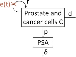
Schema of the secretion of PSA by prostate and cancer cells. PSA is expressed in ng.mL⁻¹ and C in mL⁻¹. r is the rate of prostatic cells proliferation in absence of treatment (day⁻¹), d the rate of prostatic cells elimination (day⁻¹), p the rate of PSA secretion by C (ng.day⁻¹), δ the rate of PSA elimination (day⁻¹), and e(t) the time-dependent treatment effect

Treatment is initiated at t = 0; PSA(0) = PSA₀ and C(0) = C₀ are PSA value and the number of prostatic cells at treatment initiation, respectively. Here, treatment is assumed to be constantly effective until a certain time, T_esc, after what tumor escapes and treatment has no longer an effect:

$$e\left(t\right)=\left\{\begin{array}{l}\epsilon \mathit{if}t\le T_{\mathrm{e}\mathrm{s}\mathrm{c}}\hfill \\ 0\mathit{if}t>T_{\mathrm{e}\mathrm{s}\mathrm{c}}\hfill \end{array}\right.$$ 2

Further, we made the assumption of quasi steady-state at treatment initiation, and thus, $C_0=\frac{\delta \times {\mathrm{P}\mathrm{S}\mathrm{A}}_0}{p}$. With this piecewise constant treatment effect (Eq. 2), the model (Eq. 1) has an analytical solution given by:

$$\begin{array}{ll}\text{PSA}\left(t,\psi \right)=\hfill & \left\{\begin{array}{ll}\frac{\delta {\mathrm{P}\mathrm{S}\mathrm{A}}_0}{r\left(1-\epsilon \right)-d+\delta }{e}^{\left(r\left(1-\epsilon \right)-d\right)t}+\left[{\mathrm{P}\mathrm{S}\mathrm{A}}_0-\frac{\delta {\mathrm{P}\mathrm{S}\mathrm{A}}_0}{r\left(1-\epsilon \right)-d+\delta }\right]e^{-\delta t}\hfill & \mathit{if}t\le T_{\mathrm{e}\mathrm{s}\mathrm{c}}\hfill \\ \frac{\delta {\mathrm{P}\mathrm{S}\mathrm{A}}_0}{r-d+\delta }{e}^{\left(r-d\right)t-r\epsilon T_{\mathrm{e}\mathrm{s}\mathrm{c}}}+\left[\mathrm{P}\mathrm{S}\mathrm{A}\left(T_{\mathrm{e}\mathrm{s}\mathrm{c}}\right)-\frac{\delta {\mathrm{P}\mathrm{S}\mathrm{A}}_0{e}^{\left(r\left(1-\epsilon \right)-d\right)T_{\mathrm{e}\mathrm{s}\mathrm{c}}}}{r-d+\delta }\right]e^{-\delta \left(t-T_{\mathrm{e}\mathrm{s}\mathrm{c}}\right)}\hfill & \mathit{if}t>T_{\mathrm{e}\mathrm{s}\mathrm{c}}\hfill \end{array}\right.\hfill \end{array}$$ 3

Because only four parameters can be identified from Eq. 3, we fixed d to 0.046 day⁻¹, corresponding to a half-life of tumor cells of 15 days, consistent with an apoptotic index of 5% in metastatic prostate cancer (21). Moreover, we fixed δ to 0.23 day⁻¹, corresponding to a PSA half-life in blood of about 3 days (22). Thus, PSA kinetics was defined by the vector parameter ψ = {r, PSA₀, ε, T_esc}.

Statistical Model for PSA Measurements

Let y_ij denote the jth longitudinal measurement of log(PSA + 1) for the individual i at time t_ij, where i = 1, …, N, j = 1, …, n_i, N is the number of subjects, and n_i the number of measurements in subject i. The nonlinear mixed-effect model (NLMEM) for PSA is defined as follows:

$$y_{ij}=\log (\mathrm{P}\mathrm{S}\mathrm{A}(t_{ij},{\psi }_i)+1)+\sigma e_{ij}$$ 4

where PSA is given by the formula (Eq. 3), ψ_i is the vector of the individual parameters, and e_ij is the residual error which follows a standard normal distribution with mean 0 and variance 1. The vector of the individual parameters ψ_i is decomposed as fixed effects μ = {r, PSA₀, ε, T_esc} representing median effects of the population and random effects η_i specific for each individual. It is assumed that η_i ∼ N(0, Ω) with Ω the variance-covariance matrix. In this work, Ω is supposed to be diagonal. Each diagonal element ω_q² represents the variance of the qth component of the random effect vector η_i. We assumed log-normal distribution for r, PSA₀, and T_esc:

$$\log \left({\psi }_{q,i}\right)=\log \left({\mu }_q\right)+{\eta }_{q,i}$$

and logit-normal distribution for ε:

$\mathrm{logit}\left({\epsilon }_i\right)=\mathrm{logit}\left({\mu }_{\epsilon }\right)+{\eta }_{e,i}\mathrm{with}\mathrm{logit}\left(x\right)=log\left(\frac{x}{1-x}\right)$ for 0 < x < 1.

The population parameter vector of PSA noted θ_l is composed of {μ, Ω, σ}.

Statistical Model for Survival

Let X_i denote the time to event and C_i the censoring time for the ith subject. Survival data (T_i, δ_i) are observed in all individuals, where T_i = min(X_i, C_i) and δ_i = 1, if X_i ≤ C_i, 0 otherwise. For the event process, we used a hazard function of the form:

$$h_i\left(t\left|\mathrm{P}\mathrm{S}\mathrm{A}\left(t,{\psi }_i\right)\right.\right)=h_0\left(t\right)exp\left(\beta \mathrm{P}\mathrm{S}\mathrm{A}\left(t,{\psi }_i\right)\right)$$ 5

where the baseline hazard function, h₀, is a Weibull hazard function $h_0\left(t\right)=\frac{k}{\lambda }{\left(\frac{t}{\lambda }\right)}^{k-1}$. The parameter β measures the strength of the association between the PSA kinetics and the risk of death. If β = 0, the survival process is independent on the PSA evolution, and survival data can be fitted by a Weibull model without adjusting for PSA. If β ≠ 0, the survival process depends on the PSA kinetics. The survival parameters to estimate are θ_s = {λ, k, β}.

Joint Model

Joint models assume conditional independence: given the random effects η_i, longitudinal measurements and survival events are independent. All parameters θ = {θ_l, θ_s} are simultaneously estimated. Thus, the joint log-likelihood for the subject i can be written as follows (23):

$$l_i\left(\theta \right)=log{\displaystyle \int p\left(y_i\left|{\eta }_i;\theta \right.\right)}\left\{h_i{\left(T_i\left|{\eta }_i\right.\theta \right)}^{{\delta }_i}{S}_i\left(T_i\left|{\eta }_i\right.\theta \right)\right\}p\left({\eta }_i;\theta \right)d{\eta }_i$$ 6

where S_i(t|η_i;θ) = exp (−∫^t₀h₀(s|η_i;θ) exp (βPSA (s, ψ_i))ds) is the survival function conditionally on the random effects, p(y_i|η_i;θ) the density of the longitudinal observations conditionally on the random effects, and p(η_i; θ) the density of the random effects.

Two-Stage Model

In order to simplify the heavy calculations involved by Eq. 6, one may also use a two-stage approach. In the first step, PSA kinetics parameters (θ_l) are estimated assuming complete independence of PSA kinetics and survival and the Empirical Bayes Estimates (EBEs), defined as the mode of the conditional distribution $p\left({\psi }_i\left|y_i\right.{\widehat{\theta }}_l\right)$, are used to provide individual parameters, noted ${\widehat{\psi }}_i$. In the second step, the survival parameters (θ_s) are estimated maximizing the usual log-likelihood $l\left({\theta }_s\right)={\displaystyle {\sum }_{i=1}^{n}log}\left\{h_i{\left(T_i\left|\mathrm{P}\mathrm{S}\mathrm{A}\left(t,{\widehat{\psi }}_i\right);{\theta }_s\right.\right)}^{{\delta }_i}{S}_i\left(T_i\left|\mathrm{P}\mathrm{S}\mathrm{A}\left(t,{\widehat{\psi }}_i\right);{\theta }_s\right.\right)\right\}$.

This method is analogous to the sequential method called “Individual Pharmacokinetic Parameters” (IPP) used in pharmacometric field to handle pharmacokinetic/pharmacodynamic (PKPD) data (14).

Joint Sequential Model

In order to reduce the number of parameters to estimate in Eq. 6, an alternative consists of first estimating population PSA kinetic parameters, as done in the two-stage model, and then estimating parameters related to survival (θ_s) fixing the all population PSA parameters (θ_l) in Eq. 6 to the values obtained at the previous stage. This method, inspired from the “Population PK parameter and individual PK data” for the combined analysis of PKPD data, has been shown to limit the bias compared to two-stage approach (14).

SIMULATION STUDY

Design

Simulation setting was inspired by one arm of a phase III study of clinical development of chemotherapy for metastatic prostate cancer (3). M = 100 datasets with N = 500 patients were simulated with PSA measurements every 3 weeks for 2 years (i.e., the last possible measurement time was at t = 735 days), leading to a maximum of 36 observations per patient (Table I). Follow-up was censored at t = 735, and no other mechanism than death was considered for dropout. For the simulation of the time to death, k was fixed to 1.5, and three values for β were considered: 0, 0.005, and 0.02, corresponding to “no link”, “low link” and “high link” between PSA kinetics and survival, respectively. In order to maintain a comparable amount of PSA measurements across scenarios, λ was determined in each scenario such that the probability of survival at the end of the follow-up (i.e., 735 days) was equal to 25% with the median PSA kinetic parameters (Table I), leading to λ = 580, 765, and 2150 in scenarios “No link”, “Low link” and “High link”, respectively (Table II). Lastly, we evaluated the effects of having both a large baseline risk and a strong effect of PSA kinetics by setting β = 0.02 and λ = 580 in the scenario called “Short survival”. Figure 2 shows the survival functions for these four scenarios for the “median patient”, i.e., a virtual patient having PSA kinetic parameters equal to the median values in the population.

Table I.

Values of the Population PSA Parameters Used for the Simulations in all Scenarios

	Fixed effects	Transformation	Inter-individual standard deviation (ω)
r (day−1)	0.05	log-normal	0.1
PSA0(ng.mL−1)	80	log-normal	0.6
ε	0.3	logit-normal	1.5
Tesc (day)	140	log-normal	0.6
σ	0.36	-	-

Table II.

Values of the Population Survival Parameters Used for the Simulations of the Four Scenarios

	Scenario No link	Scenario Low link	Scenario High link	Scenario Short survival
β	0	0.005	0.02	0.02
λ (day)	580	765	2150	580
k	1.5	1.5	1.5	1.5

Fig. 2.

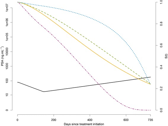
Typical evolution of PSA(t) (solid black) and survival functions in the typical patient (who have the fixed effects of the Table I as PSA parameters) for the scenarios “No link” (β = 0, λ = 580) (solid orange), “Low link” (β = 0.005, λ = 765) (dashed green), “High link” (β = 0.02, λ = 2150) (dotted blue), and “Short survival” (β = 0.02, λ = 580) (dotdash purple)

In order to take into account the effect of withdrawals from PSA follow-up, we also explored additional scenarios where PSA and/or vital status were censored in case of PSA progression defined as an increase of 25% above the nadir and of at least 2 ng.mL compared to nadir (see Supplementary File 1).

All simulations were carried out with the R software version 3.0.1 (24).

Parameter Estimation

The estimation of two-stage, joint sequential, and joint models was performed for each dataset and each scenario using the Stochastic Approximation Expectation-Maximization (SAEM) algorithm in the software Monolix version 4.2.2.

The initial values of the parameters were those used for the scenario “No link.” Minus twice log-likelihood (−2LL) was calculated by Importance Sampling, fixing the Monte-Carlo sizes to achieve a sufficient level of precision for Likelihood Ratio Test (LRT) to 100,000 Monte-Carlo sizes for the scenario “No link,” 20,000 for the other scenarios in joint and joint sequential models, and 2,000 in two-stage model.

SAEM was run using one chain, and we verified that using three chains, as suggested in a related context (19), gave similar results. Central Processing Unit (CPU) times for parameter estimations and −2LL estimations were recorded on a i7 64 bits 3.33 GHz.

Evaluation Criteria

We used Relative Estimation Errors defined by: $\mathrm{R}\mathrm{E}\mathrm{E}\left({\widehat{\theta }}_m\right)=\frac{{\widehat{\theta }}_m-{\theta }^{\ast }}{{\theta }^{\ast }}\times 100$, where θ^∗ and ${\widehat{\theta }}_m$ are the true and estimated parameters, respectively, for dataset m, m = 1…M. Boxplots of the REEs with the 10 and 90% percentiles were plotted. When β = 0 (scenario “No link”), the boxplot of the absolute estimation error, ${\widehat{\beta }}_k$, with the 10 and 90% percentiles was plotted.

The type 1 error and power were calculated as the proportion among the M datasets for which LRT (called in the following “uncorrected LRT”) led to reject the null hypothesis H₀: β = 0. The type 1 error was evaluated in the scenario “No link,” and the power was calculated for the three other scenarios. The significance level of the tests α for the observed type 1 error was fixed to 0.05, leading to a 95% prediction interval for 100 replicates equal to [0.7–9.3%].

In some cases, the estimation of −2LL, which relies on a stochastic approximation, was associated with a non-negligible standard error. Because this can lead to an inflation of the type 1 error, we also evaluated a “corrected LRT.” In this test, H₀ was rejected if − 2LL (H₀) + 2LL (H₁) belonged to $({\chi }_1^2+z_{\alpha }\sqrt{s{e}_{-2\mathrm{L}\mathrm{L}}{\left(H_0\right)}^2+s{e}_{-2\mathrm{L}\mathrm{L}}{\left(H_1\right)}^2};\mathrm{\infty })$ where −se_−2LL(H₀) and se_−2LL(H₁) are the estimated standard errors of −2LL under H₀ and H₁, respectively, whereas χ²₁ and z_α are the chi-square value with one degree of freedom and the αth quantile of the standard normal distribution, respectively. $\sqrt{s{e}_{-2\mathrm{L}\mathrm{L}}{\left(H_0\right)}^2+s{e}_{-2\mathrm{L}\mathrm{L}}{\left(H_1\right)}^2}$ is the uncertainty for the sum of the two estimated −2LL. We used a corrected LRT if $z_a\sqrt{s{e}_{-2LL}{\left(H_0\right)}^2+s{e}_{-2\mathrm{L}\mathrm{L}}{\left(H_1\right)}^2}$ was non-negligible compared to χ²₁, i.e., for a significance level of 5%, se_− 2LL(H₀)² or se_− 2LL(H₁)² non-negligible compared to 2.

RESULTS

Simulated Data

Figure 3 shows the spaghetti plots along with the Kaplan-Meier curves of one typical dataset for each of the four scenarios. Because the scenario “No link” assumes that death does not depend on PSA kinetics, PSA rebound after loss of treatment efficacy (at time T_esc) was more frequently observed than in the three other scenarios. As expected (see Methods), the numbers of measurements in the first three scenarios were largely similar (Table III). In the last scenario where both the baseline hazard function and the effect of PSA kinetics were large, early events frequently occurred and the total amount of PSA data was much smaller.

Fig. 3.

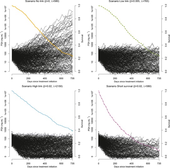
Spaghetti plots (black lines) and estimated Kaplan-Meier curves (colored lines) for one typical dataset (N = 500) for each of the four scenarios

Table III.

Number of PSA Measurements Per Patient and Median Survival in the Total Number of Simulated (50,000) Patients for the Four Simulated Scenarios

Number of PSA measurements	Scenario No link	Scenario Low link	Scenario High link	Scenario Short survival
1–5	7%	7%	8%	29%
6–10	12%	13%	10%	20%
11–20	26%	31%	22%	26%
21–35	30%	29%	21%	17%
36	24%	21%	39%	8%
Median survival (day)	457	414	552	217

Estimation Performance

No bias was observed in the scenario “No link” regardless of the approach. In the two-stage approach, increasing effect of PSA on survival led to higher levels of bias (Figs. 4 and 5). In particular, there was a systematical underestimation of the PSA effect on survival with median (Q1;Q3) REE for β which equals to −8.4% (−12.6; −4.1), −14.8% (−18.9; −10.2), and −9.1% (−16.7; −5.7) in scenarios “Low link”, “High link” and “Short survival,” respectively. The bias was corrected by using joint sequential models or joint models, with median (Q1;Q3) REE for β of 0.005% (−3.6; 5.3), −0.6% (−3.3; 2.9), and 0.03% (−4.8; 5.7) in scenarios “Low link”, “High link” and “Short survival,” respectively, for this latter method. Although the three approaches led to low REEs for the almost all parameters of PSA kinetics (Fig. 4), a bias was observed for the proliferation rate of tumor cells, r, with median (Q1;Q3) REE which equals to −0.4% (−0.7; −0.05), −0.8% (−1.0; −0.5), and −1.2% (−1.8; −0.7) in scenarios “Low link”, “High link” and “Short survival,” respectively, when using the two-stage or joint sequential approach. Here as well, the bias was largely reduced when using a joint model, with median (Q1;Q3) REE for r which equals to 0.01% (−0.4; 0.3), −0.004% (−0.3; 0.2), and −0.08% (−0.6; 0.5), in scenarios “Low link”, “High link” and “Short survival,” respectively. Of note, large REE was found for the parameters λ and k (|REE| > 30%) in the scenario “High link” when using joint and joint sequential models, due to the presence of a local extremum of the likelihood function.

Fig. 4.

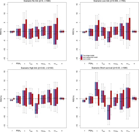
Boxplots of the relative estimation errors for parameters related to PSA for two-stage model (blue), joint sequential model (purple), and joint model (red), for the four scenarios. Top left: scenario No link (β = 0, λ = 580), top right: scenario Low link (β = 0.005, λ = 765), bottom left: scenario High link (β = 0.02, λ = 2150) and bottom right: scenario Short survival (β = 0.02, λ = 580)

Fig. 5.

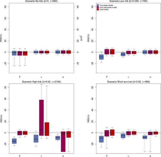
Boxplots of the relative estimation errors for parameters related to survival (in % except for β of the scenario No link for which estimated values are represented) for two-stage model (blue), joint sequential model (purple), and joint model (red), for the four scenarios. Top left: scenario No link (β = 0, λ = 580), top right: scenario Low link (β = 0.005, λ = 765), bottom left: scenario High link (β = 0.02, λ = 2150), and bottom right: scenario Short survival (β = 0.02, λ = 580)

Lastly, we also considered additional scenarios where PSA data and/or vital status was censored in case of PSA increase (see Supplementary File 1). Although the precision of the parameter estimates was deteriorated due to the reduction in the amount of data available, no substantial bias in the PSA kinetic parameters was found using joint model. However, bias was found in survival-related parameters, in particular when both PSA and vital status were censored after disease progression and this bias systematically led to an overestimation of the hazard function.

Test Performance

The uncorrected LRT led to a type 1 error of 21, 9, and 12% for the joint model, the joint sequential model, and the two-stage model, respectively, i.e., outside the 95% prediction interval ([0.7–9.3%] for 100 replicates). The use of a corrected LRT (see methods) led to a smaller type 1 error of 4, 3 and 12% for the joint model, the joint sequential model, and the two-stage model, respectively. The reason why the type 1 errors for the two-stage model with or without correction were similar is due to the fact that the standard error of −2LL was negligible with this model (<10⁻⁴). For the scenarios with β ≠ 0, the power was 100% with all three models, regardless of the correction.

Computation Time

Mean CPU times for the simultaneous estimation of the 12 parameters using joint model were about five times larger than the total CPU times using two-stage model (70 vs 14 min) and about 1.2 times larger than the total CPU times using joint sequential model (70 vs 59 min), ignoring the time for specific data manipulation required for setting the two-stage and joint sequential approaches. Mean CPU times for the −2LL estimation using joint model (respectively, joint sequential model) and 100,000 chains were about 3.1 (respectively, 3.6) times larger than when using the joint approach and 20,000 chains (264 vs 86 min (respectively, 207 vs 57 min)) but led to a mean se_−2LL(H₁) of 1.96 vs 5.14 (respectively, 2.40 vs 5.90).

DISCUSSION

Numerical complexities have long limited the use of joint models to longitudinal processes defined by linear mixed-effect models (7,10,15). Here, we evaluated by simulation, in the context of PSA and survival in metastatic prostate cancer, the capability of a new feature of the Stochastic Approximation Expectation-Maximization algorithm in Monolix to estimate the parameters of a joint model where the longitudinal process was defined by a nonlinear model. And we compared the results to two simplified approaches, two-stage and joint sequential models.

We found that joint model provided unbiased parameters of both longitudinal and survival processes. In contrast, the use of a two-stage model (5,25) led to large biases when PSA kinetics and survival were linked. In particular, the impact of the biomarker kinetics on the survival, as measured by the link parameter β, was systematically underestimated, consistent with results found in linear mixed-effect model (8,9). Beside survival parameters, a bias on the tumor proliferation rate, r, which is the driving force for the increase in PSA, was also observed in scenarios with β ≠ 0. The fact that no such bias occurred when using joint model shows that the simultaneous estimation of the hazard function also improved the estimation of the longitudinal parameters. Moreover, a two-stage approach led to an inflation of type 1 error (i.e., concluding to an effect of PSA on survival while there is none) which could be explained by the shrinkage of the EBEs in patients with short survival (26). By construction, the joint sequential model led to the same biases on PSA longitudinal parameters than the two-stage model, but the estimation of survival parameters was close to that obtained with the joint model. This, therefore, suggests that joint sequential model could be a relevant approach when joint model cannot be performed.

In spite of the increasing numerical capability, the likelihood of joint models remains particularly complex to calculate. Here, we reported that the likelihood was estimated with a relatively large uncertainty. Increasing the Monte-Carlo sizes led to smaller standard errors of the likelihood but considerably increased the computation time. The impact of this error on type 1 error was in part accounted by using a corrected likelihood ratio test (LRT). However, more studies will be needed to precisely determine when this correction is necessary and whether it can be improved. Here, for instance, the corrected rejection region did not take into account the covariance between the likelihood calculated under the null and alternative hypotheses. Although the Wald test may be an alternative, we found here that standard errors of the estimates tended to be smaller than the root mean-squared errors (RMSE), indicating a potential underestimation of the standard errors. Furthermore, and in spite of the stochastic algorithm, the estimation of parameters related to survival was complicated in some cases by the existence of local extremum of the likelihood function. This stresses the need, in practice, to perform several runs of likelihood maximization using different initial values.

The main advantage of nonlinear models is the possibility to develop physiological models based on nonlinear differential equations, which naturally integrate the correlations between the different biomarkers. In this study, we used a rather simple model where the treatment effectiveness was piecewise constant, which allowed us to derive a biexponential analytical solution for the PSA kinetics. However, this model may clearly be oversimplistic, and more complex models will be needed that rely on several markers, such as tumor size or drug pharmacokinetics. The facilitated use of these models via joint models holds the promise that the determinants of survival may be much better characterized (20).

Regarding the survival model, we restricted here to a rather simple fully parametric model, where the baseline hazard function was a Weibull model (27), and the hazard function was related to the current PSA values. In practice, complex survival models could be evaluated, and standard tools for model selection (e.g., AIC or BIC) could be used to evaluate the effect of various transformations of the biomarker, such as the derivative or the cumulative value of PSA. Lastly, with a fully parametric model, the prediction and the simulation of the individual hazard function can easily be performed, making possible to guide treatment adaptation in a dynamic manner (28).

CONCLUSION

SAEM algorithm implemented in Monolix was shown to provide precise estimates for joint models where the longitudinal model was defined by a nonlinear mixed-effect model. This opens the way for a more systematic use of joint models and a better understanding of the relationship between biomarker kinetics and survival, especially in the field of metastatic cancer where survival and nonlinear biomarker kinetics are intrinsically related.

References

- 1.Ferlay J, Soerjomataram I, Ervik M, Dikshit R, Eser S, Mathers C, et al. GLOBOCAN 2012 v1.0, Cancer Incidence and Mortality Worldwide: IARC CancerBase [Internet]. Lyon, France: International Agency for Research on Cancer. 2013. Report No.: 11. Available from: http://globocan.iarc.fr.
- 2.Howlader N, Noone A, Krapcho M, Garshell J, Miller D, Altekruse S, et al. SEER Cancer Statistics Review, 1975–2011 [Internet]. National Cancer Institute. 2013. Available from: http://seer.cancer.gov/csr/1975_2011/.
- 3.Tannock IF, Fizazi K, Ivanov S, Karlsson CT, Fléchon A, Skoneczna I, et al. Aflibercept versus placebo in combination with docetaxel and prednisone for treatment of men with metastatic castration-resistant prostate cancer (VENICE): a phase 3, double-blind randomised trial. Lancet Oncol. 2013;14:760–8. doi: 10.1016/S1470-2045(13)70184-0. [DOI] [PubMed] [Google Scholar]
- 4.Petrylak DP, Ankerst DP, Jiang CS, Tangen CM, Hussain MHA, Lara PN, et al. Evaluation of prostate-specific antigen declines for surrogacy in patients treated on SWOG 99–16. J Natl Cancer Inst. 2006;98:516–21. doi: 10.1093/jnci/djj129. [DOI] [PubMed] [Google Scholar]
- 5.Proust-Lima C, Taylor JMG, Williams SG, Ankerst DP, Liu N, Kestin LL, et al. Determinants of change in prostate-specific antigen over time and its association with recurrence after external beam radiation therapy for prostate cancer in five large cohorts. Int J Radiat Oncol Biol Phys. 2008;72:782–91. doi: 10.1016/j.ijrobp.2008.01.056. [DOI] [PMC free article] [PubMed] [Google Scholar]
- 6.Murawska M, Rizopoulos D, Lesaffre E. A two-stage joint model for nonlinear longitudinal response and a time-to-event with application in transplantation studies. J Probab Stat [Internet]. 2012 [cited 2014 Apr 23];2012. Available from: http://www.hindawi.com/journals/jps/2012/194194/abs/.
- 7.Wu L, Liu W, Yi GY, Huang Y. Analysis of longitudinal and survival data: joint modeling, inference methods, and issues. J Probab Stat [Internet]. 2011 [cited 2013 Jul 10];2012. Available from: http://www.hindawi.com/journals/jps/2012/640153/abs/.
- 8.Sweeting MJ, Thompson SG. Joint modelling of longitudinal and time-to-event data with application to predicting abdominal aortic aneurysm growth and rupture. Biom J. 2011;53:750–63. doi: 10.1002/bimj.201100052. [DOI] [PMC free article] [PubMed] [Google Scholar]
- 9.Ibrahim JG, Chu H, Chen LM. Basic concepts and methods for joint models of longitudinal and survival data. J Clin Oncol. 2010;28:2796–801. doi: 10.1200/JCO.2009.25.0654. [DOI] [PMC free article] [PubMed] [Google Scholar]
- 10.Taylor JM, Wang Y. Surrogate markers and joint models for longitudinal and survival data. Control Clin Trials. 2002;23:626–34. doi: 10.1016/S0197-2456(02)00234-9. [DOI] [PubMed] [Google Scholar]
- 11.Wulfsohn MS, Tsiatis AA. A joint model for survival and longitudinal data measured with error. Biometrics. 1997;53:330. doi: 10.2307/2533118. [DOI] [PubMed] [Google Scholar]
- 12.Tsiatis AA, Davidian M. Joint modeling of longitudinal and time-to-event data: an overview. Stat Sin. 2004;14:809–34. [Google Scholar]
- 13.Hsieh F, Tseng Y-K, Wang J-L. Joint modeling of survival and longitudinal data: likelihood approach revisited. Biometrics. 2006;62:1037–43. doi: 10.1111/j.1541-0420.2006.00570.x. [DOI] [PubMed] [Google Scholar]
- 14.Zhang L, Beal SL, Sheiner LB. Simultaneous vs. sequential analysis for population PK/PD data I: best-case performance. J Pharmacokinet Pharmacodyn. 2003;30:387–404. doi: 10.1023/B:JOPA.0000012998.04442.1f. [DOI] [PubMed] [Google Scholar]
- 15.Henderson R, Diggle P, Dobson A. Joint modelling of longitudinal measurements and event time data. Biostatistics. 2000;1:465–80. doi: 10.1093/biostatistics/1.4.465. [DOI] [PubMed] [Google Scholar]
- 16.Rizopoulos D. Joint models for longitudinal and time-to-event data: with applications in R. CRC Press. 2012. p. 275
- 17.Hu C, Sale ME. A joint model for nonlinear longitudinal data with informative dropout. J Pharmacokinet Pharmacodyn. 2003;30:83–103. doi: 10.1023/A:1023249510224. [DOI] [PubMed] [Google Scholar]
- 18.Björnsson MA, Friberg LE, Simonsson USH. Performance of nonlinear mixed effects models in the presence of informative dropout. AAPS J. 2014;17:245–55. doi: 10.1208/s12248-014-9700-x. [DOI] [PMC free article] [PubMed] [Google Scholar]
- 19.Vigan M, Stirnemann J, Mentré F. Evaluation of estimation methods and power of tests of discrete covariates in repeated time-to-event parametric models: application to Gaucher patients treated by imiglucerase. AAPS J. 2014;16:415–23. doi: 10.1208/s12248-014-9575-x. [DOI] [PMC free article] [PubMed] [Google Scholar]
- 20.Mbogning C, Bleakley K, Lavielle M. Joint modelling of longitudinal and repeated time-to-event data using nonlinear mixed-effects models and the stochastic approximation expectation–maximization algorithm. J Stat Comput Simul. 2015;85:1512–28.
- 21.Tu H, Jacobs SC, Borkowski A, Kyprianou N. Incidence of apoptosis and cell proliferation in prostate cancer: relationship with TGF-β1 and bcl-2 expression. Int J Cancer. 1996;69:357–63. doi: 10.1002/(SICI)1097-0215(19961021)69:5<357::AID-IJC1>3.0.CO;2-4. [DOI] [PubMed] [Google Scholar]
- 22.Polascik TJ, Oesterling JE, Partin AW. Prostate specific antigen: a decade of discovery—what we have learned and where we are going. J Urol. 1999;162:293–306. doi: 10.1016/S0022-5347(05)68543-6. [DOI] [PubMed] [Google Scholar]
- 23.Rizopoulos D, Verbeke G, Lesaffre E. Fully exponential Laplace approximations for the joint modelling of survival and longitudinal data. J R Stat Soc Ser B Stat Methodol. 2009;71:637–54. doi: 10.1111/j.1467-9868.2008.00704.x. [DOI] [Google Scholar]
- 24.R Development Core Team. R Development Core Team (2013). R: A language and environment for statistical computing. R Foundation for Statistical Computing, Vienna, Austria. ISBN 3-900051-07-0, URL http://www.R-project.org. R Foundation for statistical computing, Vienna, Austria.
- 25.Taylor JMG, Yu M, Sandler HM. Individualized predictions of disease progression following radiation therapy for prostate cancer. J Clin Oncol. 2005;23:816–25. doi: 10.1200/JCO.2005.12.156. [DOI] [PubMed] [Google Scholar]
- 26.Ribba B, Holford N, Mentré F. The use of model-based tumor-size metrics to predict survival. Clin Pharmacol Ther. 2014;96:133–5. doi: 10.1038/clpt.2014.111. [DOI] [PubMed] [Google Scholar]
- 27.Yu M, Law NJ, Taylor JMG, Sandler HM. Joint longitudinal survival cure models and their application to prostate cancer. Stat Sin. 2004;14:835–62. [Google Scholar]
- 28.Ribba B, Holford NH, Magni P, Trocóniz I, Gueorguieva I, Girard P, et al. A review of mixed-effects models of tumor growth and effects of anticancer drug treatment used in population analysis. CPT Pharmacomet Syst Pharmacol. 2014;3:e113. doi: 10.1038/psp.2014.12. [DOI] [PMC free article] [PubMed] [Google Scholar]
Associated Data
This section collects any data citations, data availability statements, or supplementary materials included in this article.
Supplementary Materials