RATIONALE AND APPLICATIONS OF SURVIVAL TREE AND SURVIVAL ENSEMBLE METHODS

Abstract

Classification and Regression Trees (CART), and their successors—bagging and random forests, are statistical learning tools that are receiving increasing attention. However, due to characteristics of censored data collection, standard CART algorithms are not immediately transferable to the context of survival analysis. Questions about the occurrence and timing of events arise throughout psychological and behavioral sciences, especially in longitudinal studies. The prediction power and other key features of tree-based methods are promising in studies where an event occurrence is the outcome of interest. This article reviews existing tree algorithms designed specifically for censored responses as well as recently developed survival ensemble methods, and introduces available computer software. Through simulations and a practical example, merits and limitations of these methods are discussed. Suggestions are provided for practical use.

1. Introduction

Survival analysis is a branch of statistical methods for investigating event occurrence— whether events occur and when events occur. Survival tree and survival ensemble methods are statistical learning techniques adapted to right-censored survival data. The counterparts of these techniques for more general categorical and continuous outcomes—Classification and Regression Trees (CART; Breiman, Friedman, Olshen, & Stone, 1984), bagging (Breiman, 1996) and random forests (Breiman, 2001), are better known and have promising merits (Strobl, Malley, & Tutz, 2009). There is a strong motivation for the adaptation of these methods to the survival contexts, because questions about the occurrence and timing of events arise throughout psychological and behavioral sciences (see Singer & Willett, 1991, 2003), especially in longitudinal studies. For example, researchers investigating the course of alcohol abuse are interested in the onset of the disorder (DeWit, Adlaf, Offord, & Ogborne, 2000) as well as post-treatment relapse (Mertens, Kline-Simon, Delucchi, Moore, & Weisner, 2012). Industrial and organizational psychologists study the rate and timing of employee turnover (e.g., Morita, Lee, & Mowday, 1993). Developmental psychologists ask the attainment of developmental milestones, for instance, the age of the acquisition of gender labeling (Zosuls et al., 2009).

The basis of tree methods lies in the recursive binary partitioning of a predefined covariate space into smaller and smaller regions, containing observations of homogeneous response (i.e., dependent variable) values. The resulting regions are called “nodes,” and each set in the final partition is called a “terminal node” or a “leaf.” The basic idea of recursive partitioning was first introduced by Morgan and Sonquist (1963) in their seminal work on Automatic Interaction Detection (AID), as reported by McArdle (2011). As a methodology it was formalized and generalized in CART by Breiman et al. (1984).

Any tree algorithm must include two key technical features: (a) the node splitting rule for generating the partition of the covariate space; and (b) the stopping rule, or the tree “pruning” criterion for deciding a tree’s optimal size. The unique problem with survival data, with necessarily censored responses, is that they typically do not have any natural measure of within node homogeneity or “impurity,” and this causes difficulty in inheriting the “impurity reduction” splitting rule directly from CART. For the same reason, a uniform “loss function” which assesses the cost brought about by the predicted value’s deviation from the true value, cannot be easily defined. So the cost-complexity of a tree, the key element in tree pruning (Breiman et al., 1984), cannot be evaluated. Although there has been discussion on the evaluation of the fit quality of a survival model in terms of prediction accuracy or explained variance (see a review by Schemper & Stare, 1996), which provide possible loss functions for censored outcomes, no measure has been widely accepted.

In this paper we introduce available survival tree algorithms and some recently developed survival ensemble methods which aggregate a large number of survival trees. We first explain the rationale of these methods via a practical example. Second, we review existing survival tree algorithms and compare their performance via simulations. Third, we introduce several recent adaptations of bagging and random forests to the survivor data, and evaluate the performance of these methods via simulations. Finally, we offer a general discussion of these methods and provide suggestions for their practice use.

2. A Practical Example

We explain the rationale of survival tree and survival ensemble methods through a simple example. The data are illustrated in Singer and Willett’s book (2003), and are shared on the website of the book (http://www.ats.ucla.edu/stat/examples/alda/). These data were originally collected by Henning and Frueh (1996) who tracked the criminal history of 194 inmates released from a medium security prison. The event of interest is whether the former inmates were re-arrested, and if so, how soon since their release (in months). During the period of data collection ranging between 1 day and 3 years, 106 (54.6 %) former inmates experienced the event. Three potential predictors are examined: (a) PERSONAL, a dichotomous variable indicating whether the former inmate had a history of person-related crimes (such as assault or kidnapping); (b) PROPERTY, a dichotomous variable indicating whether the former inmate was previously convicted for a property-related offense; and (c) AGE, the former inmate’s age at the time of release.

We begin this analysis by plotting Kaplan–Meier (KM) survival curves stratified by each of the three covariates in Figure 1. The age groups are formed by evenly splitting the age-sorted sample into four groups. This survival dataset has been studied deliberately by Singer and Willett (2003, see Chapter 14) using the Cox proportional hazards model (Cox, 1972; Cox & Oakes, 1984), and the results showed that all the three covariates are significant predictors of recidivism (see Table 1). Those inmates with a previous person-related crime were at a greater risk of re-incarceration. Similarly, the inmates with a previous property-related crime were also at a higher risk of re-incarceration. Also, as seen here, younger inmates at the time of last release seemed to be more likely to be re-arrested. More complex interactions were not examined.

Figure 1.

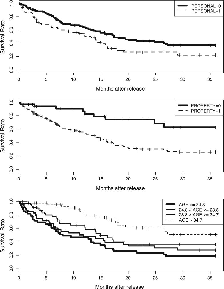
Kaplan–Meier survival curves by each covariate in the recidivism example.

Table 1.

Comparison of Cox regression, survival tree, bagging, and random survival forests in analyzing the recidivism data.

	Cox regression		Survival tree (conditional inference)		Baggin OOB Brier’s score	Random survival forests Variable importance
	Parameter estimate (SE)	Hazard ratio (SE)	Split	Groups
PERSONAL	.5691 (.2052)	1.7659(3642)	No	(1) AGE≤31.5;	.2142	.0222
PROPERTY	.9358 (.3509)	2.5482 (.8941)	Yes	(2) AGE>31 and PROPERTY =1;	.2142 .2178	.0222 .0117
	.9358 (.3509)	2.5482 (.8941)	Yes	(3) AGE>31 and PROPERTY = 0;	.2178	.0117
AGE	−.0667 (.0168)	.9355 (.0157)	Yes		.1991	.0341

OOB Brier’s scores shown in the table are prediction errors of the bagging procedure without the covariate. The OOB Brier’s score with all covariates is .2123.

2.1. Survival Tree Analysis of the Recidivism Data

Next we use a survival tree method to analyze the same data. Here we use the algorithm developed by Hothorn, Hornik, and Zeileis (2006b) within a conditional inference framework. As the tree plot in Figure 2a shows, from the entire sample of 194 former inmates, the first split is on AGE at 31.5 years, separating a group of 123 inmates (denoted by Node 2) who were younger than 31.5 years at the time of release from the rest who were older than this age at the time of release (Node 3). A second split is made for Node 3 based on the value of PROPERTY, which means for those older than 31.5 years at the time of release, 51 of them with a previous property-related crime (Node 5) are separated from the remaining 20 inmates without (Node 4). So the final partition of the original sample results in three groups (see Table 1), each indicated by a Kaplan–Meier estimate in their respective terminal node.

Figure 2.

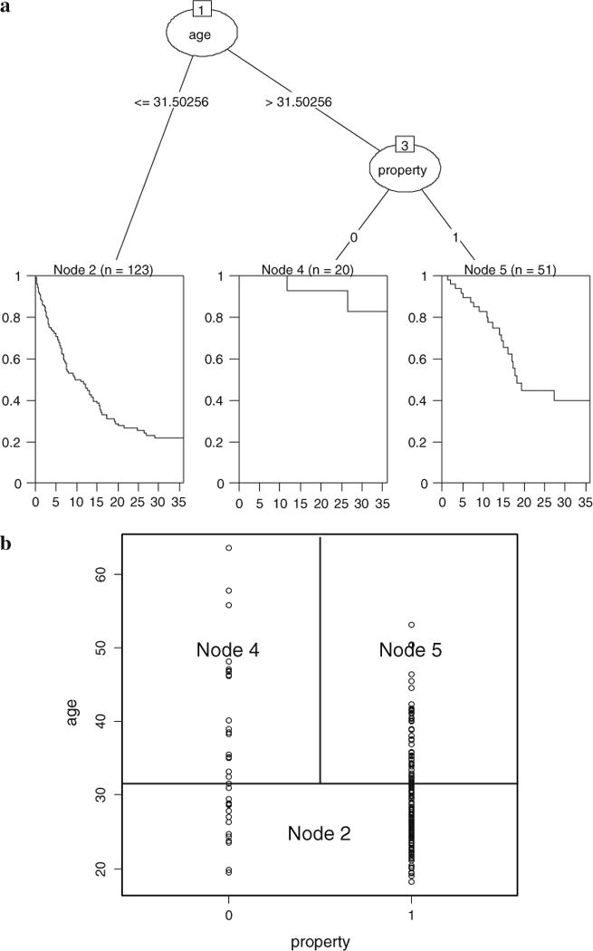
Partition of the recidivism data by means of a conditional inference survival tree. a (top): tree plot; b rectangular partition of the covariate space.

There are many common features that survival trees share with the general CART, as described in Berk (2008) and Strobl et al. (2009). First, at each step of the tree-growing procedure, the task is to find the single best split—the best predictor to split on and the best cut point of this predictor value—which increases the homogeneity of the observations (with regard to the response variable) within the resultant nodes. This can be observed from the shape of the Kaplan–Meier curves. The group in Node 2 who were younger at the time of last release, had a higher risk of recidivism, or, were likely to be re-incarcerated sooner. Most of them (approximately 80 %) did not survive the observation period of the study. Those persons who ended up in Node 4 were found to be at a lower risk, and most of them survived the observation period (approximately only 20 % rearrested). In this respect trees have a similar goal to that of discriminant analysis or latent class analysis—to identify homogenous subgroups of the original sample.

Secondly, trees are different from other methods in the way they carry out the sub-grouping. In most cases, the algorithms are used to divide the covariate space in the form of a “rectangular partition” (Strobl et al., 2009). As seen in Figure2b, in the condition of two predictors. In the example the inmates are grouped based on the value of AGE and the category in PROPERTY. In this approach, a split based on a linear combination of the predictors is not allowed.

Thirdly, the structure of the tree can imply interactions among the predictors. After the first split on AGE, the left Node 2 is not split further, while the right Node 3 is split again on PROPERTY. This indicates an interaction between AGE and PROPERTY—the effect of PROPERTY depends on the former inmate’s age at last release. For these below 31.5 years, their risk was high no matter they had a history of property-related crime or not, but for those older than 31.5 years, the absence of a previous property-related crime predicted a lower risk.

Lastly, the covariate PERSONAL does not show up in the tree, meaning that it is not selected to be a predictor. In tree methods, not all the covariates entering the program will be in the final model. Only the covariates that are the best split at one of the steps in computation, and at the same time, meet particular criteria to improve the overall performance of the tree (for the conditional inference trees, it is the p value), are selected. Note that in the Cox regression, the effect of PERSONAL, although weaker than that of PROPERTY, is also statistically significant.

2.2. Bagging Applied to the Recidivism Data

Next we apply a “bagging” procedure to the recidivism data. The term “Bagging” was used by Breiman (1996) as a shorter term for “bootstrap aggregation”—a procedure that aggregates over a number of (unpruned) single trees, each from a bootstrap sample of the data. The algorithm was originally invented by Breiman (1996) to overcome the instability and overfitting problems of single trees. In the procedure, observations that are not included in the bootstrap sample (called “out-of-bag” observations, OOB) can be used to calculate a more honest measure of prediction error.

The bagging algorithm used here was designed for survival outcomes by Hothorn, Lausen, Benner, and Radespiel-Tröger (2004). Prediction error is indexed by the integrated Brier score (Graf, Schmoor, Sauerbrei, & Schumacher, 1999), which measures the average discrepancy between the observed outcome and the estimated survival probability. We began by using all three covariates in the bagging procedure, and then excluded one of the covariates each time. One hundred bootstrap samples were drawn. The OOB Brier score was .2123 with all three covariates, .2142 when the covariate PERSONAL was excluded, .2178 when the covariate PROPERTY was excluded, and .1991 when the covariate AGE was excluded (see Table 1). There was slight increase in prediction error when PERSONAL or PROPERTY was removed. Surprisingly, removing the predictor AGE decreased the predictor error.

2.3. Random Survival Forests Applied to the Recidivism Data

Now we apply random survival forests to the recidivism data. We use the procedure developed by Ishwaran, Kogalur, Blackstone, and Lauer (2008), which was directly adapted from the original prescription laid out for random forests by Breiman (2003a, 2003b). Random forests add one additional step to the bagging procedure—in the construction of each tree, a pre-specified smaller number of predictors are randomly selected before each node is split, and the splitting variable is searched within the reduced set of predictors. The algorithm by Ishwaran et al. (2008) uses Harrell’s concordance index (C-index; Harrell, Califf, Pryor, Lee, & Rosati, 1982) as a measure of prediction error for survival data. This statistic is an estimate of the probability that, in a randomly selected pair of cases, the sequence of events that occur is successfully predicted (so prediction error is 1-C).

In the application, one thousand bootstrap samples were generated. The splitting rule used in calculating (or “growing”) survival trees was based on the log-rank statistic (Mantel, 1966; Peto & Peto, 1972), a test statistic for comparing the survival curves of two samples. The number of predictors randomly selected for each split was set to be two. The procedure obtained an OOB error rate of 37.48 %, better than a random guess of 50 %, suggesting that the three covariates are predictive of recidivism. In Figure 3, the left plot shows that the error rate was stabilized at around 400 trees. The right plot ranks the variable importance measure of the three covariates from high to low (their values are shown in Table 1). It shows that AGE is the strongest predictor, and PERSONAL seems to be more important than PROPERTY.

Figure 3.

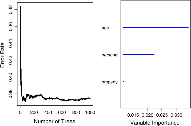
Survival forest error rate stabilization (left) and variable importance plot (right).

2.4. Comparison of the Results

The focus taken to approach the problem is quite different among the four illustrated methods. Cox regression examines each covariate’s effect based on hypothesis testing, survival tree focuses on classification, and bagging and random survival forests focus on prediction. The results from survival tree and survival ensemble methods seem to complement the results from traditional survival analysis (i.e., the Cox regression). However, at some point they disagree with each other; bagging suggests that AGE is not predictive of recidivism, and survival tree shows that there seems to be an interaction between AGE and PROPERTY. So the question arises—how trustworthy are survival tree and survival ensemble methods?

The answer to the question first depends on the performance of these algorithms. Take survival trees for example, Figure 4 is the tree result from a different survival tree algorithm with the splitting rule developed by LeBlanc and Crowley (1992). The stopping rule is that at least 60 observations must exist in a node in order for a split to be attempted, and at least 20 observations must exist in any terminal node. The first split is still on AGE at 31.5, but further splits are different from the previous tree in Figure 2, and this results in a different classification of the sample. In the next section we have a review of existing survival tree algorithms. We will revisit the recidivism example in later sections.

Figure 4.

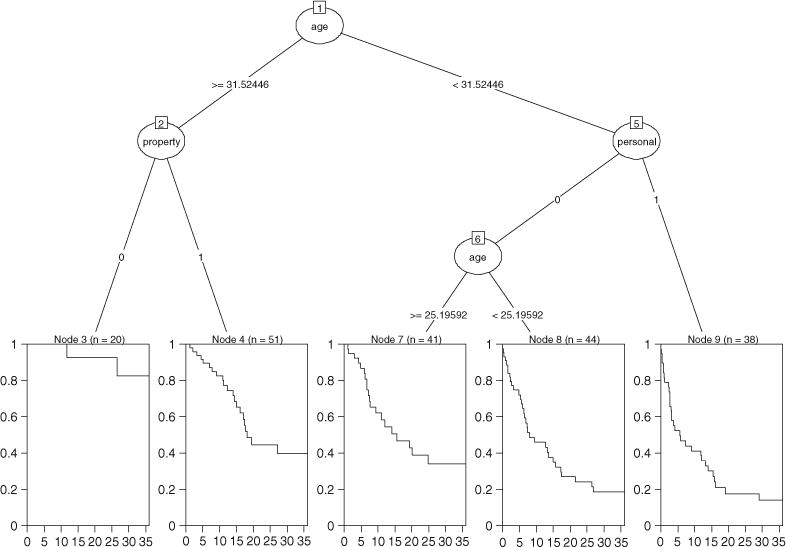
Tree plot for the recidivism data with a different survival tree algorithm.

3. A Brief Review of Survival Tree Algorithms

The first attempt to adapt the CART algorithm in the context of censored data seems to have been reported by Gordon and Olshen (1985). Since then, more than ten survival tree algorithms have been proposed, although only a few have been implemented in publicly available software. We summarize the main characteristics of these algorithms in Table 2.

Table 2.

Summary of published survival tree algorithms.

Author(s)	Splitting rule	Pruning rule	Implementation
Gordon and Olshen (1985)	Impurity (specifically defined based on KM curves) reduction	Cost-complexity pruning and cross-validation	STREE
Ciampi, Thiffault, Nakache, and Asselain (1986)	Log-rank test statistic	Akaike information criterion (AIC)	Splitting criterion implemented in STREE
Segal (1988)	Log-rank test statistic	Not available	Splitting criterion implemented in STREE
Butler, Gilpin, Gordon, and Olshen (1989) Davis and Anderson (1989)	Log-rank test statistic Exponential log-likelihood	A within-node measure Cost-complexity pruning
Therneau, Grambsch, and Fleming (1990)	Martingale residuals	Cost-complexity pruning and cross-validation
LeBlanc and Crowley (1992)	First step of full likelihood	Cost-complexity pruning and cross-validation	Splitting criterion implemented in R package “rpart;” STREE also has a slightly modified version.
LeBlanc and Crowley (1993)	Log-rank test statistic	Resampling and permutation
Intrator and Kooperberg (1995)	Log-rank test statistic	Cost-complexity pruning
Zhang and Singer (1999)	A weighted combination of impurity of the death indicator and impurity of the time	Cost-complexity pruning
Breiman (2002)	Probability .75 to split on time, and Probability .25 to split on a covariate	N/A (embedded within the survival forest algorithm)	Breiman (2003a, 2003b)
Molinaro, Dudoit, and van der Laan (2004)	An inverse probability of censoring weighted (IPCW) loss function	Cost-complexity pruning and cross-validation	Use R package “rpart” by providing IPCW weights
Hothorn et al. (2006b)	Minimum p value	Stop when no p value is below a pre-specified a-level	R package “party”

Molinaro et al. (2004) pointed out that survival tree algorithms can be placed into two categories based on their use of within-node homogeneity or between-node heterogeneity measures. The algorithms in the first category have inherited the fundamental basis of CART, in the sense that they rely on splitting rules which optimize a loss-based within-node homogeneity criterion, and use cost-complexity pruning and cross-validation to select an optimal-sized tree among a sequence of candidate trees. They differ in their definitions of the loss function. Gordon and Olshen (1985) created a measure of node impurity in the context of censored data by defining three possible shapes of survival curves (based on Kaplan–Meier calculations) which were regarded as “pure,” and the node impurity was then the deviation of the within-node survival curve from any of the three pure curves. Davis and Anderson (1989) based their split function on the negative log-likelihood, while assuming an exponential model for the baseline hazard function. Therneau et al. (1990) suggested using martingale residuals and this allows direct application of CART to survival outcomes. LeBlanc and Crowley (1992) used the first step of a full likelihood estimation procedure, assuming a proportional hazards model. Zhang (described in Zhang and Singer 1999) proposed a more straightforward approach by defining node impurity as a weighted combination of impurity of the binary death indicator (i.e., a dummy variable for whether or not a death has occurred) and the impurity of the time duration. Molinaro et al. (2004) argued that existing survival tree methods all chose the splitting and pruning criteria based on convenience of handling censored data, and did not reduce to the preferred choice for uncensored data. To address this problem, they proposed a unified methodology by defining an inverse probability of censoring weighted (IPCW) loss function.

In the second category of survival tree algorithms, the two sample log-rank test statistic is dominantly employed as the between-node heterogeneity measure. This approach, based on an alternative idea for splitting and pruning, is considered to deviate markedly from standard tree methodology (Molinaro et al., 2004). Ciampi et al. (1986) and Segal (1988) were the earliest to take this approach. However, Segal’s algorithm did not provide a solution for choosing the size of a tree. Intrator and Kooperberg (1995) modified Segal’s (1988) algorithm by adding a cost-complexity pruning. The algorithm by Ciampi et al. (1986) used the Akaike Information Criterion (AIC) for selecting the tree size, which is strongly related to the log-likelihood by adding a penalty based on the number of parameters. This method assumes asymptotic equivalence of AIC and cross-validation according to Stone (1974). LeBlanc and Crowley (1993) criticized that such an equivalence was not likely to hold in this particular setting. Instead, they used a pruning algorithm with optimal properties analogous to the CART pruning procedure, and used resampling and permutation techniques to select the tree size. Butler et al. (1989) also used the log-rank test statistic for splitting, but they used a within-node measure for pruning and selecting tree size.

More recently, Hothorn et al. (2006b) proposed a “conditional inference permutation test” for recursive partitioning. Based on a theory of permutation tests, it uses p value both as the splitting criterion (i.e., require a split with minimum p value) and as the stopping criterion (i.e., stop when no p value is below a pre-specified α-level) and therefore does not rely on a pruning procedure to select the tree size. They showed that this algorithm overcomes the selection bias towards predictors with many possible splits or missing values, a fundamental problem in the CART methods. For the special case of censored responses, they suggest choosing log-rank or Savage scores in the calculation and then proceed as for univariate continuous regression.

3.1. Available Computer Software

Although a number of survival tree algorithms have been proposed, only a few have been implemented and made available and (most importantly) convenient for practical researchers to use. Two R add-on packages—“rpart” (Therneau & Atkinson, 2010) and “party” (Hothorn, Hornik, Strobl, & Zeileis, 2010) provide implementation for survival trees. In particular, “rpart” uses the splitting rule by LeBlanc and Crowley (1992), and users can choose values of the two parameters “minsplit” and “minbucket” for a desirable tree size. “minspit” indicates the minimum number of observations in a node for a split to be attempted, and “minbucket” indicates the minimum number of observations in any terminal node. “Party” implements the conditional inference procedure by Hothorn et al. (2006b). Users can choose a parameter value for “mincriterion” (which is 1 − α) to select tree sizes, but the other two parameters “minsplit” and “minbucket” are available as well. Hothorn and Zeileis (2012) later provided a toolkit “partykit” that can convert a tree fitted using “rpart” to a tree that shares the same functionality as a tree fitted using “party” so that tree structures can be visualized in a standardized way. In our illustrations, trees fitted in “rpart” were all converted and plotted as “party” trees.

In addition to these, Zhang provides a free program STREE on his website based on the methods discussed in Chapter 8 of Zhang and Singer (1999). It implements five optional splitting criteria: (a) likelihood, (b) log-rank, (c) Gordon–Olshen, (d) adaptive normalization, and (e) global normalization. The likelihood splitting criterion is based on LeBlanc and Crowley’s (1992) method with slight modifications. The log-rank splitting is from Ciampi et al. (1986) and Segal (1988). The Gordon–Olshen method, as it is named, is based on Gordon and Olshen’s 1985 article. It is not clear how the adaptive normalization and the global normalization methods work (these two methods do not seem to be described in the book). It seems that a similar pruning procedure follows all the five splitting criteria.

3.2. Evaluating Survival Tree Algorithms

Next we test and compare the three survival tree programs via simulated data—(a) Zhang’s STREE stand-alone program, (b) the “rpart” package (in R), and (c) the “party” package (in R). We use the default settings in “rpart” (minsplit = 20 and minbucket = 7) and “party” (mincriterion = .95, minsplit = 20, and minbucket = 7) for determining tree size.

Here it is assumed that the true model was a simple tree structure. The setup for survival data was similar to configurations used in LeBlanc and Crowley (1993), Keles and Segal (2002), and Hothorn et al. (2004). Survival times were exponentially distributed with conditional survival distribution S(z|x) = exp(−zΦ_x), with the logarithms of the hazards ϑ_x = log(Φ_x). Two independent predictors X₁ and X₂ were defined as uniformly distributed on [0, 1]. Two tree structures were specified (Figure 5a, b), and the model can be written algebraically as:

$${\vartheta }_{\mathrm{x}}=I(X_1>.6);$$ 1a

$${\vartheta }_{\mathrm{x}}=I(X_1>.6)+I(X_1\le .6\cap X_2>.4).$$ 1b

To start simple, we assumed zero censoring in this simulation. Sample size was set to be N = 200, close to the sample size 194 in the recidivism example.

Figure 5.

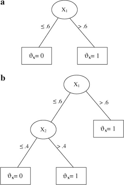
True tree structure in the simulation. a (top): Model 1a; 5b (bottom): Model 1b.

Model 1a was successfully identified by “party” (tree plot in Figure 6a), with the split of X₁ at .572 slightly off .6 due to random error. “rpart” returned a tree (Figure 6b) that was much larger than necessary, but we noted that the first split (0.617) was correct. The likelihood, log-rank, adaptive normalization, and global normalization methods had similar problems—they were able to correctly find the first split but the tree size was excessively large even after pruning (the problem of “overfit”). The Gordon–Olshen method failed to find the correct first split.

Figure 6.

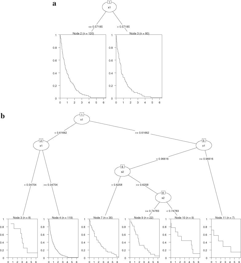
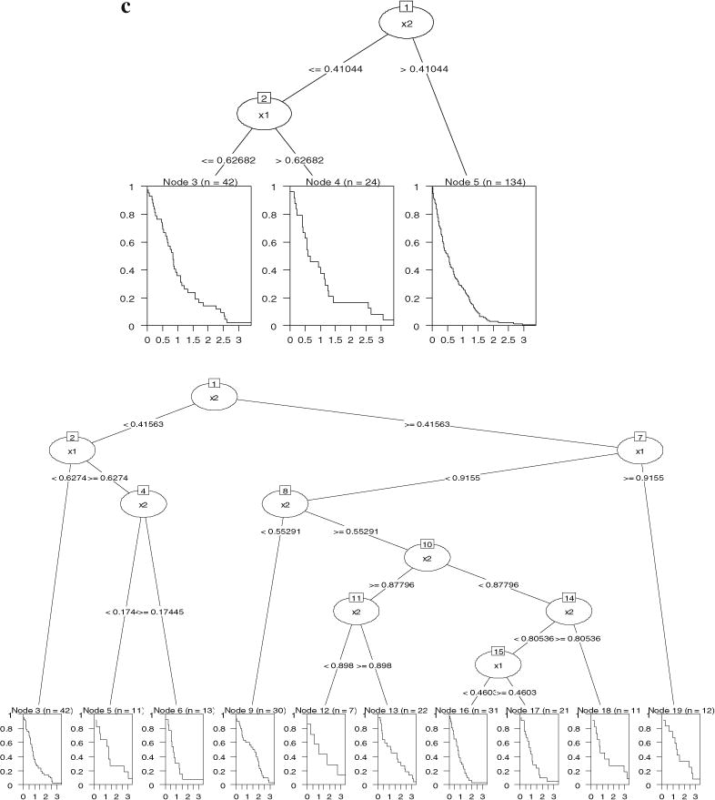
Survival tree results for simulated Model 1a and Model 1b. 6a (top): “party” results for Model 1a; 6b (bottom): “rpart” results for Model 1a; 6c (top): “party” results for Model 1b; 6d (bottom): “rpart” results for Model 1b.

For Model 1b where two splits existed in the tree, “party” split the data correctly (see Figure 6c) though the order of the splitting variables was different from that in Figure 5b. Note that the hazard parameter ϑ_x was zero for the covariate space where X₁ ≤ 0.6 and X₂ ≤ 0.4, and one for the rest. Both trees reflected this partition. “rpart” identified the covariate space where ϑ_x was zero but the problem of overfitting remained (Figure 6d). The same problem occurred with the likelihood, Gordon–Olshen, adaptive normalization, global normalization, and the log-rank methods, with all producing extra unnecessary splits.

These two simple experiments show that conditional inference survival tree implemented in “party” outperforms the other survival tree algorithms—the major problem of which lies in the ineffectiveness of tree pruning, and this problem can lead to overfitting and false interpretation of data. However, this does not deny the value of these methods, as to be discussed later, in survival ensembles that aggregate over single fully-grown survival trees (i.e., without pruning).

4. Bagging for Survival Data

In addressing the problem of instability for single trees (Berk, 2008; Strobl et al., 2009), the general principle of bagging is appealing for survival contexts as well, but the procedure needs some technical adjustment. Hothorn et al. (2004) proposed a method of bagging survival trees. In contrast to averaging over point values in classification (majority voting in a terminal node) or regression (mean response in a terminal node) problems, they use conditional survival probability functions as predicted outcomes. Specifically, for a new observation, the estimate of its survival probability function is based on observations with “close” covariate values, that is, observations which are elements of the same leaf of a survival tree as the new observation itself. A single Kaplan–Meier curve is then computed based on “close” observations aggregated from all bootstrap samples, as the estimated outcome for the new observation. “rpart” was used for constructing survival trees, but it was suggested that arbitrary tree growing algorithm can be used for this bagging procedure (Hothorn et al. 2004).

Hothorn et al. (2004) used integrated Brier score (Graf et al., 1999) as the index of goodness of prediction. They showed via simulation that bagged survival trees improved upon single survival trees in terms of prediction accuracy, and the improvement was more substantial with less censoring. They also demonstrated that the prediction performance of bagging was hardly affected when the number of non-informative covariates increased, suggesting its robustness against noise in the data.

4.1. Available Computer Software

A function in the “party” package cforest() implements bagging survival trees, and one just needs to fix the number of variables evaluated et each node (mtry argument) to the number of available predictors. This bagging procedure has also been implemented in an R package “ipred” (Peters, Hothorn, Ripley, Therneau, & Atkinson, 2009). Users can choose the number of bootstrap samples to be drawn (i.e., the number of trees). Alternative sampling methods other than bootstrap sampling are available. Kaplan–Meier estimates can be obtained for new observations. In practical applications, Brier scores will vary from trial to trial because of the random sampling involved in the bagging procedure. By examining how close the results are across trials, users can get a sense of to what extent the stability has been reached, and decide if more trees are needed.

5. Random Forests for Survival Data

The random forests algorithm has been adapted to the survival responses by Breiman (2002, 2003a, 2003b), Hothorn, Bühlmann, Dudoit, Molinaro, and van der Laan (2006a), and Ishwaran et al. (2008).

Breiman (2002, 2003a, 2003b) developed what he called “survival forests” in his last years of work. In constructing survival trees, unlike all the other algorithms, he partitioned the time-covariate space instead of just the covariate space. In particular, there is a probability of .75 to split to time and a probability of .25 to split on one of the covariates. In a time split of a node, all cases in the original node are in each child node. The splitting criterion is to increase the observed data log-likelihood assuming a constant hazards model within each node. Trees are grown until each terminal node has exactly one uncensored observation in it. The predicted value is the survival probability function. Breiman (2002) demonstrated that this procedure was superior to the Cox regression in various datasets, especially in situations where the Cox regression ignored the predictors which were only relevant within a limited time period (a violation of the proportional hazards assumption). However, he also pointed out that this method “is still being born and needs more testing, working with, and extending” (Breiman, 2002).

Hothorn et al. (2006a) proposed a random forest algorithm for survival data using a weighting scheme. Observations are weighted by the inverse probability of censoring (IPC) weights, which defines the probability for an observation to be selected in the bootstrapping sampling. This is a similar idea as used in Molinaro et al.’s (2004) survival tree algorithm. The predicted value is a weighted average of log survival time, so residual sum of squares can be used to measure prediction error. The performance of this method seems to depend on the censoring rate. The method can be problematic in cases where the censoring rate is high (shown by Ishwaran et al., 2008), probably because, by definition, the weights are zero for censored observations, meaning censored observations are not used at all in constructing trees. However, it seems to work well when most of the events are observed (shown by Hothorn et al. 2006a).

Ishwaran et al. (2008) developed a “random survival forests” method that adapts the standard random forests (Breiman, 2003a, 2003b) to survival responses. Four alternative splitting rules are available in constructing survival trees: log-rank splitting, conversation-of-events principle, log-rank score (standardized log-rank statistic) splitting, and random log-rank splitting (Ishwaran et al., 2008). Trees are grown to full size under the constraint that a terminal node should have at least one death. The predicted value is mortality, derived from the cumulative hazard function (CHF). Harrell’s concordance index (C-index; Harrell et al., 1982) is used as the measure of prediction performance. Like the standard random forests, a variable importance measure can be calculated for each predictor, which is defined as the original prediction error subtracted from the prediction error obtained by randomization the values in that predictor, given that the forest is unchanged. In application to empirical datasets (Ishwaran et al., 2008), this method has been shown to be robust against censoring and robust against noise variables in the data.

5.1. Available Computer Software

The survival forests algorithm by Breiman (2002) is provided on his website (http://www.stat.berkeley.edu/~breiman/sf.html), as free software written in Fortran 77. It has not been embedded in the more user-friendly commercial software with his other data mining techniques. The forest algorithm by Hothorn et al. (2006a) does not seem to have been implemented in publicly available programs. The random survival forests algorithm is implemented in the R package “randomSurvivalForest” (Ishwaran & Kogalur, 2010). Users can choose one of the four splitting rules in growing survival trees, and can choose the values for “ntree” (the number of trees) and “mtry” (the number of covariates randomly selected for each split). The calculation of variable importance is available, and there is also an imputation procedure for handling missing data as described in Ishwaran et al. (2008).

6. Evaluating Survival Tree, Bagging and Random Survival Forests

Next we compare four methods: (a) Cox regression, (b) bagging survival trees (Hothorn et al., 2004), (c) random survival forests (Ishwaran et al., 2008), and (d) conditional inference survival tree (Hothorn et al., 2006b), via simulated data where the censoring rate was manipulated at different levels.

Survival times were simulated in the same way as the previous setup, but here censoring rates were controlled to be approximately 25, 50, and 75 %. We assumed that observation times were distributed uniformly on [0, γ ]. For any observation, if the observation time was shorter than the survival time, the outcome was censored. Values of the censoring parameter γ used in each trial are listed in Table 3.

Table 3.

Values of the censoring parameter γ used in the simulation.

Set	Censoring rate
	25 %	50 %	75 %
2a	2.0	.65	.17
2b	.55	.16	.05

Similar to the previous setup, two independent predictors X₁ and X₂ were uniformly distributed on [0, 1]. The sample size was N = 200. The true models were:

$${\vartheta }_{\mathrm{x}}=X_{1}I(X_1\le .7)+3X_{1}I(X_1>.7);$$ 2a

$${\vartheta }_{\mathrm{x}}=3X_1+X_2+X_1{X}_2.$$ 2b

Model 2a is a spline regression in which X₁’s effect is three times as strong when it exceeds the value of .7. Model 2b includes main effects for both covariates as well as interaction. In fitting the Cox regression, X₁, X₂ and their product term were examined. One hundred bootstrap samples were drawn in each bagging procedure. For random survival forests, we chose the log-rank splitting rule to grow survival trees. Five hundred trees were grown for each forest, and one variable was randomly selected for each split. Results are presented in Table 4.

Table 4.

Results from Cox regression, bagging, and random survival forests in the simulation.

	Cox regression Parameter estimate (SE)	Bagging OOB Brier’s score	Random survival forests Variable importance
2a
25 % censoring		With both = .1522	Error rate = 32.31 %
X1	3.56 (.70)	.1892	.2014
X2	.51 (.68)	.147	−.0110
X1X2	−.94 (1.14)	–	–
50 % censoring		With both = .1696	Error rate = 28.86 %
X1	2.90 (.89)	.2357	.2416
X2	−1.36 (1.02)	.1664	.0079
X1X2	1.64 (1.49)	–	–
75 % censoring		With both = .1306	Error rate = 30.39 %
X	5.38 (1.38)	.1998	.3224
X2	1.51 (1.64)	.1236	−.0246
X1X2	−2.28 (2.16)	–	–
2b
25 % censoring		With both = .1069	Error rate = 24.65 %
X1	3.86 (.72)	.1719	.1436
X2	1.79 (.71)	.1336	.0221
X1X2	.31 (1.07)	–	–
50 % censoring		With both = .1533	Error rate = 26.88 %
X1	2.81 (.90)	.2127	.1849
X2	.08 (.98)	.1572	.0015
X1X2	1.65 (1.43)	–	–
75 % censoring		With both = .1476	Error rate = 29.58 %
X1	2.43 (1.43)	.186	.1258
X2	.78 (1.54)	.1483	.0117
X1X2	1.31 (2.13)	–	–

OOB Brier’s scores shown in the table are prediction errors of the bagging procedure without the covariate.

For Model 2a, Cox regression identified X₁ as the only significant predictor at all three levels of censoring. But the effect of X₁ was over estimated, especially when the censoring rate was high (75 %). This is not hard to explain, because the censored observations were more of those with lower hazard—in the current setting, those with lower X₁ values. In the absence of these observations, the estimate for X₁ coefficient tended to be biased toward the higher side. Bagging showed that removing X₁ resulted in a higher error rate at all censoring levels, while removing X₂ slightly lowered the error rate. Thus bagging correctly reflected the importance of X₁ and triviality of X₂in predicting the survival outcome, and the effectiveness of the method did not seem to be affected by censoring rate. Random survival forests were similarly successful, and the overall prediction error of the forest was not affected by censoring.

For Model 2b, Cox regression did not have enough power to detect the interaction, and, as the censoring rate increased, the two main effects became insignificant as well. In contrast, bagging showed that prediction error went up by removing either predictor, suggesting that they were both predictive of the outcome. For the weaker predictor X₂, the change in prediction error became very small when censoring rate reached 50 % or higher. Similarly, random survival forests showed that the variable importance measure was large for X₁ at all times, but very small for X₂ at the 50 and 75 % censoring level. The overall prediction error tended to go up as the censoring rate increased.

With regard to the tree results, survival trees seemed to be sensitive to the shift in regression coefficient in Model 2a—all of them found a split around .7 (see Figure 7a–c). For Model 2b, trees detected the interaction at all three censoring levels (Figure 7d–f), though the number of splits decreases as the censoring rate increases.

Figure 7.

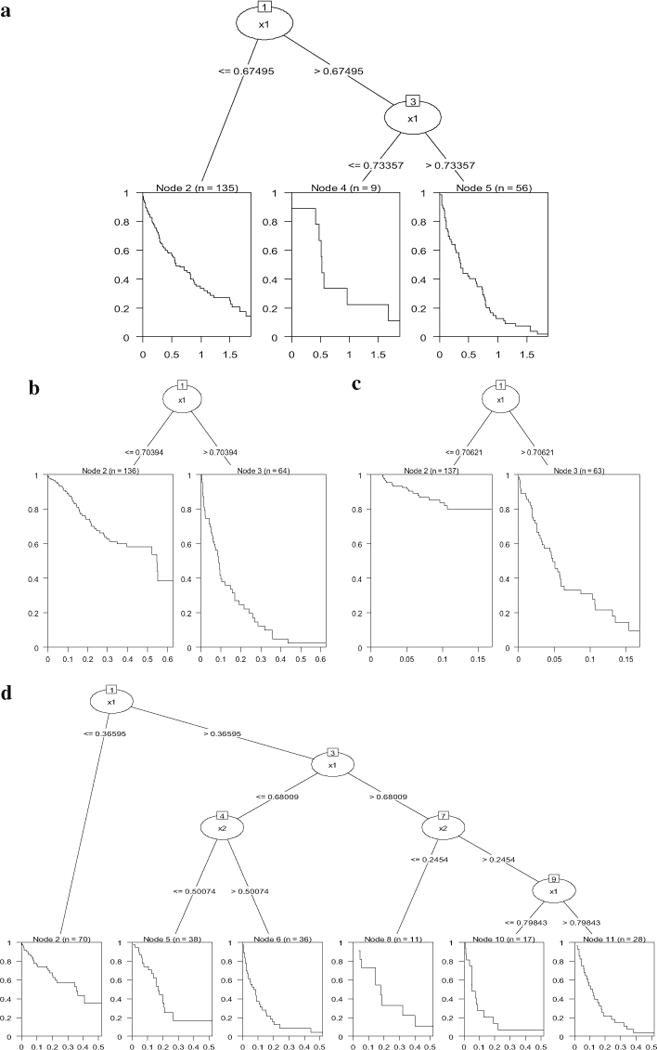
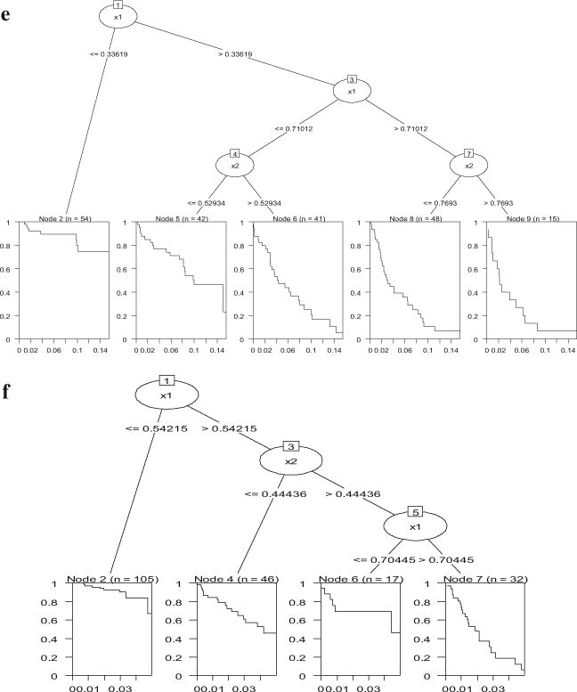
Conditional inference survival trees for simulated Model 2a and Model 2b. 7a (top): Model 2a, 25 % censoring; 7b (bottom left): Model 2a, 50 % censoring; 7c (bottom right): Model 2a, 75 % censoring; 7d (top): Model 2b, 25 % censoring; 7e (bottom): Model 2b, 50 % censoring; 7f: Model 2b, 75 % censoring.

In sum, the simulations show two situations where Cox regression can be problematic: (a) it can be biased when censoring is related to the explanatory variables, and (b) statistical power is substantially affected by high censoring rate. In contrast, bagging and random survival forests seem to be less affected by censoring. Survival trees can be helpful in terms of detecting shifts in nonlinear relations as well as detecting interactions.

6.1. Recidivism Example Revisited

We can then return to recidivism data and reconsider the results obtained by different methods. The first confusion is about the effect of AGE, which was suggested to be an important predictor by all methods except bagging. A possible explanation is that the performance of bagging was affected by censoring (45 % in the recidivism data), considering the simulation for Model 2b that the effect of X₂ could hardly be detected when the censoring rate was 50 or 75 %. The decrease in prediction error by removing AGE might be a result of random sampling embedded in the bagging procedure. For the Cox regression, there did not seem to be evidence for obvious violation of the model assumption (i.e., proportional hazards; see Figure 1), so we can believe the results from Cox regression are reliable. In addition, random survival forest also identified AGE as the most important predictor; in the survival tree, AGE was the first variable to split. So we can conclude that AGE did have an effect on the hazard of re-arrest, and the results produced by bagging seemed to be misleading in this example.

We showed via simulation that, with similar sample size (N = 200) and similar censoring rate (50 %), Cox regression might not have enough power to detect an interaction. Survival tree suggested an interaction in the recidivism example, but given its exploratory nature, such a conclusion cannot be reached here. Similarly, it is possible that the effect of AGE was nonlinear. These clues from exploratory data mining can be examined in future research.

7. Discussion

7.1. Review of Existing Methods

Among the survival tree algorithms, the conditional inference survival tree developed by Hothorn et al. (2006b) seems to be more reliable and less likely to overfit, and this seems to be a major problem for the other survival tree algorithms. However, for survival ensemble methods whose major goal is forecasting, the overfitting problem of most survival tree algorithms becomes less important, because the ensemble methods used here usually aggregate over large trees (or unpruned trees). The choice of survival tree algorithms for ensemble methods does not seem to have been specifically examined, except for the random survival forests by Ishwaran et al. (2008), who showed four alternative tree splitting rules were all fairly good.

The survival ensemble methods are only recently proposed and still in the development stage. In addition to the methods reviewed above, Hothorn et al. (2006a) also developed a generic gradient boosting algorithm, inspired by another powerful statistical learning device boosting (Schapire, 1999). They have only been tested with a limited number of simulations and practical datasets, and potential flaws are possibly still uncovered. For example, in the recidivism example, interpretation of the covariate AGE would be misleading based on the bagging method (Hothorn et al., 2004). In a real substantive application (Zhou, Kadlec, & McArdle, 2014), the authors found a situation where the random survival forests (Ishwaran et al., 2008) seemed to fail—i.e., when there was only one predictor with two categories. There may be certain conditions under which these methods perform well, and certain conditions under which these methods meet their limits. These are still unclear for now, and need more investigation in the future. In addition, ambiguities exist such as how big the variable importance value should be to be judged as a meaningful predictor. Strobl et al. (2009) suggested a conservative strategy to only include predictors whose importance scores exceed the amplitude of the largest negative scores, while Ishwaran et al. (2008) added noise variables to the dataset and used them as reference variables. This also needs further investigation.

7.2. Suggestions for Practical Use

Proper interpretation of the results is the key in using survival tree methods. Due to the relative immaturity of these methods, it seems important for users to have the basic knowledge of these procedures. Being aware of their drawbacks and limitations can avoid making misleading statements. This is not to discourage the use of survival trees and ensembles—instead we recommend their use, but in combination with other conventional methods. Cox regression is very popular in the analysis of survival data, but it is limited in various situations (Breiman, 2002), and in practice often used without rigor (i.e., the proportional hazard assumption not being carefully examined). On the other hand, we should not be too optimistic about data mining. As shown by Ishwaran et al. (2008), with some datasets, prediction accuracy of the exploratory methods were not better than the Cox regression, which suggests that the superiority of these methods is not always seen, but only in situations when the conventional methods meet their limits. But it never hurts to use them as supplemental tools, with which one may obtain extra information in the data that are not grasped by conventional survival analysis.

There are several conditions under which survival forests can be especially informative. First, the most typical case is when we have a large number of predictors and a small sample size, and the Cox regression is limited by low statistical power. Furthermore, if no clear theory or hypothesis is available for testing only a few specific covariates, it seems impractical to include all main effects as well as higher-order interaction terms in the model. In contrast, survival forests is free from the limit of statistical power and has an advantage in detecting interactions. Second, Ishwaran et al. (2008) showed that the prediction error of the Cox regression increased as the number of uncorrelated covariates became larger, whereas the random forests was robust against noise variables in the data. Third, in cases where the proportional hazard assumption is violated, for instance, when the effect of a relevant predictor only exists for a limited time period, this predictor is likely to be ignored (Breiman, 2002) by the Cox regression. Survival trees are insensitive to the proportional hazard assumption (unless the splitting rule is based on the assumption). Four, the performance of the Cox regression is dependent on the censoring rate. We found that in cases where the censoring rate was high, the Cox regression could yield biased results when the predictors were responsible for censoring. Censoring could also substantially affect the statistical power of the Cox regression. Random forests seems to be less affected by the censoring rate.

These statistical learning techniques are at their best when the goal is forecasting. They can respond to data features which are likely to be missed by other conventional methods, but these features are only reflected in the improved prediction accuracy. These methods are like a black box when the question is how the predictors are related to the outcome. Also note that the conclusions drawn from these exploratory methods are not supported on a probability basis, which, as the fundamental of a hypothesis testing paradigm, is still a core scientific element in the field. If the research question is to formally demonstrate the relation of a predictor to the outcome, that is, test a specific a priori theory, these methods are no substitute for long established, testable models.

References

- Berk RA. Statistical learning from a regression perspective. New York, NY: Springer; 2008. [Google Scholar]
- Breiman L. Bagging predictors. Machine Learning. 1996;24:123–140. [Google Scholar]
- Breiman L. Random forests. Machine Learning. 2001;45:5–32. [Google Scholar]
- Breiman L. Software for the masses. Department of Statistics, University of California; Berkeley: 2002. Retrieved from http://www.stat.berkeley.edu/~breiman/wald2002-3.pdf. Accessed 1 July, 2014. [Google Scholar]
- Breiman L. How to use survival forests. Department of Statistics, University of California; Berkeley: 2003a. Retrieved from http://www.stat.berkeley.edu/~breiman/SF_Manual.pdf. Accessed 1 July, 2014. [Google Scholar]
- Breiman L. Manual—setting up, using and understanding random forests V4.0. 2003b Retrieved from http://www.stat.berkeley.edu/~breiman/Using_random_forests_v4.0.pdf. Accessed 1 July, 2014.
- Breiman L, Friedman JH, Olshen R, Stone CJ. Classification and regression trees. New York, NY: Chapman & Hall; 1984. [Google Scholar]
- Butler J, Gilpin E, Gordon L, Olshen R. Tree-structured survival analysis II. Department of Biostatistics, Stanford University; 1989. (Technical report). [Google Scholar]
- Ciampi A, Thiffault J, Nakache JP, Asselain B. Stratification by stepwise regression, correspondence analysis and recursive partition: A comparison of three methods of analysis for survival data with covariates. Computational Statistics & Data Analysis. 1986;4:185–204. [Google Scholar]
- Cox DR. Regression models and life tables. Journal of the Royal Statistical Society Series B. 1972;34(2):187–220. [Google Scholar]
- Cox DR, Oakes D. Analysis of survival data. London: Chapman & Hall; 1984. [Google Scholar]
- Davis R, Anderson J. Exponential survival trees. Statistics in Medicine. 1989;8:947–961. doi: 10.1002/sim.4780080806. [DOI] [PubMed] [Google Scholar]
- DeWit DJ, Adlaf EM, Offord DR, Ogborne AC. Age at first alcohol use: A risk factor for the development of alcohol disorders. American Journal of Psychiatry. 2000;157(5):745–750. doi: 10.1176/appi.ajp.157.5.745. [DOI] [PubMed] [Google Scholar]
- Gordon L, Olshen RA. Tree-structured survival analysis. Cancer Treatment Reports. 1985;69:1065–1069. [PubMed] [Google Scholar]
- Graf E, Schmoor C, Sauerbrei W, Schumacher M. Assessment and comparison of prognostic classification schemes for survival data. Statistics in Medicine. 1999;18:2529–2545. doi: 10.1002/(sici)1097-0258(19990915/30)18:17/18<2529::aid-sim274>3.0.co;2-5. [DOI] [PubMed] [Google Scholar]
- Harrell F, Califf R, Pryor D, Lee K, Rosati R. Evaluating the yield of medical tests. Journal of the American Medical Association. 1982;247:2543–2546. [PubMed] [Google Scholar]
- Henning KR, Frueh BC. Cognitive-behavioral treatment of incarcerated offenders: An evaluation of the Vermont Department of Corrections’ cognitive self-change program. Criminal Justice and Behavior. 1996;23:523–541. [Google Scholar]
- Hothorn T, Bühlmann P, Dudoit S, Molinaro A, van der Laan MJ. Survival ensembles. Biostatistics. 2006a;7(3):355–373. doi: 10.1093/biostatistics/kxj011. [DOI] [PubMed] [Google Scholar]
- Hothorn T, Hornik K, Strobl C, Zeileis A. Package ‘party’: A laboratory for recursive part(y)itioning (R package Version 0.9-9997) [Computer software] 2010 Retrieved from http://cran.r-project.org/web/packages/party/index.html. Accessed 15 Oct, 2010.
- Hothorn T, Hornik K, Zeileis A. Unbiased recursive partitioning: A conditional inference framework. Journal of Computational and Graphical Statistics. 2006b;15:651–674. [Google Scholar]
- Hothorn T, Lausen B, Benner A, Radespiel-Tröger M. Bagging survival trees. Statistics in Medicine. 2004;23:77–91. doi: 10.1002/sim.1593. [DOI] [PubMed] [Google Scholar]
- Hothorn T, Zeileis A. Package ‘partykit’: A Toolkit for Recursive Partytioning (R package Version 0.1-6) [Computer software] 2012 Retrieved from http://cran.r-project.org/web/packages/partykit/index.html. Accessed 3 Sept, 2013.
- Intrator O, Kooperberg C. Trees and splines in survival analysis. Statistical Methods in Medical Research. 1995;4(3):237–261. doi: 10.1177/096228029500400305. [DOI] [PubMed] [Google Scholar]
- Ishwaran H, Kogalur UB. Package ‘randomSurvivalForest’: Random survival forest. (R package Version 3.6.3) [Computer Software] 2010 Retrieved from http://cran.r-project.org/web/packages/randomSurvivalForest/index.html. Accessed 15 Oct, 2010.
- Ishwaran H, Kogalur UB, Blackstone EH, Lauer MS. Random survival forests. The Annals of Applied Statistics. 2008;2(3):841–860. [Google Scholar]
- Keleş S, Segal MR. Residual-based tree structured survival analysis. Statistics in Medicine. 2002;21:313–326. doi: 10.1002/sim.981. [DOI] [PubMed] [Google Scholar]
- LeBlanc M, Crowley J. Relative risk trees for censored survival data. Biometrics. 1992;48:411–425. [PubMed] [Google Scholar]
- LeBlanc M, Crowley J. Survival trees by goodness of split. Journal of the American Statistical Association. 1993;88:457–467. [Google Scholar]
- Mantel N. Evaluation of survival data and two new rank order statistics arising in its consideration. Cancer Chemotherapy Reports. 1966;50(3):163–170. [PubMed] [Google Scholar]
- Mertens JR, Kline-Simon AH, Delucchi KL, Moore C, Weisner CM. Ten-year stability of remission in private alcohol and drug outpatient treatment: Non-problem users versus abstainers. Drug and Alcohol Dependence. 2012;125(1):67–74. doi: 10.1016/j.drugalcdep.2012.03.020. [DOI] [PMC free article] [PubMed] [Google Scholar]
- McArdle JJ. Exploratory data mining using CART in the behavioral sciences. In: Cooper H, Camic P, Long D, Panter AT, Rindskopf D, Sher K, editors. APA handbook of research methods in psychology. Washington, DC: The American Psychological Association; 2011. [Google Scholar]
- Molinaro AM, Dudoit S, van der Laan MJ. Tree-based multivariate regression and density estimation with right-censored data. Journal of Multivariate Analysis. 2004;90:154–177. [Google Scholar]
- Morgan JN, Sonquist JA. Problems in the analysis of survey data, and a proposal. Journal of the American Statistical Association. 1963;58:415–434. [Google Scholar]
- Morita JG, Lee TW, Mowday RT. The regression-analog to survival analysis: A selected application to turnover research. Academy of Management Journal. 1993;36(6):1430–1464. [Google Scholar]
- Peters A, Hothorn T, Ripley BD, Therneau T, Atkinson B. Package ‘ipred’: Improved Predictors. (R package Version 0.9-3) [Computer Software] 2009 Retrieved from http://cran.r-project.org/web/packages/ipred/index.html. Accessed 1 July, 2014.
- Peto R, Peto J. Asymptotically efficient rank invariant test procedures. Journal of the Royal Statistical Society Series A. 1972;135(2):185–207. [Google Scholar]
- Schemper M, Stare J. Explained variation in survival analysis. Statistics in Medicine. 1996;15:1999–2012. doi: 10.1002/(SICI)1097-0258(19961015)15:19<1999::AID-SIM353>3.0.CO;2-D. [DOI] [PubMed] [Google Scholar]
- Segal MR. Regression trees for censored data. Biometrics. 1988;44:35–47. [Google Scholar]
- Schapire RE. A brief introduction to boosting. Proceedings of the Sixteenth International Joint Conference on Artificial Intelligence (IJCAI 99) 1999:1401–1405. [Google Scholar]
- Singer JD, Willett JB. Modeling the days of our lives: Using survival analysis when designing and analyzing longitudinal studies of duration and the timing of events. Psychological Bulletin. 1991;110(2):268. [Google Scholar]
- Singer JD, Willett JB. Applied longitudinal data analysis. New York, NY: Oxford; 2003. [Google Scholar]
- Stone M. Choice and assessment of statistical predictions. Journal of the Royal Statistical Society Series B. 1974;36:111–133. [Google Scholar]
- Strobl C, Malley J, Tutz G. An introduction to recursive partitioning: Rational, application, and characteristics of classification and regression trees, bagging, and random forests. Psychological Methods. 2009;14(4):323–348. doi: 10.1037/a0016973. [DOI] [PMC free article] [PubMed] [Google Scholar]
- Therneau TM, Atkinson B. Package ‘rpart’: Recursive partitioning (R package Version 3.1-48) [Computer software] 2010 Retrieved from http://cran.r-project.org/web/packages/rpart/index.html. Accessed 15 Oct, 2010.
- Therneau TM, Grambsch PM, Fleming TR. Martingale-based residuals for survival models. Biometrika. 1990;77(1):147–160. [Google Scholar]
- Zhang HP, Singer B. Recursive partitioning in the health sciences. New York, NY: Springer; 1999. [Google Scholar]
- Zhou Y, Kadlec KM, McArdle JJ. Predicting mortality from demographics and specific cognitive abilities in the Hawaii Family Study of Cognition. In: McArdle JJ, Ritschard G, editors. Contemporary issues in exploratory data mining. New York, NY: Routledge; 2014. pp. 429–449. [Google Scholar]
- Zosuls KM, Ruble DN, Tamis-LeMonda CS, Shrout PE, Bornstein MH, Greulich FK. The acquisition of gender labels in infancy: Implications for gender-typed play. Developmental Psychology. 2009;45(3):688. doi: 10.1037/a0014053. [DOI] [PMC free article] [PubMed] [Google Scholar]
Associated Data
This section collects any data citations, data availability statements, or supplementary materials included in this article.