A Bayesian framework for de novo mutation calling in parents-offspring trios

Abstract

Motivation: Spontaneous (de novo) mutations play an important role in the disease etiology of a range of complex diseases. Identifying de novo mutations (DNMs) in sporadic cases provides an effective strategy to find genes or genomic regions implicated in the genetics of disease. High-throughput next-generation sequencing enables genome- or exome-wide detection of DNMs by sequencing parents-proband trios. It is challenging to sift true mutations through massive amount of noise due to sequencing error and alignment artifacts. One of the critical limitations of existing methods is that for all genomic regions the same pre-specified mutation rate is assumed, which has a significant impact on the DNM calling accuracy.

Results: In this study, we developed and implemented a novel Bayesian framework for DNM calling in trios (TrioDeNovo), which overcomes these limitations by disentangling prior mutation rates from evaluation of the likelihood of the data so that flexible priors can be adjusted post-hoc at different genomic sites. Through extensively simulations and application to real data we showed that this new method has improved sensitivity and specificity over existing methods, and provides a flexible framework to further improve the efficiency by incorporating proper priors. The accuracy is further improved using effective filtering based on sequence alignment characteristics.

Availability and implementation: The C++ source code implementing TrioDeNovo is freely available at https://medschool.vanderbilt.edu/cgg.

Contact: bingshan.li@vanderbilt.edu

Supplementary information: Supplementary data are available at Bioinformatics online.

1 Introduction

Traditional research in the field of genetics for human complex disease has focused largely on inherited variation. For sporadic cases without family history, it is well known that de novo copy number variants are implicated in autism (Levy et al., 2011; Sebat et al., 2007) and other psychiatric disease (Hehir-Kwa et al., 2011; Maiti et al., 2011). Cost-effective next-generation sequencing (NGS) technologies enable the identification of mutations at base-pair resolution, and a flurry of recent studies revealed important roles of de novo point mutations in the genetic etiology of complex disease, including autism spectrum disorders (Iossifov et al., 2012; Neale et al., 2012; O'Roak et al., 2011, 2012; Ronemus et al., 2014; Sanders et al., 2012), intellectual disability (Gregor et al., 2013; Vissers et al., 2010), schizophrenia (Fromer et al., 2014; Gauthier et al., 2010; Gulsuner et al., 2013). These findings showed promise of sequencing sporadic parents-proband trios for genetics studies of human disease. Since de novo mutations (DNMs) have not been subject to strong purifying selection, causal mutations are expected to have large effects, enabling effective identification of causal genes or pathways from a drastically reduced number of candidates. We envision that this strategy will continuously be used as an effective alternative to classical genetic studies to identify genetic factors through both exome and whole genome sequencing.

A critical step in such studies is to accurately call DNMs from sequencing. This is challenging due to sequencing error and alignment artifacts, which predominately outnumber true mutations. It is therefore important to develop methods that can effectively sift real mutations through massive amount of noise. Standard approaches infer genotypes for each individual separately in a trio, usually using GATK (DePristo et al., 2011; McKenna et al., 2010) or Samtools (Li et al., 2009), and identify putative DNMs by comparing proband’s and parental genotypes. More efficient joint calling methods have been developed, including PolyMutt (Li et al., 2012) & DeNovoGear (Ramu et al., 2013), and were shown to outperform standard approaches dramatically. A major limitation of these joint-calling methods is the entanglement of DNMs with Mendelian inheritance in the same model such that the joint likelihood of the data depends on the pre-specified mutation rate, resulting in several unappealing consequences. First, it requires specifying a prior mutation rate, which has strong influence on the mutation calling (Ramu et al., 2013), and therefore can result in loss of accuracy when inappropriate mutation rates are used. Second, it is well known that mutation rates vary widely across the genome, and therefore any single pre-specified mutation rate is not optimal. Third, the estimates for complex mutations, such as short insertion and deletion (Indel) and structural variations, are largely unknown, and an inappropriate rate may result in dramatically reduced mutation calling efficiency. Lastly, the evidence of mutations reported by these callers has a less intuitive interpretation because of the entanglement of the pre-specified mutation rate in the data likelihood calculation.

To overcome these limitations, we developed a new de novo calling algorithm, TrioDeNovo, which is a Bayesian framework that evaluates evidence of DNM mainly based on the data and adjusts post-hoc the effect of mutation rates on the calling through prior odds. This is achieved through a Bayesian model selection approach, in which it calculates the Bayes Factor (BF) of two models, namely M₁ that the offspring harbors at least one mutation in the two alleles, and M₀ that the offspring’s genotype follows Mendelian transmission. This approach of calculating de novo evidence (i.e. BF) avoids the need for accurate specification of prior mutation rates and has a natural interpretation as the relative likelihood of data under two competing and mutually exclusive models. After evaluating BF, flexible prior mutation rates can be adjusted post-hoc to get posterior odds of DNMs for different sites and different mutation types according to prior knowledge. Through extensively simulations and real datasets, we showed that the new framework improves sensitivity and specificity over existing methods in detection of DNMs, especially for moderate depth of coverage (e.g. 20×). Coupled with our recently developed method for effective filtering of alignment artifacts, we hope that this new framework is useful to the research community for accurate DNM calling to facilitate the identification of genetic factors for human disease.

2 Methods

2.1 DNM calling algorithm

TrioDeNovo uses a Bayesian model selection framework for DNM calling. The input to TrioDeNovo is a variant calling format (VCF) (Danecek et al., 2011) file, which can be generated using widely used tools such as GATK (DePristo et al., 2011; McKenna et al., 2010) and Samtools (Li et al., 2009). TrioDeNovo extracts genotype likelihood (GL) values stored in the VCF file for mutation modeling. GL is defined as the probability of observing aligned reads, denoted as R, at a specific position given a specific underlying genotype G, i.e. P(R|G). The basic idea is to consider all bases aligned at a specific position on the genome as a series of Bernoulli trials, each with an empirically calibrated error rate specifying the probability that the observed base is different from the true allele. The simplest calculation of the GL assumes that sequencing errors are independent and more sophisticated error models incorporate inter-dependency of sequencing errors (see Li et al., 2009, 2012 for details). The benefit of utilizing pre-calculated GL values stored in VCF files is to take advantage of accurate GL values generated by highly specialized tools such as GATK and Samtools. It is standard for state-of-the-art variant calling methods to output GLs in VCF files and therefore TrioDeNovo can continue to benefit from the improvement made to the GL calculation by these specialized tools.

For each site in the sequence data, we define two models, M₁, which represents the model that there is at least one mutation in the offspring, and M₀, which specifies the model that the genotypes of the parent-offspring trio are consistent with Mendelian transmission law. Define an allelic mutation model, κ, as a matrix of relative probabilities from parental alleles to mutant alleles, conditional on that a mutation occurred. A simple model for single nucleotide variant (SNV) mutations is illustrated in the matrix below.

$$\begin{array}{l}\begin{array}{cccc} \mathbf{A} & \mathbf{C}& \mathbf{G} & \mathbf{T}\end{array}\\ \begin{array}{c}A\\ C\\ G\\ T\end{array}\left[\begin{array}{cccc}& \upsilon & \omega & \upsilon \\ \upsilon & & \upsilon & \omega \\ \omega & \upsilon & & \upsilon \\ \upsilon & \omega & \upsilon & \end{array}\right]\end{array}$$

In this simplified model mutations are symmetric, all transitions have the same mutation rate ($\omega$) as well as transversions ($\upsilon$), and $2\upsilon +\omega =1$. Given a mutation rate, denoted as μ and assumed to be the same for all parental alleles, the absolute allelic mutation rates can be calculated by multiplying μ in the above matrix. Other flexible mutation models can be provided to TrioDeNovo by the user if desired. In the allelic mutation model only one parameter is free and we let the transition $\omega$ be the parameter of the model.

Let R denote the aligned reads at a genome position for all individuals in a trio. The goal is to calculate the posterior odds of the two models, given R and κ, as the following:

$$\frac{P\left(M_1\text{|}\mathit{R}\right)}{P\left(M_0\text{|}\mathit{R}\right)}=\frac{P\left(\mathit{R}\text{|}{M}_1\right)}{P\left(\mathit{R}\text{|}{M}_0\right)}\times \frac{P(M_1)}{P(M_0)}$$

In the above, $\frac{P\left(\mathit{R}\text{|}{M}_1\right)}{P\left(\mathit{R}\text{|}{M}_0\right)}$ is the BF of the two models, and $\frac{P(M_1)}{P(M_0)}$ is the prior odds of the two models. A confident DNM is called when the posterior odds is greater than a threshold, e.g. 1, indicating that mutations are more likely than Mendelian transmission, a posterior. Another way is to rank the candidates according to the posterior odds and select the top candidates for further evaluation. In TrioDeNovo, instead of reporting the posterior odds, which depends on both BF and prior odds, we define de novo quality (DQ) based on the BF only, i.e., $\text{DQ}={\log }_{10}\left(\frac{P\left(\mathit{R}\text{|}{M}_1\right)}{P\left(\mathit{R}\text{|}{M}_0\right)}\right)$. The benefit of this strategy is that TrioDeNovo concentrates on model evaluation, which is essentially unaffected by the prior mutation rate (see below), and the prior odds $\frac{P(M_1)}{P(M_0)}$ can be specified post-hoc so that different priors can be used for different genomic regions. If there is a need to re-adjust the prior for some candidates when better estimates of priors are available this can be easily done without re-calling DNMs. To adjust the prior odds, if we know the estimated mutation rate at a locus, e.g. P(M₁), we can use that to approximate the prior odds as P(M₀) is close to 1. Often times we have the relative estimate of the mutation rate of a particular locus relative to the genome average mutation rate, denoted as P_g(M₁). For example, if a locus is 10 times more (or less) mutable than the genome average, a simple adjustment is to add (or subtract) log₁₀(10) = 1 to (or from) the DQ to get adjusted DQ (DQ_adj). The ranking of the DQ_adj values incorporates the differential prior odds of different genomic loci. The posterior odds are obtained as ${10}^{{\text{DQ}}_{\text{adj}}+{\text{log}}_{10}{P}_g(M_1)}$ when knowledge is available for P_g(M₁). Regardless of the accuracy of P_g(M₁) the order of posterior odds remains the same as long as the relative mutability is properly specified.

The key component of the framework is the calculation of the BF. Let p denote the alternative allele frequency in the population at a specific genomic position, and others be defined as before. BF is calculated as

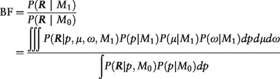In the above we assumed that a priori the allele frequency in parents, the mutation rate and the transition probability are independent. Instead of taking numerical integrations in calculating the BF, we describe our rationales to simplify the model to increase computation efficiency.

2.1.1 Simplification of the prior of parameter p

Given the availability of an extensive catalog of genetic variation with accurate estimates of allele frequencies by the 1000 Genomes Project (1000GP), we can greatly simplify the calculation by considering only a single value in the prior distribution of the allele frequency. At known variant sites we assign $P(p|M_1)$ and $P(p|M_0)$ to 1 for p that equals to the 1000GP estimate and 0 for others. For non-variant sites we assign the corresponding prior probability to 1 for p = 0.001 and to 0 for others; although estimates of actual frequencies are not available, this assignment is expected to be close to true values given that alternative alleles were not observed at these sites in the 1000GP data. This simplification is expected to not only increase the computation speed but also improve the accuracy owing to the comprehensiveness of the current catalog of genetic variation. Let p₀ denote the allele frequency in the 1000GP for known variant sites, and p₀ = 0.001 for others. The BF can be simplified as

$$\text{BF}=\frac{{\displaystyle \int \int P\left(R\text{|}{p}_0,\mu ,\omega ,M_1\right)P(\mu |M_1)P(\omega |M_1)d\mu d\omega }}{P(R|p_0,M_0)}$$ (1)

2.1.2 Simplification of the prior of parameter μ

For a given estimate p = p₀ as above, we calculate $P(R|p_0,\mu ,\omega ,M_1)$ as the following:

$$\begin{array}{l}P\left(R\text{|}{p}_0,\mu ,\omega ,M_1\right)\\ ={\displaystyle \sum }_{G}P\left(R\text{|}G\right)P\text{(}G\text{|}{p}_0,\mu ,\omega ,M_1)\\ ={\displaystyle \sum }_{G_o,G_f,G_m}P\left(R\text{|}G\right)P\left(G_f,G_m\text{|}{p}_0\right)P\text{(}{G}_o\text{|}{G}_f,G_m,\mu ,\omega ,M_1) \end{array}$$ (2)

The term $P\left(R\text{|}G\right)=P(R_o|G_o)P(R_f|G_f)P(R_m|G_m)$ is the product of the GLs of the trio, where R_o, R_f and R_m denote the reads for offspring, father and mother respectively, and similarly G_o, G_f and G_m represent the corresponding genotypes of the trio. $P\left(G_f,G_m\text{|}{p}_0\right)$ is the frequency of the parental genotypes which can be calculated based on the allele frequency $p_0$ assuming Hardy–Weinberg equilibrium, and $P(G_o|G_f,G_m,\mu ,\omega ,M_1)$ is the posterior probability of observing the offspring’s mutant genotype from parental genotype given mutation parameters μ and ω under model M₁. The same likelihood under M₀ can be similarly calculated following Mendelian transmission. To give a concrete example for M₁, assuming that $G_{\text{f}}^{}$ and $G_{\text{m}}^{}$ have genotype A/A, there are nine possible mutant genotypes (A/C, A/G, A/T, C/C, C/G, C/T, G/G, G/T and T/T), with a total probability of $1-{(1-\mu )}^2$. For mutant genotype G_o = A/G, in which a transition mutation from A to G occurred in either the transmitted paternal or maternal allele, we have

$$P\left(G_o=A/G\text{|}{G}_f=G_m=A/A,\mu ,\omega ,M_1\right)=\frac{2\omega \mu \left(1-\mu \right)}{1-{\left(1-\mu \right)}^2}$$ (3)

Assuming μ ≪ 1 so that 1 − μ ≈ 1 and μ²≈ 0, the above is approximately equal to ω. For a reasonable range of μ, the approximation is very accurate. For example, when $\mu ={10}^{-2}$, Equation (3) equals to 0.99497 × ω, and when the mutation rate changes to $\mu ={10}^{-5}$, the posterior is 0.999995 × ω. It gets closer to ω when μ gets lower. This holds true for other scenarios in which a single mutation occurred. For double mutants, however, the prior mutation rate has a dramatic effect on the posterior probabilities. For example, the posterior probability of G_o = G/G when parental genotypes are A/A is (ωμ)²/(1 − (1 − μ)²) ≈ ω²μ/2, indicating that double mutants contribute a priori less than μ times of single mutations to Equation (2). Since double mutants are extremely rare, apparent double mutants in data are more likely to be artifactual than genuine mutations given extensive sequencing and alignment error in current NGS platforms. Therefore, our focus here is on single allele mutations. In this setting it is clear that the BF is largely unaffected by the prior mutation rate and we calculated BF using a fixed value of μ = μ₀ with the default value of 10⁻⁸. If we redefine M₁ as the model in which only single mutations are allowed, the BF is completely independent of μ under M₁. Either case will give essentially the same result.

2.1.3 Simplification of the prior of parameter ω

We have less information about the prior of ω on each genomic region than other parameters and it may not be straightforward to specify a realistic prior distribution. A natural option is to assume that a priori ω follows a Generalized Beta (GB) distribution

$$\text{GB}\left(\omega ;\alpha ,\beta ,a,b\right)=\frac{1}{B(\alpha ,\beta ){(b-a)}^{\alpha +\beta -1}}{(\omega -a)}^{\alpha -1}{(b-\omega )}^{\beta -1}$$

where α,β > 0, a ≤ x ≤ b. The GB distribution handles the situation where ω is assumed to be within a sensible internal of [a,b]. When a = 0 and b = 1 it corresponds to the Beta distribution; when α = β = 1 it is uniform distribution in [a,b].

On the other hand, we reasoned that transition mutation rates, or equivalently the transition versus transversion (ti/tv) ratios, defined as ω/2ν, do not vary dramatically across the genome. Fixing a reasonable value, e.g. ti/tv = 2.0 for the genome level and ti/tv = 3.0 for the exome level, has benefits of model simplification and robustness. Assuming the pre-specified ω = ω₀, with the default value of ω₀ = 2/3 (corresponding to a ti/tv = 2.0), the BF is calculated as follows:

$$\text{BF}=\frac{P\left(R\text{|}{p}_0,{\mu }_0,{\omega }_0,M_1\right)}{P(R|p_0,M_0)}$$ (3)

Since there is a one-to-one correspondence between ω and the ti/tv ratio under model κ, we used the more interpretable ti/tv ratio to represent the model parameter, and different values of ti/tv ratios can be specified at the command line of our tool. We investigated the robustness of this approach and observed similar results as those obtained using GB distributions (see Section 3).

Considering all of the above, we used the simplified version of the BF implemented as in Equation (3) in evaluating its performance in this study.

2.2 Genotype calling

After evaluating the evidence of DNM, individual genotypes are inferred under M₁. We calculate the likelihood of reads for each father–mother–offspring genotype configuration in a trio, and take the configuration with the highest likelihood as the inferred genotypes for the trio. This can be achieved in Equation (2) in which the summands correspond to the likelihoods of reads for individual joint trio genotypes. Denote the mostly likely genotype configuration as G_best. The quality of the joint genotype calling under M₁ is calculated as GQ = $-10{\text{log}}_{10}\frac{P(R|G_{\text{best}})P(G_{\text{best}}|p_0,{\mu }_0,{\omega }_0,M_1)}{P(R|p_0,{\mu }_0,{\omega }_0,M_1)}$, where all terms are calculated in Equation (2).

2.3 Simulated datasets

To simulate realistic sequencing data so that we can mimic both sequencing and alignment errors, we used two CEU samples, NA06984 and NA06986, from the 1000GP data to simulate parental genomes. We first constructed parental genomes based on the haplotypes stored in the VCF files (March 16, 2012 Phase I release) and the reference genome GRCh37; in this way we reconstructed individual genomes with both polymorphic and monomorphic sites. SNV mutations were randomly placed on each of the parental haplotypes according to a mutation rate of 5 × 10⁻⁷ with equal probability of mutating into any of the other three alleles from the reference allele. The simulated parental haplotypes were randomly transmitted to offspring to generate the offspring genome. We then generated 75 bp paired-end sequence reads with an error rate of 1% for each base. Reads were randomly drawn from the two haplotypes in individual genomes. We repeated the simulation process until the desired coverage was reached. In this study we simulated whole genome data at approximately 17×, 34×, 51× and 68×.

Simulated paired-end reads were aligned to the reference genome GRCh37 using BWA (Li and Durbin, 2009) (version 0.7.4) and the BAM files were processed following best practice procedures including duplicate removal by picard-tools-1.92 (http://picard.sourceforge.net/index.shtml), local Indel-realignment and base-quality recalibration by GATK (DePristo et al., 2011; McKenna et al., 2010) (version 2.5.2). Since DeNovoGear takes as input BCF files generated by Samtools, we also used Samtools (version 0.1.19) to generate the VCF files as input to TrioDeNovo so that both tools use exactly the same GLs for a fair comparison; in this way the performance difference is solely due to calling algorithms.

To assess the impact of the prior odds of the two models, $\frac{P(M_1)}{P(M_0)}$, on the performance of DNM calling, we also simulated mutations with different mutation rates based on the parental alleles. Specifically, we arbitrarily assumed a mutation rate of 5 × 10⁻⁷ for parental alleles A and C, and 5 × 10⁻⁹ otherwise. The corresponding prior odds of mutation for the two scenarios are $\frac{P(M_1)}{P(M_0)}=\frac{5.0\times {10}^{-7}}{1-5.0\times {10}^{-7}}$ and $\frac{P(M_1)}{P(M_0)}=\frac{5.0\times {10}^{-9}}{1-5.0\times {10}^{-9}}$, respectively. In TrioDeNovo we use these prior odds when calculating the posterior odds on this dataset.

2.4 Real datasets

We downloaded the 1000GP CEU trio high coverage whole genome sequencing data (ftp://ftp-trace.ncbi.nih.gov/1000genomes/ftp/technical/working/20120117_ceu_trio_b37_decoy/CEUTrio.HiSeq.WGS.b37_decoy.*.clean.dedup.recal.20120117.bam). This trio was studied for DNMs by the 1000GP and extensive experimental validation was performed on a large candidate mutation set (Conrad et al., 2011; Ramu et al., 2013). The sequencing was done on cell lines that also harbor somatic mutations. There are 48 germline mutations and 888 cell line somatic mutations on autosomes that were experimentally confirmed. The depth of coverage is 60×, 60× and 66× for father, mother and offspring, respectively. We followed the same procedure as in the simulation to process the sequencing data. We investigated the calling accuracy for germline and cell line somatic mutations separately.

2.5 Performance evaluation

We evaluated the performance of TrioDenovo and DeNovoGear (version 0.5.2) on both simulated and real data. DeNovoGear (Ramu et al., 2013) is a recently developed DNM caller that was shown to outperform existing methods such as PolyMutt (Li et al., 2012) and Samtools (Li et al., 2009). We ranked the candidate mutations according to the posterior probabilities for both TrioDeNovo and DeNovoGear and used receiver operating characteristic (ROC) curves to compare the sensitivity and specificity of the candidates. For simulated data the metrics are easily calculated since the true mutations are known. For the 1000GP trio whole genome sequencing data, although a large set of candidate mutations was experimentally validated, the true false negatives are unknown. We adopted a similar strategy used in the DeNovoGear article (Ramu et al., 2013) for performance evaluation on real data. Specifically, sensitivity was calculated relative to the number of validated true mutations, and false discovery rates (FDRs) were calculated as described in Ramu et al. (2013) and Supplementary Figure S1. The metrics were calculated for germline and cell-line somatic DNMs separately.

3 Results

3.1 Performance evaluation on simulation data

First we evaluated the impact of sequencing coverage on the sensitivity and specificity of TrioDeNovo. We carried out mutation calling on simulated data with flat prior odds. Figure 1 shows the ROC curves at sequencing coverage of 17×, 34×, 51× and 68×. As expected, the power and accuracy improve as coverage increases (Fig. 1). However, the gain of increasing coverage diminishes at coverage of 34× or above, as manifested by similar ROC curves (Fig. 1). For example, at false positive rate of 50, the sensitivity is 89.5% at 34×, and is increased to 93.4 and 94.3% for coverage of 51× and 68×, respectively. On the other hand, the performance is dramatically reduced at 17×, and to reach a sensitivity of 80% the false positive rate is several times higher than that at 34× (Fig. 1), indicating the importance of having sufficient coverage for efficient DNM calling.

Fig. 1.

ROC curves of de novo SNV mutations called by TrioDeNovo in simulated datasets with different coverage. Sensitivity and false positive rates were calculated for sequencing coverage of 17× (black), 34× (green), 51× (blue) and 68× (red) with flat prior odds for all candidates (color version of this figure is available at Bioinformatics online.)

Next we compared the performance of TrioDeNovo with the state-of-the-art DNM caller, DeNovoGear, on the same simulated data as above. Due to the dependence of DeNovoGear on the prior mutation rate (Ramu et al., 2013), we ran DeNovoGear using three mutation rates, 10⁻⁴, 10⁻⁸ and 10⁻¹², and compared the results with that from TrioDeNovo. It is clear that the performance of DeNovoGear significantly depends on the prior mutation rate (Fig. 2A–C). For example, at 17×, the maximum achievable sensitivity is 40.2% when 10⁻¹² was used as the prior mutation rate, and at 51× and 68× the false positive rates increased when a prior mutation rate of 10⁻⁴ was used. On the contrary, TrioDeNovo is insensitive to the prior mutation rate, and for all coverage investigated it achieved better ROC curves than DeNovoGear even though a wide range of mutation rates were used for DeNovoGear (Fig. 2A–C).

Fig. 2.

Comparison of ROC curves of de novo SNV mutations called by TrioDeNovo and DeNovoGear in the simulated datasets with coverage of 17X (A, D), 51X (B, E) and 68X (C, F). (A–C) The ROC curves calculated based on data simulated with the same mutation rate, and (D-F) the corresponding ROC curves with different prior mutation rates. Black lines represent TrioDeNovo calls with appropriate prior odds. Green, orange and red lines represent DeNovoGear calls with specified mutation rates of 10⁻⁸ (default), 10⁻⁴ and 10⁻¹², respectively (color version of this figure is available at Bioinformatics online.)

TrioDeNovo is not only insensitive to the prior mutation rate but also flexible in assigning varying prior odds of mutations across the genome. To evaluate the impact of prior odds, we ran both TrioDeNovo and DeNovoGear on the simulated data in which mutations were generated assuming different mutation rates (see Section2). For TrioDeNovo calls we ranked the candidates according to the posterior odds incorporating prior odds used in the simulation. With proper priors, we observe that TrioDeNovo achieved further improvement, and is superior to DeNovoGear for all three prior mutations used (Fig. 2D–F). This improvement is evident for all coverage investigated (Fig. 2D–F), making TrioDeNovo not only robust but also flexible in assigning proper priors post hoc to increase power.

We further evaluated the impact of the pre-specified transition mutation rate, or equivalently ti/tv ratio on DNM calling. Specifically we ran TrioDeNovo using a fixed prior ti/tv ratio of 2.0 on different datasets with true mutation ti/tv ratios in the rage of 1.0–6.0. For various sequencing coverage the ROC curves with different ti/tv ratios are very close (Supplementary Fig. S2), indicating that the pre-specified ti/tv ratio has little impact on the mutation calling. We also compared the results with those obtained using GB distributions on ω. For example, the correlation coefficient between the DQ values using a fixed ti/tv ratio of 2.0 and the DQ values using a uniform distribution of ω between 0 and 1 is over 0.99; the correlation is higher when α = 4 and β = 2 were used in the GB distribution, corresponding to a GB with mean ti/tv of 2.0 and smaller variance. This holds true as well for GB distributions when ω was confined in reasonable intervals such as [0.1,0.9].

3.2 Performance evaluation on real data

We first evaluated the mutation calling accuracy on the confirmed germline mutations in the 1000GP CEU trio using the same calling strategies as for simulated data. When the same prior odds were assumed, TrioDeNovo outperformed DeNovoGear for all prior mutation rates used for DeNovoGear (Fig. 3C). For an FDR of 70%, TrioDeNovo achieved a sensitivity of 100%, while the maximum sensitivity for DeNovoGear is 95.8%, which is achieved when an unrealistic mutation rate of 10⁻⁴ was used. We also investigated the impact of sequencing coverage on mutation calling accuracy in this trio, and carried out mutation calling with reduced coverage by sub-sampling 75 and 25% of the reads from the original alignment files. Although the overall patterns when 75% of the data were used are similar to these in the full data, the impact of prior mutation rate on DeNovoGear calls becomes more dramatic for lower coverage, as indicated by a reduced sensitivity when a mutation rate of 10⁻¹² was used (Fig. 3B). When only 25% of the data were used, TrioDeNovo showed its greater advantage over DeNovoGear (Fig. 3A). For example, the maximum achievable sensitivity for DeNovoGear is 54.2%, and including more candidates does not recover real mutations; on the other hand, TrioDeNovo achieves higher sensitivity without sacrificing specificity, and more real mutations were discovered when more candidates were included (Fig. 3A). We also carried out the same evaluation on the cell line somatic mutations and observed similar patterns (Supplementary Fig. S3).

Fig. 3.

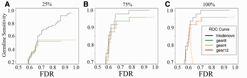
ROC curves of de novo germline SNV mutations called by TrioDeNovo and DeNovoGear in the 1000GP CEU trio data with different coverage. ROC curves were calculated on datasets with 25% (A), 75% (B) and 100% (C) of the original whole genome data. Black lines represent TrioDeNovo calls with flat prior odds. Green, orange and red lines represent DeNovoGear calls with specified mutation rates of 10⁻⁸ (default), 10⁻⁴ and 10⁻¹², respectively (color version of this figure is available at Bioinformatics online.)

False DNMs are often due to alignment artifacts, which are often uncaptured by current calling methods. We recently developed a machine-learning filtering tool, DNMFilter, which can effectively capture alignment artifacts and filter false positives (Liu et al., 2014). We investigated whether such a filtering scheme can be combined with TrioDeNovo to provide the research community a reliable pipeline that can further improve the accuracy of DNM calling. We re-calculated sensitivity and FDR of the candidates that passed the DNMFilter cutoff of 0.6. We observe significant improvements of germline mutation accuracy of TrioDeNovo calls on the full data (Fig. 4C), and the improvement is more pronounced when 75 and 25% of the data were used (Fig. 4A and B). For example, to achieve 80% sensitivity with 25% of the data, the FDR is 83% without filtering, and it is reduced to 63.6% when DNMFilter was used (Fig. 4A), indicating the effectiveness of DNMFilter in capturing false positives. For somatic mutations, we observed the same overall patterns of improvements after application of DNMFilter, although the effectiveness is not as dramatic as for germline mutations (Supplementary Fig. S4), probably due to unusual characteristics of cell line somatic mutations.

Fig. 4.

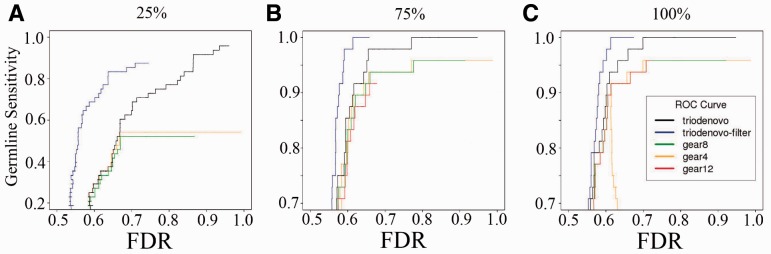
ROC curves of de novo germline SNV mutations called by TrioDeNovo and DeNovoGear in the 1000G CEU trio filtered using DNMfilter. Blue lines represent the ROC curves of the TrioDeNovo calls after applying DNMFilter and other lines are the same as those in Figure 3 (color version of this figure is available at Bioinformatics online.)

4 Discussion

Sequencing trios with sporadic-affected offspring has enabled the demystification of certain rare diseases and identification of genes implicated in complex disorders. Such a strategy will continue to be employed to decipher the genetic basis of disease. In this study, we developed an efficient and flexible framework to facilitate the DNM calling in parents-proband trios. The key advantage of our new method is the decoupling of mutation rates from evaluation of the data and the flexibility of adjusting the prior mutation odds post-hoc irrelevant of the data. This feature is important since DNM rates vary widely across the genome, and different classes of mutations exhibit varying mutation patterns. For example, the mutation rate for CpG dinucleotides is 9.5-fold that of non-CpG bases (Campbell et al., 2012). It is evident that mutation rates depend on multiple factors in a complex fashion, and it is not clear how contributing factors act together to influence the underlying mutations rate. With more families being sequenced, knowledge of DNMs is being accumulated quickly so that genome-wide mutation patterns can be soon accurately assessed. With such knowledge of prior mutation rates, TrioDeNovo is expected to further facilitate the DNM calling for the research community. Users have flexibility of adjusting the ranking of candidate mutations based on their knowledge without re-calling the mutations. Even in its simplest form with flat prior odds, TrioDeNovo outperformed existing state-of-the-art methods. Although tested on whole genome sequencing, TrioDeNovo can be equally applicable to exome sequencing data. The information used in TrioDeNovo is the pileup of bases aligned to each of the positions in the genome, and the alignment of reads from whole genome and exome data has similar accuracy in that regard.

The quality scores from TrioDeNovo have a natural interpretability as a BF. For example, a DQ value of 9 indicates that the likelihood of mutation is 10⁹ times of that without mutation. If a prior mutation rate of 10⁻⁹ is assumed, the candidate shows reasonable evidence of being a true mutation, and for a mutation rate of 10⁻⁸, a 10-fold increase of likelihood is given to this candidate. Such an interpretation is intuitive, and the adjustment does not require re-calling. On the other hand, the posteriors from other methods, e.g. DeNovoGear and Polymutt, do not have such a natural interpretation. These algorithms calculate the likelihood of data by a mixture of distributions of both Mendelian transmissions (M₀) and DNMs (M₁) in the same model. The relative contribution of M₁ and M₀ in the model is determined by the mutation rate, making the model sensitive to the pre-specified prior. Moreover, the relative ranking of candidates of DeNovoGear calls could change for the same data when different priors were used, which is rather undesirable.

Tools specialized for variant calling continue to improve the GL calculation and it is standard that these tools output GLs in the VCF file. By taking VCF files as input, TrioDeNovo can continuously benefit from these improvements without changing the interface. Furthermore, TrioDeNovo can be applied to VCF files generated by different tools, e.g. GATK, Samtools, FreeBayes and others, so that a consensus call set can be generated. The consensus approach has been shown to generate high-quality calls (Nielsen et al., 2011), and TrioDeNovo enables the consensus calling by integrating GLs calculated from various tools through the standard VCF input. In addition, TrioDeNovo runs very fast due to its efficient implementation so that consensus calling can be carried out efficiently.

TrioDeNovo calculates the mutation evidence based on the GLs at individual positions. Alignment artifacts are usually not well captured in the GLs and therefore can introduce false positive calls. Although VCF files contain some information about alignments, the information is insufficient to effectively distinguish real and artifactual mutations. We previously developed a machine-learning approach, DNMFilter, for filtering by incorporating rich features in bam files. DNMFilter was initially trained using exome sequencing data and showed improved accuracy on the 1000GP whole genome sequencing. We will further exploiting a training set of whole genome DNMs when more data are available. We hope that TrioDeNovo equipped with DNMFilter provides a powerful tool for mutation detection in trios for both targeted and whole genome sequencing. The C++ source code implementing TrioDeNovo and related resources are available on the authors’ website (https://medschool.vanderbilt.edu/cgg).

Funding

This work was partially supported by National Institutes of Health [grant 1R01HG006857 to Q.W., and B.L.] and [1R01HG007358 to W.C.].

Conflict of Interest: none declared.

References

- Campbell C.D., et al. (2012) Estimating the human mutation rate using autozygosity in a founder population. Nat. Genet. , 44, 1277–1281. [DOI] [PMC free article] [PubMed] [Google Scholar]
- Conrad D.F., et al. (2011) Variation in genome-wide mutation rates within and between human families. Nat. Genet. , 43, 712–714. [DOI] [PMC free article] [PubMed] [Google Scholar]
- Danecek P., et al. (2011) The variant call format and VCFtools. Bioinformatics , 27, 2156–2158. [DOI] [PMC free article] [PubMed] [Google Scholar]
- DePristo M.A., et al. (2011) A framework for variation discovery and genotyping using next-generation DNA sequencing data. Nat. Genet. , 43, 491–498. [DOI] [PMC free article] [PubMed] [Google Scholar]
- Fromer M., et al. (2014) De novo mutations in schizophrenia implicate synaptic networks. Nature , 506, 179–184. [DOI] [PMC free article] [PubMed] [Google Scholar]
- Gauthier J., et al. (2010) De novo mutations in the gene encoding the synaptic scaffolding protein SHANK3 in patients ascertained for schizophrenia. Proc. Natl Acad. Sci. USA , 107, 7863–7868. [DOI] [PMC free article] [PubMed] [Google Scholar]
- Gregor A., et al. (2013) De novo mutations in the genome organizer CTCF cause intellectual disability. Am. J. Hum. Genet. , 93, 124–131. [DOI] [PMC free article] [PubMed] [Google Scholar]
- Gulsuner S., et al. (2013) Spatial and temporal mapping of de novo mutations in schizophrenia to a fetal prefrontal cortical network. Cell , 154, 518–529. [DOI] [PMC free article] [PubMed] [Google Scholar]
- Hehir-Kwa J.Y., et al. (2011) De novo copy number variants associated with intellectual disability have a paternal origin and age bias. J. Med. Genet. , 48, 776–778. [DOI] [PubMed] [Google Scholar]
- Iossifov I., et al. (2012) De novo gene disruptions in children on the autistic spectrum. Neuron , 74, 285–299. [DOI] [PMC free article] [PubMed] [Google Scholar]
- Levy D., et al. (2011) Rare de novo and transmitted copy-number variation in autistic spectrum disorders. Neuron , 70, 886–897. [DOI] [PubMed] [Google Scholar]
- Li H., Durbin R. (2009) Fast and accurate short read alignment with Burrows–Wheeler transform. Bioinformatics , 25, 1754–1760. [DOI] [PMC free article] [PubMed] [Google Scholar]
- Li H., et al. (2009) The sequence alignment/map format and SAMtools. Bioinformatics , 25, 2078–2079. [DOI] [PMC free article] [PubMed] [Google Scholar]
- Li B., et al. (2012) A likelihood-based framework for variant calling and de novo mutation detection in families. PLoS Genet. , 8, e1002944. [DOI] [PMC free article] [PubMed] [Google Scholar]
- Liu Y., et al. (2014) A gradient-boosting approach for filtering de novo mutations in parent-offspring trios. Bioinformatics , 30, 1830–1836. [DOI] [PMC free article] [PubMed] [Google Scholar]
- Maiti S., et al. (2011) Ontogenetic de novo copy number variations (CNVs) as a source of genetic individuality: studies on two families with MZD twins for schizophrenia. PLoS ONE , 6, e17125. [DOI] [PMC free article] [PubMed] [Google Scholar]
- McKenna A., et al. (2010) The Genome Analysis Toolkit: a MapReduce framework for analyzing next-generation DNA sequencing data. Genome Res. , 20, 1297–1303. [DOI] [PMC free article] [PubMed] [Google Scholar]
- Neale B.M., et al. (2012) Patterns and rates of exonic de novo mutations in autism spectrum disorders. Nature , 485, 242–245. [DOI] [PMC free article] [PubMed] [Google Scholar]
- Nielsen R., et al. (2011) Genotype and SNP calling from next-generation sequencing data. Nat. Rev. Genet. , 12, 443–451. [DOI] [PMC free article] [PubMed] [Google Scholar]
- O'Roak B.J., et al. (2011) Exome sequencing in sporadic autism spectrum disorders identifies severe de novo mutations. Nat. Genet. , 43, 585–589. [DOI] [PMC free article] [PubMed] [Google Scholar]
- O'Roak B.J., et al. (2012) Sporadic autism exomes reveal a highly interconnected protein network of de novo mutations. Nature , 485, 246–250. [DOI] [PMC free article] [PubMed] [Google Scholar]
- Ramu A., et al. (2013) DeNovoGear: de novo indel and point mutation discovery and phasing. Nat. Methods , 10, 985–987. [DOI] [PMC free article] [PubMed] [Google Scholar]
- Ronemus M., et al. (2014) The role of de novo mutations in the genetics of autism spectrum disorders. Nat. Rev. Genet. , 15, 133–141. [DOI] [PubMed] [Google Scholar]
- Sanders S.J., et al. (2012) De novo mutations revealed by whole-exome sequencing are strongly associated with autism. Nature , 485, 237–241. [DOI] [PMC free article] [PubMed] [Google Scholar]
- Sebat J., et al. (2007) Strong association of de novo copy number mutations with autism. Science , 316, 445–449. [DOI] [PMC free article] [PubMed] [Google Scholar]
- Vissers L.E., et al. (2010) A de novo paradigm for mental retardation. Nat. Genet. , 42, 1109–1112. [DOI] [PubMed] [Google Scholar]
Associated Data
This section collects any data citations, data availability statements, or supplementary materials included in this article.