In silico Estimates of Tissue Components in Surgical Samples Based on Expression Profiling Data

Abstract

Tissue samples from many diseases have been used for gene expression profiling studies, but these samples often vary widely in the cell types they contain. Such variation could confound efforts to correlate expression with clinical parameters. In principle, the proportion of each major tissue component can be estimated from the profiling data and used to triage samples before studying correlations with disease parameters. Four large gene expression microarray data sets from prostate cancer, whose tissue components were estimated by pathologists, were used to test the performance of multivariate linear regression models for in silico prediction of major tissue components. Ten-fold cross-validation within each data set yielded average differences between the pathologists' predictions and the in silico predictions of 8% to 14% for the tumor component and 13% to 17% for the stroma component. Across independent data sets that used similar platforms and fresh frozen samples, the average differences were 11% to 12% for tumor and 12% to 17% for stroma. When the models were applied to 219 arrays of “tumor-enriched” samples in the literature, almost one quarter were predicted to have 30% or less tumor cells. Furthermore, there was a 10.5% difference in the average predicted tumor content between 37 recurrent and 42 nonrecurrent cancer patients. As a result, genes that correlated with tissue percentage generally also correlated with recurrence. If such a correlation is not desired, then some samples might be removed to rebalance the data set or tissue percentages might be incorporated into the prediction algorithm. A web service, “CellPred,” has been designed for the in silico prediction of sample tissue components based on expression data.

Introduction

Microarray expression profiles from dissected cancer samples have been used with clinical data to identify genes associated with disease status (for examples, see refs. 1–3). Any unrecognized differences in tissue components among samples will add noise to the measurement of gene expression, making relevant differences between two clinically distinct groups more difficult to detect. The main approach that has been used to try to reduce this variability is laser capture microdissection (LCM; refs. 4, 5). However, most available data were not acquired in this manner. As we will show, the public sets of expression data for bulk prostate cancer samples contain large differences in tissue components and some data sets have systematic differences in tissue composition correlating with clinical parameters. Such factors limit what can be extracted with confidence from these data sets. Taking into account tissue composition may improve the chances of identifying genuine biomarkers.

Various methods have been used to estimate tissue percentage in tissues (2, 6–8). In an earlier study, we examined the cell composition of a series of fresh surgical specimens from prostate cancer patients by expression analysis using 88 Affymetrix U95Av2 GeneChips (2). The cell compositions were estimated by a panel of four pathologists. Expression analysis was carried out on RNA prepared from the same samples. To identify tissue-specific genes, we used a linear combination model in which the expression level of a gene is the sum of contributions from each of the cell types where each contribution was the product of the percent of the cell type present and the characteristic expression coefficient for that cell type. The average percentage from the four pathologists was used. Because the estimated percent composition values and the total gene expression values are known, the expression coefficients for each cell type may be found for a series of samples by linear regression analysis. Of the 12,626 genes represented on the arrays, 1,098 were principally expressed by tumor cells and 683 were predominately expressed by stroma cells, with a smaller proportion of genes being predominately expressed by benign prostatic hyperplasia (BPH) epithelial cells and by the epithelial cells of dilated cystic glands. The gene specificity of the expression coefficients was validated by laser capture microdissected tumor cells, stroma cells, and epithelial cells of BPH samples and assessment of gene expression by quantitative PCR (2).

In this study, we perform the reverse calculation, using the above linear models to predict the tissue component of the samples based on the microarray data. The model seeks out those genes that are reflective of the tissue regardless of the clinical state of the samples. Thus, for example, the model will tend to exclude genes that correlate with tumor aggression or genes that change in reactive stroma. The prediction model is tested by 10-fold cross-validation within each data set and also by mutual prediction across independent data sets. In principle, estimates of the proportion of tissue components in each case could be used for triage or could be incorporated into prediction models, thereby reducing the effect of tissue proportions as a major source of variability among samples.

Materials and Methods

The tools presented here have been implemented in a web service called CellPred (Cell Predictor; ref. 15). Readers are referred to this web site for models that include complex variables.

Prostate cancer microarray data sets

Four publicly available prostate cancer data (data set 1 through 4) with pathologists' estimated tissue component information were included in this study (Table 1). For all these data sets, four major tissue components (tumor cells, stroma cells, epithelial cells of BPH, and epithelial cells of dilated cystic glands) were determined from sections immediately before and after the sections that were pooled for RNA preparation. The tissue component distributions for the four data sets are shown in Table 1.

Table 1. Prostate cancer microarray data sets with known tissue component information.

	Data set 1	Data set 2	Data set 3	Data set 4
Microarray platform	U133A	U133Plus2.0	U95Av2	Illumina DASL arrays
Sample type	Fresh frozen	Fresh frozen	Fresh frozen	FFPE
Arrays	136	149	88	114
Sample source
Prostatectomy	132	110	88	114
Autopsy*	4	13
LCM†		16‡
Prostate biopsy		10
Data source	GSE8218	GSE17951	GSE1431	Ref. 13
Reference	This work	This work	Ref. 2	Ref. 13
Probes or probe sets	22283	54675	12626	511
No. of pathologists	4	1	4	1
Tumor (%)
Maximum	80	100	80	90
Mean	20	26	17	24
Minimum	0	0	0	0
Stroma (%)
Maximum	100	100	100	100
Mean	61	63	59	54
Minimum	4	0	4	0
Epithelium from BPH (%)
Maximum	50	53	55	60
Mean	11	6	12	14
Minimum	0	0	0	0
Atrophic gland (%)
Maximum	20	49	32	50
Mean	6	4	7	7
Minimum	0	0	0	0

^*Autopsy prostate samples from normal subjects.

^†Laser capture microdissected samples.

^‡Twelve tumor samples and four stroma samples.

We also collected four publicly available microarray data sets (data set 5 through 8; refs. 10–13; Table 2) with a total of 238 arrays that were generated from 219 tumor-enriched and 19 nontumor parts of prostate tissue. Data set 5 consists of 79 samples in two groups (37 samples from patients where the cancer recurred and 42 samples from patients where recurrence did not occur within a few years after surgery). The samples used in these four data sets do not have associated tissue percentage estimates.

Table 2. Prostate cancer microarray data sets without known tissue component information.

	Data set 5	Data set 6	Data set 7	Data set 8
Array platform	U133A	U133A	U133Plus2.0	U133Plus2.0
Arrays	79	57	19	83
Sample type	Fresh frozen	Fresh frozen	Fresh frozen	Fresh frozen
Tumor-enriched samples	79	44	13	83
Stroma samples	0	13	6	0
Data source	Ref. 19	Ref. 20	GSE3325	GSE2109
Reference	Ref. 11	Ref. 10	Ref. 12	ExpO

Abbreviation: ExpO, Expression Project for Oncology.

Selection of genes for model training

Subsets of genes were selected to train prediction models within data set 1, 2, 3, or 4. The genes were ranked by their F-statistic, a measure of their fit in a multiple linear regression model as described below. Then different numbers of the highest ranked genes were compared for their performance on the training and test sets.

Multiple linear regression model

See “Main Model Equation.”

Cross-validation within data sets

Ten-fold cross-validation was used to estimate the prediction error rates for each data set. The prediction error rate for each individual sample is defined as the difference between the in silico predicted tissue percentages and the pathologists' estimates. The prediction error rate for an entire data set is the average of the absolute difference of these errors. Briefly, 10% of the samples were randomly selected as the test set using a permutation and the remaining 90% of the samples were used as a training set. Prediction models are constructed using the training sets with a predefined number of genes selected with the strategy mentioned above. The prediction is then applied to the test set. The sample selection and prediction step are repeated 10 times using different test samples each time until all the samples are used as test samples only once. This whole procedure is repeated five times using different sets of 10% of the data in each iteration.

Validation between data sets

Mutual predictions were performed among data sets 1, 2, 3, and 4 to assess the applicability of prediction models across different data sets. Because the microarray platforms differ among the four data sets, quantile normalization was applied to preprocess the microarray data (14) with one modification. The quantile normalization method was applied on the test data set with the entire training data set as the reference. This change means that the training set that is used to build prediction models are not recalculated and the prediction models will likely stay the same.

The mapping of probe sets from different Affymetrix platforms used the comparison files at the Affymetrix website (9). Probe sets in Affymetrix U133A array are subset of those in Affymetrix U133Plus2.0 array; thus, the performance of these two platforms are likely to be very similar for genes they have in common. The Illumina DASL platform used in data set 4 provided only gene symbols as the probe annotation, which was used to map to Affymetrix platforms. The numbers of genes mapped among different platforms are shown in Supplementary Table S1.

Prediction on data sets that do not have pathologists' estimates of tissue proportions

Data sets 5, 6, 7, and 8 do not have pathologists' estimates of tissue composition (Table 2). Data sets 1, 5, and 6 were generated from Affymetrix U133A arrays. Thus, the prediction models constructed with data set 1 were used to predict tissue components of samples used in data sets 5 and 6. Likewise, data sets 2, 7, and 8 were generated with Affymetrix U133Plus2.0 arrays; thus, prediction models constructed with data set 2 were used to predict tissue components of samples used in data sets 7 and 8. The modified quantile normalization method described above was used for preprocessing the test data sets.

Results and Discussion

Comparison of in silico predictions and pathologists' estimates within the same data set

Four sets of microarray expression data for which tissue percentages had been determined by pathologists (Table 1) were used to develop in silico models to predict tissue percentages. First, the effectiveness of the models was determined by measuring the discrepancies between in silico predictions and pathologists' estimates within the first four data sets using 10-fold cross-validation. To assess the best number of genes to be used in the prediction model, we constructed prediction models using different numbers of genes (i.e., 5, 10, 20, 50, 100, and 250). Genes were ranked by the F-statistic, a measure of their fit in the multiple linear regression model. The mean absolute differences between the values predicted in silico and the values estimated by pathologists as well as the correlation coefficients are shown in Table 3.

Table 3. Tumor and stroma tissue estimates using 10-fold cross-validation: in silico prediction compared with estimates by pathologists.

	Data set 1	Data set 2	Data set 3	Data set 4
5-gene model
Tumor cells	10.1/0.78	22.9/0.41 1	6.5/0.48	16.1/0.64
Stroma	20.8/0.51	28.4/0.38 3	1.9/0.16	21.5/0.5
10-gene model
Tumor cells	8.5/0.83	12.6/0.84	11.6/0.7	13.7/0.71
Stroma	18/0.57	19.6/0.61 2	1.7/0.52	17.8/0.62
20-gene model
Tumor cells	8.2/0.85	11.8/0.86 1	0.5/0.74	14.7/0.63
Stroma	15.9/0.64	16.6/0.72	18.6/0.5	18.6/0.6
50-gene model
Tumor cells	8.4/0.86	11.7/0.85 1	0.9/0.72	13.9/0.69
Stroma	13.3/0.72	14.3/0.78 1	8.3/0.55	16.9/0.66
100-gene model
Tumor cells	8/0.87	10.6/0.87 1	0.6/0.75	12.7/0.7
Stroma	12.9/0.74	13.5/0.79 1	7.1/0.56	15.6/0.7
250-gene model
Tumor cells	8.1/0.87	9.5/0.9 1	1.4/0.72	12.5/0.73
Stroma	12.8/0.73	12.5/0.82 1	7.3/0.57	15.4/0.72

NOTE: Data are percent discrepancy/correlation coefficient.

Figure 1 plots the mean differences versus the number of genes used in the prediction model. The in silico estimates reach maximum predictive power for tumor components with as few as 10 genes and for stroma components with about 50 genes. The in silico estimate based on using the 250-gene model is plotted against estimates by pathologists for tumor and stroma in these four data sets in Supplementary Fig. S1.

Figure 1.

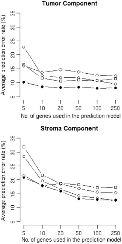
In silico tissue component prediction discrepancies compared with pathologists' estimates using 10-fold cross-validation. ●, data set 1; ○, data set 2; □, data set 3; ◊, data set 4. X axis, number of genes used in the prediction model. Y axis, average prediction error rates. A, prediction error rates for tumor components. B, prediction error rates for stroma components.

Among the four data sets, data set 1 has the most similar in silico prediction to the estimate made by pathologists, with an 8% average discrepancy rate for tumor and a 16% average discrepancy rate for stroma using the 250-gene model. The better performance of data set 1 may be explained by (a) this data set having estimates of tissue components from four pathologists, which is likely to be more accurate than estimates by one pathologist; (b) the use of fresh frozen tissues, which produce intact RNA for profiling; and (c) a relatively larger sample size. Data set 4 has the least accurate prediction, which may be ascribed to (a) the data set being generated from degraded total RNA samples from the formalin-fixed paraffin-embedded (FFPE) blocks and (b) far fewer genes being examined on the Illumina DASL array platform than any of the other array platforms: 511 probes versus 12,626 or more probe sets for the other data sets.

The predictions for tumor components are slightly more consistent than those for stroma. This may be partly explained by the fact that prostate stroma is a mixture of fibroblast cells, smooth muscle cells, blood vessels, etc.

Data set 2 contains 12 laser capture microdissected tumor samples; the average in silico predicted tumor component for these samples is 91%. Assuming these samples really are all nearly pure tumor, then the error rate is 9% or less for these samples, which is close to the average error rates of all samples in data set 2.

We have explored the possibility of predicting two other prostate cell types, the epithelial cells of benign prostatic hyperplasia (BPH) and the epithelial cells of dilated cystic glands, by extending the current multivariate model. We found that the in silico prediction of the proportion of these two tissue components is much less accurate than the predictions for the tumor and stroma components, largely because their percentages are usually small and pathologists differed widely in their estimates of these tissues. An extended prediction model that includes these tissues also does not improve the consistency of prediction of tumor and stroma components by the in silico model when compared with the estimates by pathologists (Supplementary Table S2). Taking the 250-gene model as example, we examined the error rates for the predictions made on different tissue types; the errors for BPH are much higher than those for the other two tissues, as shown in Supplementary Fig. S2. In general, for a tissue percentage to be useful for modeling in any disease, it is likely that estimates made by pathologists will need to be consistent and the range of percentages of each tissue type in the training set will need to be large before a reliable model for that tissue component can be built.

In the original study for data set 3, agreement analysis on the tissue components that were estimated by four pathologists was assessed as interobserver Pearson correlation coefficients. The average coefficients for tumor and stroma were 0.92 and 0.77 (2). This is better than the correlation coefficients between the in silico predictions and the pathologists' estimates for the same data set, which is 0.72 for the tumor component and 0.57 for stroma component (Table 3). However, the pathologists all reviewed the same section, whereas the tissue components of the adjacent samples that were processed for the array assay may differ. Certainly, some of the errors in the comparison between the pathologists' estimates and the in silico estimates can be attributed to variation between pathologists, and some of the errors can be attributed to the use of adjacent but nonidentical samples for arrays. Together, these factors indicate that in silico estimates may have substantially lower noise than that reported here.

One indication that the prediction model may be optimized to the limits of the data available is the fact that the discrepancy between in silico predicted tissue components of the test sets are generally within 1% of the predictions made on the training set. For example, the numbers for the 250-gene model are, for data set 1 (training/test): tumor, 7.6%/8.1%; stroma, 11.7%/12.8%; for data set 2 (training/test): tumor, 8.4%/9.5%; stroma, 11.5%/12.5%; for data set 3 (training/test): tumor, 10.3%/11.4%; stroma, 15.2%/17.3%; and for data set 4 (training/test): tumor, 11.9%/12.5%; stroma, 14.7%/15.4%. Data for models built using different numbers of genes are also very consistent (not shown).

Comparison between in silico predictions across data sets and pathologists' estimates

All four data sets that had cell composition estimates by pathologists (data sets 1, 2, 3, and 4) were compared with each other using a variety of tools. In Supplementary Table S3, each pair of data sets is compared using correlation coefficients among all genes (3A) and among each set of 250-gene models (3B) and the concordance in direction for each 250-gene model (3C). All of these measures showed strong and encouraging similarities among the data sets. For example, permutation analysis indicates that the concordance had a random probability of P < 10⁻⁸ for even the worst pairs of training and test data sets. Discrepancies for predictions made using 250-gene models across different data sets are shown in Table 4. In general, the in silico predictions across different data sets are less similar to the estimates by pathologists than the in silico predictions made within the same data set (Table 3). However, the discrepancy in predictions across data sets is similar to the discrepancy within data sets when the array platforms are very similar (Affymetrix U133A and U133Plus2.0) and sample types are the same (i.e., fresh frozen sample). For example, compare the average discrepancies for tumor within data sets 1 and 2 in Table 3 (8.1% and 8.0%) versus the discrepancies for each data set across these two data sets in Table 4 (11.0% and 11.6%). When microarray platforms or sample types differ (e.g., between fresh frozen and FFPE), the cross-data set prediction error rates increase and vary largely from 12.1% to 28.6% for tumor and from 14.7% to 38.2% for stroma, depending on the comparison. The mutual prediction results indicate the feasibility of tissue component predictions across data sets when array platform and sample type are the same. For other cases, where the platform or tissue quality is different, prediction of tissue percentages is also possible but has a significantly increased error.

Table 4. Tumor and stroma tissue estimates across data sets: in silico prediction compared with estimates by pathologists.

Test set/training set	Data set 1	Data set 2	Data set 3	Data set 4
Data set 1	NA	11.6/11.8 (0.82/0.73)	23.7/27 (0.86/0.74)	13.3/18.8 (0.82/0.75)
Data set 2	11/16.7 (0.89/0.76)	NA	22.1/38.2 (0.84/0.63)	28.6/25.8 (0.79/0.72)
Data set 3	14.5/15.1 (0.76/0.64	13.7/22.3 (0.75/0.59)	NA	17.4/14.7 (0.71/0.59)
Data set 4	12.1/24.5 (0.76/0.62)	12.7/23.7 (0.73/0.62)	12.8/19.9 (0.72/0.61)	NA

NOTE: Data are percent discrepancies for tumor/stroma (correlation coefficient for tumor/stroma). In silico predictions used 250-gene models.

In silico prediction of tissue components of samples in publicly available prostate data sets

The in silico predicted tumor and stroma components of 238 samples used in data sets 5, 6, 7, and 8 are documented in Supplementary Table S4. Of 238 samples, 219 were prepared as “tumor-enriched” prostate tissue (10–12). However, the in silico models predicted a wide range, from 0% to 87% tumor cells. Indeed, 50 (22.8%) samples were predicted to have less than or equal to 30% tumor cells (Fig. 2A). These 50 samples with low amounts of predicted tumor appeared in data set 5 [5 of 79 tumor samples (6.3%)], data set 6 [7 of 44 tumor samples (15.9%)], data set 7 [2 of 13 tumor samples (15.4%)], and data set 8 [30 of 83 tumor samples (36.1%)], suggesting that a large variation of tumor enrichment occurred in all four independent data sets.

Figure 2.

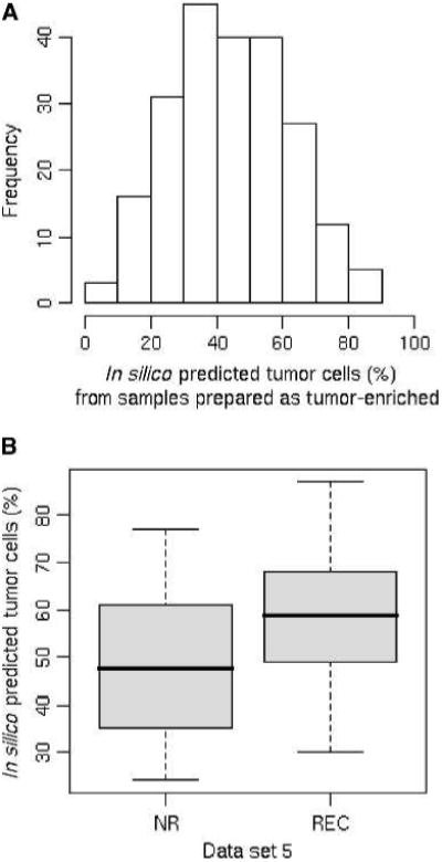
Tissue component predications on publicly available data sets. A, histogram of the in silico predicted tumor components of 219 arrays that were generated from samples prepared as tumor-enriched prostate cancer samples. X axis, in silico predicted tumor cell percentages. Y axis, frequency of samples. B, box plot shows the differences in tumor tissue components between the nonrecurrence and the recurrence groups of prostate cancer samples in data set 5. X axis, sample groups; NR, nonrecurrence group; REC, recurrence group. Y axis, tumor cell percentages.

Data set 5 includes information about recurrence of cancer after prostatectomy (11). We noticed that the average tumor tissue component predicted for the recurrence group (58.5%) is about 10% higher than that for the nonrecurrence group (48.0%), as shown in Fig. 2B. Unless recognized and taken into account, this skew has the potential to provide false data about recurrence. For example, tumor-specific genes might be significantly different in univariate analysis of the recurrent versus nonrecurrent cases simply because such genes are naturally enriched in samples with more tumor cells.

To further illustrate this effect, the percentage of tumor predicted on data set 5 using the data set 1 in silico model was plotted as the X axis in a heat map, with the nonrecurrence and recurrence groups plotted separately (Supplementary Fig. S3). The Y axis consists of the expression levels in data set 5 of the top 100 (50 upregulated and 50 downregulated) significantly differentially expressed genes between tumor and normal tissues identified in a third independent data set (data set 6). The gradient effects from left to right on the two groups (nonrecurrence and recurrence groups) of samples from data set 5 show that the expression levels of tissue-specific genes strongly correlate with the in silico predicted tumor content. Moreover, samples in the recurrence group show relatively higher expression level in upregulated genes and lower expression level in downregulated genes (Supplementary Fig. S3B), which indicates that the varying tumor components between the two groups may cause bias if the two groups were compared directly without corrections.

Software for prostate cancer tissue prediction

A web service, CellPred, has been developed to facilitate the prediction of tissue components of any type of tissue samples. The program accepts uploads of Affymetrix Cel files or any other type of expression data, such as relative expression levels derived from high-throughput expression sequence tags, if these data are condensed into a file equivalent to an intensity file. The program requires that there be a training set of expression data associated with tissue component information estimated by pathologists. The model built on the training set can then be applied to any test set to predict the tissue components of each sample in the test set. The user can build a model based on two or more tissues. The user can also include other variables to encompass any suspected systematic bias in the data, such as batch information or hospital of origin. However, it should be noted that although each additional variable will improve the fit in the training set, additional variables may not increase accuracy of prediction when the training data set is not sufficient to decompose the contributions of these variables.

To construct the prediction models, we adopted a 10-fold permutation strategy (see Materials and Methods). Users have the option to choose the number of top performing genes in the training set for constructing the model (e.g., 5, 10, 20, 50, 100, or 250 genes). The expression properties of these top genes are then used to predict the tissue percentages in the test samples. Other details about the program can be found in the online help document.

As an example, data have already been uploaded to allow prediction models constructed on data sets 1, 2, 3, and 4 (Affymetrix U133A, U133Plus2.0, U95Av2 array, and Illumina DASL array) to be used for making predictions for a user-supplied data set of prostate samples. We used 5-, 10-, 20-, 50-, 100-, and 250-gene models for each data set. These lists were used to construct prediction models that were integrated into the CellPred program. Thus, users that have access to a new set of expression data for prostate cancer do not need a training set to estimate the tissue percentages in their samples.

The lists of genes used in prediction of tissue percentages in these models are substantially different between test data sets, even when these data sets share the same platform (Supplementary Table S5). This lack of overlap is not due to a lack of consistency among data sets. On the contrary, the reason for this phenomenon is that the different cell types (tumor and stroma) differ in the expression of thousands of genes, all of which have some power to estimate tissue percentages. For example, of the top 50 genes in data set 2 used for tissue prediction, 33 (70%) are found in the top 500 (2%) of data set 1, and in the opposite comparison the number is 35 (66%). Thus, the genes identified as the most useful for tissue percentage estimation in one data set are generally also highly correlated with tissue percentages in other data sets.

CellPred is integrated into our microarray data analysis suite (15). CellPred was developed on a LAMP system (a GNU/Linux server with Apache, MySQL and Python). The modules were written in python (16) whereas analysis functions were written in R language (17). CellPred and the R script for modeling/training/prediction are downloadable from our website (18).

Summary

In this study, we explored the feasibility of in silico prediction of tissue components of prostate samples using high-throughput expression data. We identified subsets of genes that predict stroma and tumor, excluding any genes that were responding to specific clinical differences between samples. These genes showed an excellent correlation between in silico predictions and estimates by pathologists within data sets. When estimates were made across data sets that used the same type of sample (e.g., fresh frozen samples) and similar platforms (e.g., Affymetrix U133A and U133Plus2.0 arrays), there was also a low discrepancy from estimates made by pathologists: ∼11% average discrepancy for tumor and 12% to 17% for stroma components across data sets. Applying these prediction models to data sets on the same platform and with the same type of sample (fresh frozen), we showed that in silico prediction could be a valuable step for quality control of expression data sets from samples that may contain multiple cell types. We observed a significant but possibly spurious correlation between the proportion of tumor in prostate cancer and recurrence of disease in one data set. If this correlation is not taken into account, it could lead to identification of tissue-specific genes as being associated with recurrence.

Overall, there is a good correlation between estimates made by pathologists and estimates made in silico; however, there are some samples that show a poor correlation (see Supplementary Fig. S1 for examples). This is not necessarily attributable to errors in the in silico estimates. The pathologists also differ among themselves in estimating samples, with a variation of more than 5% in their estimates, which is about half of the variability seen between the pathologist and the in silico estimates. Furthermore, the samples used for in silico estimates are adjacent but not identical to the samples assayed by pathologists. Some of the discrepancies between the pathologists' estimates and the in silico estimates are likely to be attributable to these factors, implying that in silico measurements are substantially more accurate than the estimates presented here. Indeed, one cannot rule out the possibility that estimates made in silico are superior to estimates made by pathologists.

The strategy of in silico prediction of tissue types in mixed samples might be extended to thousands of arrays and increasing numbers of high-throughput sequence tag data that have already been accumulated in the GEO database for solid tissue samples from a variety of diseases, not just cancer. Even supposedly pure LCM samples might benefit from such a screen. All that is needed are gene expression data for disease samples where a wide range of tissue composition estimates have been made by pathologists, then an in silico prediction model can be developed and applied to other data sets.

Major Findings.

Prediction of tissue proportions can expose large composition differences among surgical samples. Such knowledge will allow triage of samples before correlation with clinical data or could be incorporated into models before such correlations are performed. In principle, prediction of major tissue composition can be extended to any clinical samples once a training set that contains a range of known tissue compositions is available.

Quick Guide: Main Model Equation

$$g={\beta }_0+\sum _{j=1}^C{\beta }_j{p}_j+e$$

A multivariate linear regression model was used for predicting tissue components, where g is the expression value for a gene, p_j is the percentage of a given tissue component determined by the pathologists, and β_j is the expression coefficient associated with a given cell type. In this model, C is the number of tissue types under consideration. β_j estimates the relative expression level in cell type j compared with the overall signal level of all the other cell types that are represented by β₀. e is the random error.

Genes that best predict tissue percentage as independently estimated by pathologists are established in a training set. Then, g and β_j from each of these “predictive” genes are applied to the expression data in another data set to estimate the tissue percentage of each sample by solving for p_j using linear regression.

Major Assumptions of the Model

This model assumes that the observed gene expression intensity of a gene is the sum of the contributions from different types of cells and that this relationship remains similar between different clinical samples. Thus, the model assumes that when one of the two variables, p_s and βs, are given, then the other variable can be estimated using a linear regression model. The model also assumes there are some genes that are associated with tissue percentage, regardless of biological and technical variability. Such genes will be highly ranked in the training set. When a gene does not comply with these assumptions, such as a gene regulated between different clinical samples or regulated depending on its location relative to tumor (e.g., a gene that changes in reactive stroma), then the model will rank the gene low and it will be excluded from being used to predict tissue percentages in other data sets.

References

- 1.Sorlie T, Tibshirani R, Parker J, et al. Repeated observation of breast tumor subtypes in independent gene expression data sets. Proc Natl Acad Sci U S A. 2003;100:8418–23. doi: 10.1073/pnas.0932692100. [DOI] [PMC free article] [PubMed] [Google Scholar]
- 2.Stuart RO, Wachsman W, Berry CC, et al. In silico dissection of cell-type-associated patterns of gene expression in prostate cancer. Proc Natl Acad Sci U S A. 2004;101:615–20. doi: 10.1073/pnas.2536479100. [DOI] [PMC free article] [PubMed] [Google Scholar]
- 3.Wang Y, Klijn JG, Zhang Y, et al. Gene-expression profiles to predict distant metastasis of lymph-node-negative primary breast cancer. Lancet. 2005;365:671–9. doi: 10.1016/S0140-6736(05)17947-1. [DOI] [PubMed] [Google Scholar]
- 4.Paweletz CP, Liotta LA, Petricoin EF., III New technologies for biomarker analysis of prostate cancer progression: Laser capture microdissection and tissue proteomics. Urology. 2001;57:160–3. doi: 10.1016/s0090-4295(00)00964-x. [DOI] [PubMed] [Google Scholar]
- 5.Sgroi DC, Teng S, Robinson G, LeVangie R, Hudson JR, Jr, Elkahloun AG. In vivo gene expression profile analysis of human breast cancer progression. Cancer Res. 1999;59:5656–61. [PubMed] [Google Scholar]
- 6.Cleator SJ, Powles TJ, Dexter T, et al. The effect of the stromal component of breast tumours on prediction of clinical outcome using gene expression microarray analysis. Breast Cancer Res. 2006;8:R32. doi: 10.1186/bcr1506. [DOI] [PMC free article] [PubMed] [Google Scholar]
- 7.Wang M, Master SR, Chodosh LA. Computational expression deconvolution in a complex mammalian organ. BMC Bioinformatics. 2006;7:328. doi: 10.1186/1471-2105-7-328. [DOI] [PMC free article] [PubMed] [Google Scholar]
- 8.Clarke J, Seo P, Clarke B. Statistical expression deconvolution from mixed tissue samples. Bioinformatics. 26:1043–9. doi: 10.1093/bioinformatics/btq097. [DOI] [PMC free article] [PubMed] [Google Scholar]
- 9.Affymetrix web site [homepage on the Internet]. Downloadable files containing mapping information across different Affymetrix array plaforms are available after a free registration at: http://www.affymetrix.com
- 10.Liu P, Ramachandran S, Ali Seyed M, et al. Sex-determining region Y box 4 is a transforming oncogene in human prostate cancer cells. Cancer Res. 2006;66:4011–9. doi: 10.1158/0008-5472.CAN-05-3055. [DOI] [PubMed] [Google Scholar]
- 11.Stephenson AJ, Smith A, Kattan MW, et al. Integration of gene expression profiling and clinical variables to predict prostate carcinoma recurrence after radical prostatectomy. Cancer. 2005;104:290–8. doi: 10.1002/cncr.21157. [DOI] [PMC free article] [PubMed] [Google Scholar]
- 12.Varambally S, Yu J, Laxman B, et al. Integrative genomic and proteomic analysis of prostate cancer reveals signatures of metastatic progression. Cancer Cell. 2005;8:393–406. doi: 10.1016/j.ccr.2005.10.001. [DOI] [PubMed] [Google Scholar]
- 13.Bibikova M, Chudin E, Arsanjani A, et al. Expression signatures that correlated with Gleason score and relapse in prostate cancer. Genomics. 2007;89:666–72. doi: 10.1016/j.ygeno.2007.02.005. [DOI] [PubMed] [Google Scholar]
- 14.Bolstad BM, Irizarry RA, Astrand M, Speed TP. A comparison of normalization methods for high density oligonucleotide array data based on variance and bias. Bioinformatics. 2003;19:185–93. doi: 10.1093/bioinformatics/19.2.185. [DOI] [PubMed] [Google Scholar]
- 15.Xia XQ, McClelland M, Porwollik S, Song W, Cong X, Wang Y. WebArrayDB: cross-platform microarray data analysis and public data repository. Bioinformatics. 2009;25:2425–9. doi: 10.1093/bioinformatics/btp430. [DOI] [PMC free article] [PubMed] [Google Scholar]
- 16.Python Programming Language. [homepage on the Internet]. Open source download available at http://www.python.org.
- 17.The R Project for Statistical Computing. [homepage on the Internet]. Open source download available at http://www.r-project.org/
- 18.Web site of CellPred (http://www.webarray.org/cellpred/), Webarray, and WebarrayDB [homepage on the Internet]. Open source download available at http://www.webarray.org
- 19.Koziol JA, Feng AC, Jia Z, et al. The wisdom of the commons: ensemble tree classifiers for prostate cancer prognosis. Bioinformatics. 2009;25:54–60. doi: 10.1093/bioinformatics/btn354. [DOI] [PMC free article] [PubMed] [Google Scholar]
- 20.European Bioinformatic Institute website. Freely available data deposited at http://www.ebi.ac.uk/microarray-as/ae/browse.html?keywords=E-TABM-26.
Associated Data
This section collects any data citations, data availability statements, or supplementary materials included in this article.