

Abstract
The aim of this work was to quantitatively model cross‐sectional relationships between structural connectome disruptions caused by cerebral infarction and measures of clinical performance. Imaging biomarkers of 41 ischemic stroke patients (72.0 ± 12.0 years, 20 female) were related to their baseline performance in 18 cognitive, physical and daily life activity assessments. Individual estimates of structural connectivity disruption in gray matter regions were computed using the Change in Connectivity (ChaCo) score. ChaCo scores were utilized because they can be calculated using routinely collected clinical magnetic resonance imagings. Partial Least Squares Regression (PLSR) was used to predict various acute impairment and activity measures from ChaCo scores and patient demographics. Statistical methods of cross‐validation, bootstrapping and multiple comparisons correction were implemented to minimize over‐fitting and Type I errors. Multiple linear regression models based on lesion volume and lateralization information were constructed for comparison. All models based on connectivity disruption had lower Akaike Information Criterion and almost all had better goodness‐of‐fit values (R 2: 0.26–0.92) than models based on lesion characteristics (R 2: 0.06–0.50). Confidence intervals of PLSR coefficients identified brain regions important in predicting each clinical assessment. Appropriate mapping of eloquent functions, that is, language and motor, and replication of results across pathologies provided validation of this method. Models of complex functions provided new insights into brain‐behavior relationships. In addition to the potential applications in prognostication and rehabilitation development, this quantitative approach provides insight into the structural networks underlying complex functions like activities of daily living and cognition. Quantitative analysis of big data will be invaluable in understanding complex brain‐behavior relationships. Hum Brain Mapp 36:2147–2160, 2015. © 2015 Wiley Periodicals, Inc.
Keywords: connectome, biological markers, outcome assessment (health care), stroke, magnetic resonance imaging, infarction, cognition, linear models
INTRODUCTION
The relationship between human cognition, language, motor control and behavior and anatomical and physiological brain networks largely remains a mystery. Traditionally, clinical‐pathological lesion mapping studies have provided a way for researchers to explore brain regions subserving specific functions [Broca, 1861; Wernicke, 1874] and, at times, more complex behaviors [Milner, 1982; Posner et al., 1988]. Neuroimaging techniques, that is, diffusion and functional magnetic resonance imaging (MRI), enable an unprecedented investigation of human brain anatomy and function. Recent works have used these in vivo techniques in lesion‐mapping studies to enhance our understanding of eloquent cortical areas, such as those responsible for language and motor functions [Butler et al., 2014; Hope et al., 2013; Phan et al., 2010], general intelligence[Barbey et al., 2012; Gläscher et al., 2010] and neglect[Mort et al., 2003]. However, the anatomical substrates underlying performance in more general tasks, like basic activities of daily living and more complex behaviors that arise from distributed brain networks, are not as fully understood. Machine learning techniques applied to neuroscientific “big data” sets will be central to understanding these complex brain‐behavior relationships.
One such machine learning technique is the method of partial least squares regression (PLSR)[Wold, 1982]. PLSR has been applied in the field of neuroimaging in previous studies of brain‐behavior relationships, mostly in the analysis of functional MRI [Hay et al., 2002; Itier et al., 2004] [see Krishnan et al., 2011 for a review]. For example, one study [Phan et al., 2010] investigated the impact of infarct size and location on motor and language function at a voxel‐wise level using a logistic version of PLSR. This work and that of others [Kuceyeski et al., 2011; Menezes et al., 2007] have reinforced the well‐established notion that the location of tissue damage is a key factor determining the attendant functional deficit, that is, sign or symptom. Advanced neuroimaging techniques and quantitative methods, for example, voxel‐based morphometry [Ashburner and Friston, 2000] and voxel‐based lesion‐symptom mapping [Bates et al., 2003], can be used to map voxel‐wise parameters to behavior. However, it is not only a lesion's location in gray matter (GM) that is important since damage can also disrupt white matter (WM) tracts that connect GM regions. This disruption of the brain's structural connections, in turn, affects function [Johansen‐Berg et al., 2010; Puig et al., 2013] and possibly recovery [Crofts et al., 2011; van Hees et al., 2014]. Therefore, we hypothesized that models based on measures of the brain's structural connectome disruption due to a lesion's size and location will result in more accurate predictions of clinical assessments than a model based on lesion characteristics.
To test this hypothesis, we used the recently developed Network Modification (NeMo) Tool [Kuceyeski et al., 2013] in conjunction with PLSR to link patterns of disruption in the brain's structural connectome to measures of various cognitive, motor, language and daily living activities in a cohort of patients with ischemic stroke, similar to [Kuceyeski et al., in press]. The NeMo Tool quantifies the amount of connectivity disruption that a given cortical or subcortical region has incurred due to a given WM lesion using normal subjects' structural connectivity information. This tool is attractive because it uses MRI sequences routinely obtained in the clinical setting after acute stroke and it does not suffer from the limitations of tractography techniques applied in patient data with tissue abnormalities [Pagani et al., 2007; Wheeler‐Kingshott and Cercignani, 2009]. It also offers an easy way for radiologists to compute complex and physiologically relevant quantitative MRI‐based biomarkers of structural network disruption in a variety of diseases. In conjunction with reducing the dimensionality of the data via PLSR, other statistical methods like cross‐validation, bootstrapping, and strict multiple comparisons correction of confidence intervals for model parameter across the entire study are implemented to minimize the risk of over‐fitting and Type I errors often associated with models involving a large number of predictor variables.
SUBJECTS AND METHODS
Data
Ninety‐two subjects with acute stroke were admitted to the inpatient rehabilitation unit (IRU) at New York‐Presbyterian (NYP) Hospital/Weill Cornell Medical Center between July 2012 and November 2013 and provided consent for participation in this IRB‐approved study. Subjects were included if they had (1) ischemic stroke, (2) MRI scans acquired at NYP within 14 days of stroke, and (3) apparent hyperintensities on diffusion‐weighted images (DWI). Forty‐one subjects (age: 72.0 ± 12.0 years, 20 female) satisfied these inclusion criteria, see Supporting Information Table I for cohort characteristics. Average time from stroke onset to imaging was 2.3 ± 3.4 days and average time from stroke onset to clinical assessments (IRU admission) was 8.1 ± 9.9 days. T1 and DWI were collected on 1.5 Tesla (34 subjects) or 3.0 Tesla (7 subjects) GE Signa EXCITE scanners (GE Healthcare, Waukesha, WI). The DWIs (on both 1.5 and 3.0 T) were acquired axially via an echo‐planar imaging sequence, with b = 1,000 and 0 s/mm2 from 30 5‐mm thick slices and 128 × 128 matrix size, 1 mm in‐plane resolution, 240 mm field‐of‐view, repetition time/echo time/inversion time = 8,000 or 10,000/100/0 ms. T1 scans were acquired axially (repetition time/echo time/inversion time = 500/10/0 ms for 1.5 T and 1,700/21/725 for 3.0 T) with a 256 × 256 matrix over 30 5.0‐mm thick slices with 0.5 mm in‐plane resolution and 240 mm field‐of‐view. One subject did not have a T1 available; the T2 scan was used instead for postprocessing. The T2 was an axial sequence (repetition time/echo time/inversion time = 4,000/85/0 ms) with a 256 × 256 matrix over 30 5.0‐mm contiguous partitions.
The National Institutes of Health Stroke Scale (NIHSS) [Brott et al., 1989] was administered acutely on initial presentation to the hospital, and a battery of cognitive, functional, and motor assessments were performed after transfer to the IRU. These tests, which assessed general stroke severity as well as motor, language, cognitive, and overall neurological ability, included the Upper and Lower Extremity Motricity Indices (MI) [Collin and Wade, 1990], Functional Independence Measures (FIM) [Keith et al., 1987], Montreal Cognitive Assessment (MOCA) [Nasreddine et al., 2005], and Symbol Digits Modality Test (SDMT) [Smith, 1982] (see Table 1). As aphasia is an impairment related to injury in specific regions, we also included the Mississippi Aphasia Screening Test (MAST) [Nakase‐Thompson et al., 2005] as a partial validation for our methodology.
Table 1.
Summary of data and model results for each assessment [Color table can be viewed in the online issue, which is available at http://wileyonlinelibrary.com.]
| Test Name | No. sub. | Raw Scores (mean ± std) | LS w/lesion vol. R 2 (AIC) | LS w/vol. & L/R R 2 (AIC) | Fixed‐effects PLSR R 2 (AIC) | Bootstrap PLSR R 2 (mean ± std) | No. PLSR comp | Predictors with nonzero PLSR regression coefficients (negative in red, positive in blue) | PLSR components |
|---|---|---|---|---|---|---|---|---|---|
| NIH Stroke Scale (negated) | 39 | 7.8 ± 5.9 | 0.43 (−11.6) | 0.46 (−8.82) | 0.76 (−51.26) | 0.78 ± 0.05 | 2 | age, bilateral pre/postcentral, superior frontal and supramarginal gyri; left paracentral gyri, parietal and subcortical areas | First: Cerebellar vs. noncerebellar |
| Second: Left vs. right | |||||||||
| Left LE MI | 39 | 76.9 ± 33.3 | 0.12 (5.75) | 0.36 (−2.54) | 0.35 (−13.95) | 0.38 ± 0.13 | 1 | right thalamus and other subcortical regions, frontal and parietal areas including the rolandic operculum, supplemental motor area and post/paracentral gyri, left hemisphere | Left vs. right |
| Right LE MI | 39 | 83.4 ± 24.3 | 0.24 (−0.14) | 0.50 (−11.89) | 0.50 (−22.50) | 0.54 ± 0.14 | 2 | left supramarginal gyri, right thalamus and subcortical, other left motor areas large but NS | Left vs. right |
| MIU Left UE MI | 38 | 77.4 ± 36.4 | 0.18 (3.41) | 0.31 (0.90) | 0.27 (−8.98) | 0.33 ± 0.13 | 1 | vermis and right parietal, occipital and frontal regions, including the cingulate structures, superior parietal gyri, para/postcentral gyri, and supplementary motor area, right hemi. | Left vs. right |
| MIU Right UE MI | 38 | 80.8 ± 34.3 | 0.21 (1.94) | 0.31 (0.64) | 0.39 (−16.21) | 0.46 ± 0.14 | 1 | vermis and right cerebellum, left motor regions large but NS | Left vs. right |
| Total MAST | 34 | 90.9 ± 20.5 | 0.31 (−2.02) | 0.38 (−1.21) | 0.92 (−82.42) | 0.87 ± 0.16 | 2 | left hemisphere regions, including rolandic operculum, postcentral gyri, frontal inferior operculum, insula, Heschl's gyri and globus pallidus; right frontotemporal | First: right |
| FIM motor | 41 | 34.3 ± 15. | 0.20 (1.72) | 0.20 (5.70) | 0.34 (−14.15) | 0.37 ± 0.08 | 1 | right frontal and parietal, hippocampus and caudate nucleus, pre/para/postcentral gyri, SMA and left superior parietal regions | First: language‐related, left frontotemporal |
| Second: left frontal and right temporal | |||||||||
| FIM cognitive | 41 | 24.9 ± 8.0 | 0.21 (0.88) | 0.27 (2.08) | 0.68 (−42.93) | 0.69 ± 0.07 | 2 | bilateral frontal, left parietal and subcortical regions | First: right |
| FIM total | 41 | 59.7 ± 22.1 | 0.23 (−0.15) | 0.24 (3.68) | 0.44 (−20.87) | 0.45 ± 0.08 | 1 | similar to FIM moto | First: Cerebellar vs. Noncerebellar |
| Second: Right frontotemporal‐pareital | |||||||||
| SDMT # Correct | 33 | 19.5 ± 11.2 | 0.10 (52.68) | 0.15 (55.10) | 0.39 (33.63) | 0.47 ± 0.11 | 2 | right inferior occipital and calcarine areas | First: right hemisphere |
| SDMT # attempted | 33 | 20.7 ± 10.8 | Second: right occipital vs. other right hemispheric regions | ||||||
| MOCA Visuospatial‐executive | 36 | 2.8 ± 1.5 | 0.18 (3.63) | 0.30 (2.27) | 0.34 (−10.25) | 0.37 ± 0.09 | 2 | left superior and inferior parietal regions, angular gyri, putamen and globus pallidus | First: Cerebellar vs. noncerebellar, right |
| Second: left vs. right | |||||||||
| MOCA Naming | 35 | 2.5 ± 0.6 | 0.25 (0.61) | 0.33 (0.91) | 0.43 (−15.16) | 0.45 ± 0.13 | 2 | bilateral globus pallidus, left angular gyrus and right amygdala, right occipital regions | First: left frontal/subcortical and right occipital |
| Second: Left frontal/subcortical vs. left occipital/cerebellar | |||||||||
| MOCA Attention | 36 | 4.2 ± 1.6 | 0.09 (7.47) | 0.14 (9.38) | 0.26 (−8.31) | 0.31 ± 0.09 | 1 | right inferior and superior fronto‐temporal‐parietal regions | First: right inferior and superior frontotemporal‐parietal regions |
| MOCA Language | 36 | 1.8 ± 0.9 | 0.06 (8.61) | 0.08 (12.10) | 0.38 (−12.68) | 0.43 ± 0.10 | 2 | bilateral medial regions, including middle and anterior cingulate and superior medial frontal gyri | First: left frontal vs. left temporal‐occipital |
| Second: medial versus lateral | |||||||||
| MOCA Abstraction | 36 | 1.5 ± 0.6 | 0.10 (7.00) | 0.15 (9.34) | 0.56 (−24.59) | 0.60 ± 0.11 | 2 | right medial parietal and medial frontal areas | First: medial regions |
| Second: Left frontotemporal‐pareital | |||||||||
| MOCA Delayed Recall | 36 | 1.6 ± 1.6 | 0.08 (7.96) | 0.12 (10.20) | 0.50 (−20.63) | 0.52 ± 0.10 | 2 | right amygdala, globus pallidus, rectus gyrus and some orbito‐frontal regions, left medial frontal superior | First: Medial regions |
| Second: Left occipital, bilateral parahippocampal and hippocampal vs. right frontotemporal | |||||||||
| MOCA Orientation | 36 | 5.3 ± 1.0 | 0.20 (2.59) | 0.26 (4.22) | 0.55 (−21.77) | 0.55 ± 0.14 | 3 | left superior and inferior parietal areas, vermis | different areas in the left frontoparietal |
| MOCA Total | 35 | 20.1 ± 5.1 | 0.12 (6.22) | 0.19 (7.46) | 0.28 (−8.66) | 0.30 ± 0.09 | 1 | right frontal and temporal regions | First: right frontotemporal pareital |
The NeMo Tool
The NeMo Tool infers changes to the structural connectivity network that may result from a given WM lesion by superimposing the patient's lesion mask on a database of 73 normal control tractograms in a common space (Montreal Neurological Institute, or MNI space). WM alteration masks in this cohort were created and processed as in our previous study [Kuceyeski et al., in press]. Specifically, masks indicating acute stroke injury as identified by apparent DWI hyperintensities were hand drawn; this method was shown to have a Dice's inter‐rater similarity index of 0.70 ± 0.12 (IQR: 0.64–0.83)[Kuceyeski et al., 2014]. The stroke subjects' T1 scans were normalized to MNI space using linear followed by nonlinear normalization in SPM8[Friston et al., 2006], and these transformations were then applied to the DWI mask with nearest neighbor interpolation. The NeMo Tool then estimated the amount of connectivity abnormalities each region incurred via the Change in Connectivity (ChaCo) score, that is, the percent of streamlines connecting to a given GM region that pass through an area of infarct. Higher ChaCo scores correspond to a higher percent of estimated connectivity disruption experienced by a given region.
Partial Least Squares Regression and Bootstrapping
PLSR [Wold et al., 1984] was used to predict each of the various clinical assessments from the input variables, namely, subject age, gender, number of days between stroke, and clinical assessment and ChaCo scores for 93 brain regions. We used a popular 116‐region cortical and subcortical region atlas [Tzourio‐Mazoyer et al., 2002] and averaged ChaCo values in the left cerebellum, right cerebellum, and vermis for a total of 93 cortical and subcortical regions. PLSR is advantageous in situations where there exist many more input variables than available data points, as the data gets reduced to a parsimonious set of statistically relevant components. PLSR reduces the dimensionality of the input variables by combining them into new variables (components) that have maximum correlation with the outcome variable, followed by regression on the new variables. Each newly created component is independent of the others, making PLSR useful when input variables may be colinear. Each input variable's component coefficient can be interpreted as relative weight that determines the contribution of that input variable to the given component. It must be noted that the sign of the component coefficient is not important except for relative comparison as they are invariant to reflection (sign flipping). The final number of components for the final model was chosen via jackknife cross‐validation to minimize data over‐fitting, and stability of the model was assessed using bootstrapping [Krishnan et al., 2011]. Confidence intervals for the regression coefficients were calculated using the bias corrected and accelerated percentile method [Efron, 1987]. If it did not include zero after correcting for multiple comparisons using the Bonferroni method [Dunn, 1961], it was considered a significant predictor for that assessment (see Supporting Information for details).
Comparison to Models Based on Lesion Volume and Volume Plus Lateralization
We compared the PLSR model results to those of two different models: one based on only volume of the patient's infarct and the other based on volume as well as lateralization of the infarct. To do this, we created multiple linear regression models for each clinical assessment that were based on important subject characteristics (age, gender, and number of days between the stroke and assessment) in addition to (1) lesion volume (after log transformation for better scaling) and (2) log lesion volume and lateralization (left, right, bilateral). In the latter model, we added two binomial variables to represent the three categories of lateralization. As there were only 4 or 6 input variables for the lesion volume models, we chose to use standard multiple linear regression in favor of the PLSR approach. Noncategorical input and output variables were centered and standardized before performing the regressions. R 2 values measuring goodness‐of‐fit and Akaike Information Criterion (AIC) [Burnham and Anderson, 2002] measuring goodness‐of‐fit while considering complexity were compared between the two models. The AIC provides a way to relatively compare models that have different input variables; smaller values of AIC indicate the preferred model. All models and statistical tests were performed using relevant programs within MATLAB.
RESULTS
Among 41 study subjects, mean lesion size, as calculated after normalization to MNI space, was 22.4 ± 41.3 cm3. Eighteen subjects had lesions affecting mostly right hemispheric connections (>70% of total ChaCo score came from right regions), 20 had mostly left (>70% of total ChaCo score came from left regions) and 3 had bilateral connectivity implications. ChaCo scores varied widely across the population due to the diverse location of the infarcts (see Fig. 1A) and were more prominent in the hemisphere with the lesion. “Glassbrain” displays in Figure 1B are used to visualize mean ChaCo scores. Spheres are plotted at the center of the region they represent and colored based on classification (blue = frontal, magenta = parietal, red = temporal, cyan = subcortical, and yellow = cerebellar). Sphere size is proportional to that region's mean ChaCo score (larger = more connectivity disruption). In general, areas with highest ChaCo included the subcortical areas of the caudate, putamen, globus pallidus, amygdala, thalamus, and insula in addition to the right pre/post central gyri, left cerebellum and right frontal areas. Parietal and temporal regions were also affected but to a lesser degree. Mean ChaCo scores, represented as percents, along with standard deviations are given in Supporting Information Table II.
Figure 1.
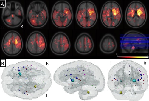
Summary of lesion location and structural connectome disruption. (Panel A) A voxelwise heat map of the lesions across the population. (Panel B) Mean ChaCo score for each region over the population of 41 subjects. Each sphere is located at the center of the corresponding GM region and its size is proportional to that region's mean ChaCo score (bigger = more network disruption). Colors indicate regional assignment to larger grouping (blue = frontal, magenta = parietal, red = temporal, cyan = subcortical and yellow = cerebellar).
Figure 2 and Table 1 summarize the goodness‐of‐fit (R 2) measures for the linear regression models based on lesion volume (black circles), lesion volume and lateralization (green circles), the fixed‐effects PLSR models based on ChaCo scores (cyan triangles) and the bootstrapped random effects PLSR models based on ChaCo scores for each clinical assessment (blue boxplots). The boxplots visualize the median (red line), interquartile range (blue box), range of the most extreme points not considered outliers (black whiskers), and outliers (red points). Fixed‐effects PLSR models had higher R 2 values (generally 2–3 times higher) and smaller AIC, indicating more accurate prediction of assessments than models based on lesion volume and lesion volume plus lateralization information. One exception was in the prediction of motor function, where models including lesion volume and lateralization information performed similarly to the PLSR models. However, PLSR models still had lower AIC values due to the fewer number of predictor variables. Observed versus predicted values (one point per subject) for each fixed‐effects PLSR model are given in Supporting Information Figure I.
Figure 2.
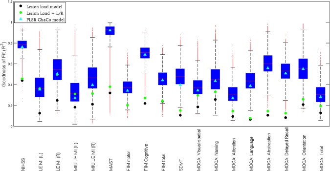
The model fit summary for each clinical assessment NIHSS, LE MI (lower extremity motricity index), UE MI (upper extremity motricity index), MAST, Functional Independence Measure (FIM), SDMT, and MoCA. The R 2 for the linear regression models based on lesion volume are represented by black circles, the R 2 for the linear regression models based on lesion volume and lateralization are represented by green circles, and the R 2 for the fixed‐effects PLSR models based on ChaCo scores are given by cyan triangles. The distribution of R 2 values for the random‐effects bootstrapped PLSR models based on ChaCo are given by boxplots that visualize the median (red line), interquartile range (blue box), range of the most extreme points not considered outliers (black whiskers) and outliers (red points). [Color figure can be viewed in the online issue, which is available at http://wileyonlinelibrary.com.]
“Glassbrain” displays in Figures 3 and 4 visualize the PLSR regression coefficients for regional ChaCo scores. Here, sphere size is proportional to the relative impact of that region's ChaCo score on the clinical assessment. Blue spheres indicate regions whose ChaCo scores significantly increase the value of the predicted outcome (positive coefficients), while red spheres indicate regions that significantly decrease the value of the predicted outcome (negative coefficients). Black spheres indicate regions of nonsignificant influence. The PLSR model components for regional ChaCo are given in Supporting Information Figures II and III, where red indicates negative and blue positive component coefficients. Regression coefficients and component summaries are given in Table 1. Note: the NIHSS was negated before regression to have the same pattern as the other clinical assessments where higher numbers indicate better performance and smaller numbers indicate worse performance.
Figure 3.
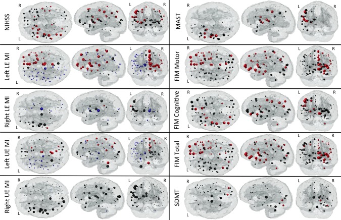
Glassbrain displays visualize the coefficients for the regional ChaCo scores in the PLSR models predicting each outcome variable NIHSS, LE MI (lower extremity motricity index), UE MI (upper extremity motricity index), MAST, Functional Independence Measure (FIM) and Symbol Digits Modality Test (SDMT). Each sphere is located at the center of the GM region it represents. Sphere size is proportional to the relative impact of that region's ChaCo score on the outcome measure. Blue spheres indicate regions whose ChaCo scores significantly increase the value of the predicted outcome (positive coefficients), while red spheres indicate regions that significantly decrease the value of the predicted outcome (negative coefficients). Black spheres indicate regions of nonsignificant influence. [Color figure can be viewed in the online issue, which is available at http://wileyonlinelibrary.com.]
Figure 4.
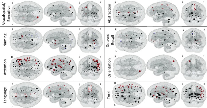
Glassbrain displays visualize the coefficients for the regional ChaCo scores in the PLSR models predicting each subtest outcome in the MOCA. Each sphere is located at the center of the GM region it represents. Sphere size is proportional to the relative impact of that region's ChaCo score on the outcome measure. Blue spheres indicate regions whose ChaCo scores significantly increase the value of the predicted outcome (positive coefficients), while red spheres indicate regions that significantly decrease the value of the predicted outcome (negative coefficients). Black spheres indicate regions of nonsignificant influence. [Color figure can be viewed in the online issue, which is available at http://wileyonlinelibrary.com.]
DISCUSSION
This work has successfully converted neuroimaging observations of structural connectome changes accompanying stroke into a quantitative biomarker of acute post‐stroke impairment based on routine MRI scans. This approach demonstrated robustness in that it produced similar lesion‐dysfunction mapping results for the same functional assessment (the SDMT) across the two disparate pathologies of stroke (here) and multiple sclerosis [Kuceyeski et al., in press]. Additionally, confidence in the veracity of this method's results was bolstered by the fact that it was able to localize eloquent functions to the appropriate areas. Furthermore, this study provides insight into brain structural connectome‐behavior relationships in functions that are less easily mapped, that is, like activities of daily living and cognitive processes that likely depend on distributed brain networks. The presented method, after thorough validation, has the potential to reduce the risk of incorrect prognoses that can accompany subjective radiological assessment. Further modeling of recovery under various treatments could result in a quantitative approach for optimization of individualized rehabilitation plans.
Comparison to Existing Methods for Extracting Brain‐Behavior Relationships
There exist many tools with which to quantify brain‐behavior relationships such as voxel‐based morphometry [Ashburner and Friston, 2000], Tract‐Based Spatial Statistics [Smith et al., 2006], MR volumetrics [Fischl and Dale, 2000; Friston et al., 2006; Ad‐Dab'bagh et al., 2006; Woolrich et al., 2009] and lesion‐symptom mapping [Bates et al., 2003]. Brain atlases that divide WM and GM into anatomically coherent regions have been created [Hua et al., 2008; Oishi et al., 2009; Wakana et al., 2004] and used in lesion‐symptom mapping [Hope et al., 2013]. One drawback of lesion‐mapping approaches is that it considers only the damaged area and does not explicitly take into account the distal affects of lesions in the context of the structural connectome. To our knowledge, the ChaCo score is unique in that it links localized WM lesions' with the corresponding affected GM regions, without having to perform tractography in abnormal subjects. There have been some studies that show relationships between structural connectivity and recovery by performing diffusion imaging [Puig et al., 2013] and tractography [Crofts et al., 2011; Johansen‐Berg et al., 2010] in individual patients. It is not known if tractography methods in these populations can overcome noise from pathology to provide physiologically meaningful connectivity information, see discussion in Crofts et al., [2011]. While these studies do provide important insights into the mechanisms of recovery in regions not obviously affected by the stroke lesion, it is not as accurate in areas proximal to the lesion. More importantly, it is difficult to perform high‐quality diffusion MRI needed for these types of analysis in the acute clinical setting. We argue that the ChaCo score can be a good substitute for, and at times more accurate than, performing diffusion imaging and tractography in patient populations.
Many other studies have used lesion‐mapping approaches to link structure to function [Hope et al., 2013; Mort et al., 2003]. However, the functions are usually restricted to specific domains like language, motor and some areas of cognition [Barbey et al., 2012; Butler et al., 2014; Gläscher et al., 2010; Hope et al., 2013; Phan et al., 2010], in lieu of more complex and general behaviors like activities of daily living that may be integral when developing patient prognoses. Here, we present a machine learning approach that can assess brain‐behavior relationships across many different and quite variable domains, from specific to general, with strict controls for multiple comparisons correction. This method also considers the continuous nature of functional measures as opposed to dividing function into “impaired” and “not impaired” groups, as many studies have previously performed [Counsell et al., 2002; Pedersen et al., 1995].
Comparison to Previously Identified Brain‐Behavior Relationships
Uniformly, NeMo/PLSR models based on ChaCo scores had higher goodness‐of‐fit and lower AIC than models based on lesion volume. As anticipated, adding lateralization information to lesion volume models increased the goodness‐of‐fit for predictions of motor function to values similar to the NeMo/PLSR models. However, AIC values were still smaller in the NeMo/PLSR models due to the larger number of input variables. Many regions in eloquent cortices were identified as significant predictors of the known corresponding behavior and served to validate the NeMo/PLSR approach. For example, lesions in right motor areas predicted worse performance on left MI and vice versa. Moreover, lesions affecting connectivity of Broca's areas, left frontal operculum and areas related to facial, tongue and lip movement were predictors of aphasia [Alexander et al., 1990]. However, the current analysis may be particularly enlightening when determining the contribution of noneloquent cortices to complex behaviors requiring more distributed brain input, such as attention, memory and daily life activities.
Areas with language and motor functions, central to the NIHSS, were significant predictors of individuals' scores, with a slight emphasis on left regions. Higher age was associated with smaller NIHSS; in fact, there existed a positive and significant Pearson correlation between negated NIHSS and age (r = 0.32, P<0.05). This observation may be a result of the subject selection criteria, as older subjects with higher NIHSS may not have met the criteria or survived to be admitted to the rehabilitation unit. We observed that lower NIHSS values were not as well predicted with our model (Supporting Information Figure I). This is most likely due to the nonlinear nature of the score for less severe strokes [Fonarow et al., 2012], which may be better predicted using logistic PLSR[Phan et al., 2010].
In general, coefficients that predicted a subject's FIM scores were less localized than other tests. This may be due to the complex nature of the tasks of the FIM, for example, locomotion, eating, grooming, dressing, cognitive comprehension, expression, social interaction and problem solving that likely require distributed input from various brain networks. In the prediction of FIM motor, ChaCo in orbital‐frontal areas that deal with executive functions, emotion and decision‐making [Fuster, 2008] had the largest coefficients. The right hippocampus, also important to FIM motor, was shown to be important in linking an action to its consequences [Elsner et al., 2002]. Other studies have identified the hippocampus as an important factor in navigation [Maguire, 1998] and locomotive control, particularly in the acute phase [Vanderwolf, 2001]. PLSR model predictions of FIM have a ceiling effect (Supporting Information Figure I), indicating possible model insensitivity for these values. This may be remedied by adding to the model other important demographic information, for example, previous independence level.
The SDMT, requiring close visual attention and memory recall, was predicted by ChaCo in right occipital areas that deal with visual processing and attention. In a similar study of multiple sclerosis subjects, we also found using ChaCo scores that higher burden of T2‐FLAIR hyperintesities in WM connecting to occipital and bordering parietal regions was significantly related to worse SDMT performance[Kuceyeski et al., in press]. This robust observation across pathology states, image parameters, and data collection sites not only strengthens our belief in the physiological finding, but also serves to validate the current methodology.
Significant predictors of the MOCA visual‐spatial/executive subscore included parietal regions that are critical to spatial awareness, hand‐eye coordination, vision, and somatosensory processing [Bear et al., 2006]. This subtest involves drawing a clock and copying a cube, both of which require these functions in addition to executive planning. Previous work [Corbetta and Shulman, 2002] identified an inferior frontal‐temporal‐parietal network in the right hemisphere that was specialized in the detection of behaviorally relevant stimuli; this exact network contributed to prediction of attention scores. Regions that were significant predictors of language and abstraction subscores were medial, that is, anterior and middle cingulate and medial frontal areas. Cingulate structures have been shown to play a role in emotion formation, learning and memory [Stanislav et al., 2013], which may explain their importance here. Bilateral prefrontal regions and the globus pallidus that were significant in the delayed recall task have been shown to be activated in recall and recognition tasks [Cabeza et al., 2003]. Language, abstraction and delayed recall tasks, all having a central verbal component, had similar patterns of regression coefficients that did not involve left hemispheric language‐related regions. Most likely these complex tasks require proper functioning of multiple distributed networks, that is, attention, vision, and memory, which makes mapping them more difficult. A larger and more varied population is needed to fully understand the relationship between structure and these complex functions. Total MOCA was predicted with the lowest goodness‐of‐fit, possibly due to it being a combination of all subscores, each in turn being related to a localized, distinct network. Indeed, total MOCA regression coefficients appear distributed over the entire brain (Figure 4), but only those in the right attention network survived significance testing.
There were some seemingly unanticipated results showing higher ChaCo was associated with better performance on certain clinical assessments. However, these instances most likely arise either from noise in the data and model (see Limitations), or are not surprising on further inspection. For example, higher ChaCo in left motor areas was correlated with better scores on the left MI and vice versa. This phenomena can be explained thus: if a person had a lesion in the left motor area (higher ChaCo in left motor regions) then they most likely did not have a lesion in the right motor area and thus did not have impairment of left motor function (better scores on left MI).
Limitations and Future Work
Models built with too few data points are subject to over‐fitting to that particular data set. Here, over‐fitting was minimized by cross‐validation and bootstrapping techniques for model building and performance assessment. Even so, models were limited by the characteristics of the available population. For example, if there was an important WM connection for a particular function that was not affected in any of the stroke subjects, then it was not detected by the model. Future work will be needed as more data becomes available. This analysis also did not investigate long‐term recovery, which may be more important clinically. Detailed measures of recovery are currently being collected in these same subjects 6 and 12 months poststroke. Future work will focus on long‐term prediction of recovery from MRI‐based imaging biomarkers to inform prognosis and possibly rehabilitation plan development.
There are potential sources of error in the current processing pipeline that arises from the lesion masking process and varying image acquisition parameters over the population. There are strengths and weaknesses for automated thresholding methods versus the hand‐drawn lesion approach used here, which was shown to have adequate Dice's inter‐rater coefficient. With either method, some manual editing is needed to deal with phenomena like T2 shine through, partial volume effects and other possible artifacts. Since these are difficult to manage by purely automated analyses, there is some justification for the hand‐drawn approach that is informed by image intensity but uses more of the available information. Therefore, we chose to manually outline the areas of hyperintensity on the DWI. Pre‐existing tissue abnormalities, including periventricular DWI hyperintensities from T2 shine‐through, were excluded when creating the lesion masks. While chronic pathologies may influence a subject's scores of clinical dysfunction, this relationship most likely depends on the age of the lesion. Since aging a chronic lesion is impossible and we wanted to focus on the influence of the acute lesion only, we decided to leave these variables out of the model. Future studies could aim to somehow quantify and characterize pre‐existing abnormalities in addition to the acute infarct. In addition, T1‐ versus T2‐based normalization effects were shown to be minimal in a study of similar patients [Kuceyeski et al., 2014]. Furthermore, a recent study illustrating bias introduced by the structure of the vascular tree and the erroneous assumption of independence of individual voxels may present an issue for lesion‐mapping studies in stroke [Mah et al., 2014]. However, those particular issues are somewhat mitigated here since we investigate at network disruption on a regional basis, which is likely less influenced by such biased assumptions.
Some measures, in particular NIHSS, clinical assessments with categorical outcomes or those that tend to have a ceiling effect like motoricity index, may be better predicted with a nonlinear approach like logistic PLSR. Because we wanted to exploit the continuous nature of the functional assessments, we did not implement such an approach here. In the future, however, we will investigate the application of these methods when predicting measures for which the standard PLSR model is determined inadequate.
The rise of big data and machine learning approaches in neuroscience through the cooperation of multiple collection sites will be central to understanding these complex brain‐behavior relationships. Similar to the 1,000 connectomes project [Biswal et al., 2010] and the Human Connectome Project [Van Essen et al., 2012] that collect neuroimaging and behavioral data in healthy subjects, we advocate the creation of a “1000 Lesions Project”. This project would represent a large‐scale effort to create big data sets that contain both neuroimaging and wide‐ranging behavioral data for subjects with brain lesions. Subjects with ischemic stroke represent a sensible choice—such subjects are not rare, most likely have compromised regions that can be easily delineated, and already undergo imaging as a part of standard medical care. However, the generalizability of the mostly older stroke population and issues with bias in stroke lesion‐mapping [Mah et al., 2014] may necessitate the use of other populations in the dataset. Multiple Sclerosis or Cerebral Autosomal‐Dominant Arteriopathy with Subcortical Infarcts and Leukoencephalopathy subjects could be included in the database to investigate consistencies across pathologies. Whatever the population, the aims of this proposed database would be twofold. Behavioral data collected acutely can help us better understand brain‐behavior relationships while longitudinally collected data of both dysfunction and intervention may help us to improve prognostic tools and possibly develop individualize treatment plans.
Conclusions
Here, we use a machine learning approach on a moderately sized data set of both neuroimaging and wide‐ranging behavioral data to identify possible brain structural connectome‐behavior relationships. We have shown that the NeMo Tool's quantitative assessment of structural connectome disruption due to infarct allows prediction of an individual's acute impairment and ability in several domains. Models of eloquent functions, that is, language and motor, provided validation of the method, while models of more complex behavioral measures provided new insights into brain‐behavior relationships. Robustness of this method was demonstrated in the replication of connectome‐behavior relationships for a particular function across pathologies. The fact that this method can be applied on clinically acquired neuroimaging data gives it an advantage over other methods. In addition to the possible application of improving the accuracy of poststroke prognoses, the current analysis offers the opportunity to gain insight into the neural substrates underlying complex behaviors such as those associated with activities of daily living and specific areas of cognition.
Supporting information
Supporting Information
Supporting Information
Supporting Information
REFERENCES
- Alexander MP, Naeser MA, Palumbo C (1990): Broca's area aphasias: Aphasia after lesions including the frontal operculum. Neurology 40:353–362. [DOI] [PubMed] [Google Scholar]
- Ashburner J, Friston KJ (2000): Voxel‐based morphometry–the methods. Neuroimage 11:805–821. [DOI] [PubMed] [Google Scholar]
- Barbey AK, Colom R, Solomon J, Krueger F, Forbes C, Grafman J (2012): An integrative architecture for general intelligence and executive function revealed by lesion mapping. Brain 135:1154–1164. [DOI] [PMC free article] [PubMed] [Google Scholar]
- Bates E, Wilson S, Saygin A, Dick F, Sereno M, Knight R, Dronkers N (2003): Voxel‐based lesion‐symptom mapping. Nat Neurosci 6:448–450. [DOI] [PubMed] [Google Scholar]
- Bear M, Connors B, Paradiso M (2006): Neuroscience: Exploring the Brain, 3rd ed Lippincott Williams & Wilkins; Baltimore, MD: [Google Scholar]
- Biswal BB, Mennes M, Zuo X‐N, Gohel S, Kelly C, Smith SM, Beckmann CF, Adelstein JS, Buckner RL, Colcombe S, Dogonowski A‐M, Ernst M, Fair D, Hampson M, Hoptman MJ, Hyde JS, Kiviniemi VJ, Kötter R, Li S‐J, Lin C‐P, Lowe MJ, Mackay C, Madden DJ, Madsen KH, Margulies DS, Mayberg HS, McMahon K, Monk CS, Mostofsky SH, Nagel BJ, Pekar JJ, Peltier SJ, Petersen SE, Riedl V, Rombouts SARB, Rypma B, Schlaggar BL, Schmidt S, Seidler RD, Siegle GJ, Sorg C, Teng G‐J, Veijola J, Villringer A, Walter M, Wang L, Weng X‐C, Whitfield‐Gabrieli S, Williamson P, Windischberger C, Zang Y‐F, Zhang H‐Y, Castellanos FX, Milham MP (2010): Toward discovery science of human brain function. Proc Natl Acad Sci USA 107:4734–4739. [DOI] [PMC free article] [PubMed] [Google Scholar]
- Broca P (1861): Remarques sur le siège de la faculté du langage articulé; suivies d'une observation d'aphémie (perte de la parole). Bull la Société Anat Paris 35:330–357. [Google Scholar]
- Brott T, Adams HP, Olinger CP, Marler JR, Barsan WG, Biller J, Spilker J, Holleran R, Eberle R, Hertzberg V (1989): Measurements of acute cerebral infarction: A clinical examination scale. Stroke 20:864–870. [DOI] [PubMed] [Google Scholar]
- Burnham K, Anderson D (2002): Model Selection and Multimodal Inference, 2nd ed New York, NY: Springer‐Verlag. [Google Scholar]
- Butler RA, Ralph MAL, Woollams AM (2014): Capturing multidimensionality in stroke aphasia: Mapping principal behavioural components to neural structures. Brain 137:3248–3266. [DOI] [PMC free article] [PubMed] [Google Scholar]
- Cabeza R, Locantore JK, Anderson ND (2003): Lateralization of prefrontal activity during episodic memory retrieval: Evidence for the production‐monitoring hypothesis. J Cogn Neurosci 15:249–259. [DOI] [PubMed] [Google Scholar]
- Collin C, Wade D (1990): Assessing motor impairment after stroke: A pilot reliability study. J Neurol Neurosurg Psychiatry 53:576–579. [DOI] [PMC free article] [PubMed] [Google Scholar]
- Corbetta M, Shulman GL (2002): Control of goal‐directed and stimulus‐driven attention in the brain. Nat Rev Neurosci 3:201–215. [DOI] [PubMed] [Google Scholar]
- Counsell C, Dennis M, McDowall M, Warlow C (2002): Predicting outcome after acute and subacute stroke: Development and validation of new prognostic models. Stroke 33:1041–1047. [DOI] [PubMed] [Google Scholar]
- Crofts JJ, Higham DJ, Bosnell R, Jbabdi S, Matthews PM, Behrens TEJ, Johansen‐Berg H (2011): Network analysis detects changes in the contralesional hemisphere following stroke. Neuroimage 54:161–169. [DOI] [PMC free article] [PubMed] [Google Scholar]
- Fischl B, Dale AM (2000): Measuring the thickness of the human cerebral cortex from magnetic resonance images. Proc Natl Acad Sci 97:11050–11055. [DOI] [PMC free article] [PubMed] [Google Scholar]
- Dunn OJ (1961): Multiple Comparisons among means. J Am Stat Assoc 56:52–64. [Google Scholar]
- Efron B (1987): Better bootstrap confidence intervals. J Am Stat Assoc 82:171–185. [Google Scholar]
- Elsner B, Hommel B, Mentschel C, Drzezga A, Prinz W, Conrad B, Siebner H (2002): Linking actions and their perceivable consequences in the human brain. Neuroimage 17:364–372. [DOI] [PubMed] [Google Scholar]
- Fonarow GC, Saver JL, Smith EE, Broderick JP, Kleindorfer DO, Sacco RL, Pan W, Olson DM, Hernandez AF, Peterson ED, Schwamm LH (2012): Relationship of national institutes of health stroke scale to 30‐day mortality in medicare beneficiaries with acute ischemic stroke. J Am Heart Assoc 1:42–50. [DOI] [PMC free article] [PubMed] [Google Scholar]
- Friston KJ, Ashburner JT, Kiebel SJ, Nichols TE, Penny WD (2006): Statistical Parametric Mapping: The Analysis of Functional Brain Images. Academic Press; London, UK. [Google Scholar]
- Fuster J (2008): The Prefrontal Cortex, 4th ed Academic Press; London, UK. [Google Scholar]
- Gläscher J, Rudrauf D, Colom R, Paul LK, Tranel D, Damasio H, Adolphs R (2010): Distributed neural system for general intelligence revealed by lesion mapping. Proc Natl Acad Sci USA 107:4705–4709. [DOI] [PMC free article] [PubMed] [Google Scholar]
- Hay JF, Kane KA, West R, Alain C (2002): Event‐related neural activity associated with habit and recollection. Neuropsychologia 40:260–270. [DOI] [PubMed] [Google Scholar]
- Hope TMH, Seghier ML, Leff AP, Price CJ (2013): Predicting outcome and recovery after stroke with lesions extracted from MRI images. NeuroImage Clin 2:424–433. [DOI] [PMC free article] [PubMed] [Google Scholar]
- Hua K, Zhang J, Wakana S, Jiang H, Li X, Reich DS, Calabresi PA, Pekar JJ, Van Zijl PCM, Mori S (2008): Tract probability maps in stereotaxic spaces: analyses of white matter anatomy and tract‐specific quantification. Neuroimage 39:336–347. [DOI] [PMC free article] [PubMed] [Google Scholar]
- Itier RJ, Taylor MJ, Lobaugh NJ (2004): Spatiotemporal analysis of event‐related potentials to upright, inverted, and contrast‐reversed faces: Effects on encoding and recognition. Psychophysiology 41:643–653. [DOI] [PubMed] [Google Scholar]
- Ad‐Dab'bagh Y, Einarson D, Lyttelton O, Muehlboeck JS, Mok K, Ivanov O, Vincent RD, Lepage C, Lerch J, Fombonne E, Evans AC (2006): The CIVET image‐processing environment: A fully automated comprehensive pipeline for anatomical neuroimaging research. Proceedings of the 12th Annual Meeting of the Organization for Human Brain Mapping. [Google Scholar]
- Johansen‐Berg H, Scholz J, Stagg CJ (2010): Relevance of structural brain connectivity to learning and recovery from stroke. Front Syst Neurosci 4:146. [DOI] [PMC free article] [PubMed] [Google Scholar]
- Keith RA, Granger C V, Hamilton BB, Sherwin FS (1987): The functional independence measure: A new tool for rehabilitation. Adv Clin Rehabil 1:6–18. [PubMed] [Google Scholar]
- Krishnan A, Williams LJ, McIntosh AR, Abdi H (2011): Partial Least Squares (PLS) methods for neuroimaging: A tutorial and review. Neuroimage 56:455–475. [DOI] [PubMed] [Google Scholar]
- Kuceyeski A, Maruta J, Niogi SN, Ghajar J, Raj A (2011): The generation and validation of white matter connectivity importance maps. Neuroimage 58:109–121. [DOI] [PMC free article] [PubMed] [Google Scholar]
- Kuceyeski A, Maruta J, Relkin N, Raj A (2013): The Network Modification (NeMo) Tool: Elucidating the effect of white matter integrity changes on cortical and subcortical structural connectivity. Brain Connect 3:451–463. [DOI] [PMC free article] [PubMed] [Google Scholar]
- Kuceyeski A, Kamel H, Navi BB, Raj A, Iadecola C (2014): Predicting future brain tissue loss from white matter connectivity disruption in ischemic stroke. Stroke 45:717–722. [DOI] [PMC free article] [PubMed] [Google Scholar]
- Kuceyeski A, Dayan M, Vargas W, Monohan E, Blackwell C, Raj A, Fujimoto K, Gauthier S: Modeling the relationship between gray matter atrophy, abnormalities in connecting white matter and cognitive performance in early Multiple Sclerosis (in press). [DOI] [PMC free article] [PubMed]
- Maguire EA (1998): Knowing where and getting there: A human navigation network. Science 280:921–924. [DOI] [PubMed] [Google Scholar]
- Mah Y‐H, Husain M, Rees G, Nachev P (2014): Human brain lesion‐deficit inference remapped. Brain 137:2522–2531. [DOI] [PMC free article] [PubMed] [Google Scholar]
- Menezes NM, Ay H, Wang Zhu M, Lopez CJ, Singhal AB, Karonen JO, Aronen HJ, Liu Y, Nuutinen J, Koroshetz WJ, Sorensen AG (2007): The real estate factor: Quantifying the impact of infarct location on stroke severity. Stroke 38:194–197. [DOI] [PubMed] [Google Scholar]
- Milner B (1982): Some cognitive effects of frontal‐lobe lesions in man. Philos Trans R Soc B Biol Sci 298:211–226. [DOI] [PubMed] [Google Scholar]
- Mort DJ, Malhotra P, Mannan SK, Rorden C, Pambakian A, Kennard C, Husain M (2003): The anatomy of visual neglect. Brain 126:1986–1997. [DOI] [PubMed] [Google Scholar]
- Nakase‐Thompson R, Manning E, Sherer M, Yablon SA, Gontkovsky SLT, Vickery C (2005): Brief assessment of severe language impairments: Initial validation of the Mississippi aphasia screening test. Brain Inj 19:685–691. [DOI] [PubMed] [Google Scholar]
- Nasreddine ZS, Phillips NA, Bédirian V, Charbonneau S, Whitehead V, Collin I, Cummings JL, Chertkow H (2005): The Montreal Cognitive Assessment, MoCA: A brief screening tool for mild cognitive impairment. J Am Geriatr Soc 53:695–699. [DOI] [PubMed] [Google Scholar]
- Oishi K, Faria A, Jiang H, Li X, Akhter K, Zhang J, Hsu JT, Miller MI, van Zijl PCM, Albert M, Lyketsos CG, Woods R, Toga AW, Pike GB, Rosa‐Neto P, Evans A, Mazziotta J, Mori S (2009): Atlas‐based whole brain white matter analysis using large deformation diffeomorphic metric mapping: Application to normal elderly and Alzheimer's disease participants. Neuroimage 46:486–499. [DOI] [PMC free article] [PubMed] [Google Scholar]
- Pagani E, Bammer R, Horsfield MA, Rovaris M, Gass A, Ciccarelli O, Filippi M (2007): Diffusion MR Imaging in Multiple Sclerosis: Technical Aspects and Challenges. AJNR Am J Neuroradiol 28:411–420. [PMC free article] [PubMed] [Google Scholar]
- Pedersen PM, Jørgensen HS, Nakayama H, Raaschou HO, Olsen TS (1995): Aphasia in acute stroke: incidence, determinants, and recovery. Ann Neurol 38:659–666. [DOI] [PubMed] [Google Scholar]
- Phan TG, Chen J, Donnan G, Srikanth V, Wood A, Reutens DC (2010): Development of a new tool to correlate stroke outcome with infarct topography: A proof‐of‐concept study. Neuroimage 49:127–133. [DOI] [PubMed] [Google Scholar]
- Posner M, Petersen S, Fox P, Raichle M (1988): Localization of cognitive operations in the human brain. Science 240:1627–1631. [DOI] [PubMed] [Google Scholar]
- Puig J, Blasco G, Daunis‐I‐Estadella J, Thomalla G, Castellanos M, Figueras J, Remollo S, van Eendenburg C, Sánchez‐González J, Serena J, Pedraza S (2013): Decreased corticospinal tract fractional anisotropy predicts long‐term motor outcome after stroke. Stroke 44:2016–2018. [DOI] [PubMed] [Google Scholar]
- Smith A (1982): Symbol Digits Modality Test. Western Psychological Services, Los Angeles, CA.
- Smith SM, Jenkinson M, Johansen‐Berg H, Rueckert D, Nichols TE, Mackay CE, Watkins KE, Ciccarelli O, Cader MZ, Matthews PM, Behrens TEJ (2006): Tract‐based spatial statistics: voxelwise analysis of multi‐subject diffusion data. Neuroimage 31:1487–1505. [DOI] [PubMed] [Google Scholar]
- Stanislav K, Alexander V, Maria P, Evgenia N, Boris V (2013): Anatomical characteristics of cingulate cortex and neuropsychological memory tests performance. Procedia—Soc Behav Sci 86:128–133. [Google Scholar]
- Tzourio‐Mazoyer N, Landeau B, Papathanassiou D, Crivello F, Etard O, Delcroix N, Mazoyer B, Joliot M (2002): Automated anatomical labeling of activations in SPM using a macroscopic anatomical parcellation of the MNI MRI single‐subject brain. Neuroimage 15:273–289. [DOI] [PubMed] [Google Scholar]
- Vanderwolf C. (2001): The hippocampus as an olfacto‐motor mechanism: Were the classical anatomists right after all? Behav Brain Res 127:25–47. [DOI] [PubMed] [Google Scholar]
- Van Essen DC, Ugurbil K, Auerbach E, Barch D, Behrens TEJ, Bucholz R, Chang A, Chen L, Corbetta M, Curtiss SW, Della Penna S, Feinberg D, Glasser MF, Harel N, Heath AC, Larson‐Prior L, Marcus D, Michalareas G, Moeller S, Oostenveld R, Petersen SE, Prior F, Schlaggar BL, Smith SM, Snyder AZ, Xu J, Yacoub E (2012): The Human Connectome Project: A data acquisition perspective. Neuroimage 62:2222–2231. [DOI] [PMC free article] [PubMed] [Google Scholar]
- Van Hees S, McMahon K, Angwin A, de Zubicaray G, Read S, Copland DA (2014): Changes in white matter connectivity following therapy for anomia post stroke. Neurorehabil Neural Repair 28:325–334. [DOI] [PubMed] [Google Scholar]
- Wakana S, Jiang H, Nagae‐Poetscher LM, van Zijl PCM, Mori S (2004): Fiber tract‐based atlas of human white matter anatomy. Radiology 230:77–87. [DOI] [PubMed] [Google Scholar]
- Wernicke C (1874): Der aphasische Symptomencomplex: Eine psychologische Studie auf anatomischer Basis. Breslau: Max Cohn & Weigert. [Google Scholar]
- Wheeler‐Kingshott CAM, Cercignani M (2009): About “axial” and “radial” diffusivities. Magn Reson Med 61:1255–1260. [DOI] [PubMed] [Google Scholar]
- Wold H (1982): Soft modeling: the basic design and some extensions. Syst under Indirect Obs 2:589–591. [Google Scholar]
- Wold S, Ruhe A, Wold H, Dunn, III WJ (1984): The Collinearity problem in linear regression. The partial least squares (PLS) approach to generalized inverses. SIAM J Sci Stat Comput 5:735–743. [Google Scholar]
- Woolrich MW, Jbabdi S, Patenaude B, Chappell M, Makni S, Behrens T, Beckmann C, Jenkinson M, Smith SM (2009): Bayesian analysis of neuroimaging data in FSL. Neuroimage 45:S173–S186. [DOI] [PubMed] [Google Scholar]
Associated Data
This section collects any data citations, data availability statements, or supplementary materials included in this article.
Supplementary Materials
Supporting Information
Supporting Information
Supporting Information