Quantification of Tumor Burden in a Genetically Engineered Mouse Model of Lung Cancer by Micro-CT and Automated Analysis

Abstract

Genetically engineered mouse models (GEMMs) of lung cancer closely recapitulate the human disease but suffer from the difficulty of evaluating tumor growth by conventional methods. Herein, a novel automated image analysis method for estimating the lung tumor burden from in vivo micro-computed tomography (micro-CT) data is described. The proposed tumor burden metric is the segmented soft tissue volume contained within a chest space region of interest, excluding an estimate of the heart volume. The method was validated by comparison with previously published manual analysis methods and applied in two therapeutic studies in a mutant K-ras GEMM of non–small cell lung carcinoma. Mice were imaged by micro-CT pre-treatment and stratified into four treatment groups: an antibody inhibiting vascular endothelial growth factor (anti-VEGF), chemotherapy, combination of anti-VEGF and chemotherapy, or control antibody. In the first study, post-treatment imaging was performed 4 weeks later. In the second study, mice were scanned serially on a high-throughput scanner every 2 weeks for 8 weeks during treatment. In both studies, the automated tumor burden estimates were well correlated with manual metrics (r value range: 0.83-0.93, P < .0001) and showed a similar, significant reduction in tumor growth in mice treated with anti-VEGF alone or in combination with chemotherapy. Given the fully automated nature of this technique, the proposed analysis method can provide a valuable tool in preclinical drug research for screening and randomizing animals into treatment groups and evaluating treatment efficacy in mouse models of lung cancer in a highly robust and efficient manner.

Introduction

Lung cancer causes more deaths worldwide than any other cancer type [1,2]. Development of novel therapies to battle lung cancer has been greatly aided by the emergence of genetically engineered mouse models (GEMMs) of lung cancer, such as the K-ras^G12D;p53^Frt/Frt non–small cell lung carcinoma (NSCLC) model [3], where the compound effect of conditional mutations in the K-ras oncogene and the p53 tumor suppressor gene leads to development of adenocarcinomas in the mouse lung [4]. GEMMs recapitulate certain aspects of the human disease associated with the stroma, vascularity, and immune infiltrate more closely than xenograft models, where tumor cell lines are implanted in immunocompromised animals [5,6]. However, detection of a therapeutic effect by candidate treatments in these models is difficult by traditional means. Unlike subcutaneous xenografts, the GEMM lung tumors are not measurable by an external caliper. Histologic evaluation is time-consuming, spatially limited within the selected slices, and cannot provide knowledge about the baseline tumor burden in individual animals before the treatment is started.

In the clinical setting, computed tomography (CT) is widely used for detection of lung tumors [7,8]. Image intensities in CT are quantitative and proportional to the tissue density, which results in good contrast between solid tumors and the air space (including airways and alveolar tissue). Micro-CT, which offers higher resolution than clinical CT systems, has been successfully used for detecting lung tumors and evaluating tumor burden in mouse lung cancer models, including preclinical studies of NSCLC GEMMs [3,9–15]. Serial in vivo imaging of the animals during a treatment study has several advantages by offering a non-invasive method of screening, randomizing animals into treatment groups based on baseline tumor burden, and enabling quantification of treatment effects on tumor load at different time points within the same animals. Previously reported methods for quantifying the tumor burden from micro-CT data have relied on some form of manual input for every image [3,12]. This typically makes an analysis method time-consuming, vulnerable to intra-reader and inter-reader variability and potential reader bias, and generally requires identification of the tumor tissue by the reader. Semi-automated methods [16–19] have been reported for segmenting and tracking individual lung nodules, but there remains a need for a time-efficient method for quantifying lung tumor burden in a robust manner. Fully automating the image analysis would offer significant benefits in drug development studies where objective and reproducible quantification of the tumor burden is crucial, and high throughput is necessary for gaining statistical power.

What makes the automation of micro-CT image analysis in the K-ras mutant;p53 null model challenging is the vast range of tumor burden during the course of a study [4,12]. The tumor tissue is indistinguishable by image intensities from other soft tissues in the thoracic cavity, such as heart, diaphragm, and blood vessels. With increasing tumor burden, the individual tumors become connected with other tissues and even manual differentiation of the tumors by a trained reader becomes challenging. In this study, a novel automated tumor burden quantification method is introduced. The method does not rely on differentiation of soft tissue lesions but rather works by automatically identifying a consistent region within the rib cage for monitoring changes in the soft tissue content over time. To account for differences in the heart size between subjects and time points, a correction is applied in the soft tissue volume calculation by automatically estimating the heart volume from the image data and removing it from the total soft tissue volume. The automated analysis method was validated against a previously validated manual tumor cross-product analysis method [3] and a semi-automated volumetric analysis method proposed by Haines et al. [12]. The new automated method was also applied to a study that was performed on a high-throughput micro-CT system. Both studies demonstrated the method’s capability of detecting a treatment effect of anti-angiogenic therapy by monoclonal antibodies that inhibit vascular endothelial growth factor (VEGF) A in a GEMM of NSCLC. An anti-VEGF antibody, bevacizumab (Avastin), in combination with chemotherapy is used as a standard of care for advanced NSCLC.

Materials and Methods

Genetically Engineered Mouse Model

K-ras^LSL-G12D;p53^Frt/Frt positive animals were generated as previously described [3] and maintained on a C57Bl/6J-Tyr strain background. Tumors were induced in the K-ras^LSL-G12D;p53^Frt/Frt mice by infection with 5 × 10⁶ infectious units of Adeno-FLPe/IRES/CRE at 7 to 9 weeks of age. At 16 weeks post-infection, mice were randomized into treatment groups based on micro-CT tumor burden estimates, body weights, and gender. All animals were dosed and monitored according to the guidelines from the Institutional Animal Care and Use Committee at Genentech, Inc (South San Francisco, CA). All dosing regimens were well tolerated, with no significant body weight loss or overt signs of toxicity other than those attributable to the disease itself.

Validation Study

Treatment regimen

Mice in the validation study were dosed as previously described [3]. Anti-VEGF (B20-4.1.1, mouse IgG2a) and control (anti-ragweed, mouse IgG2a) antibodies were prepared and purified at Genentech, Inc. Antibodies were dosed through intraperitoneal injection at 5 mg/kg twice weekly until the end of study. Chemotherapy (carboplatin: Paraplatin from Bristol-Myers Squibb, New York, NY, or generic from Pliva d.d., Zagreb, Croatia.) was dosed intraperitoneally at 25 mg/kg for the first 5 days of the study. The treatment groups were control (n = 9), chemo (n = 10), anti-VEGF (n = 9), and anti-VEGF + chemo (n = 8).

Micro-CT scanning

Micro-CT was performed pre-treatment and 4 weeks after the start of treatment as described [3]. Briefly, serial lung imaging was performed on an in vivo micro-CT system (vivaCT 40; Scanco Medical, Bruettisellen, Switzerland). Data were acquired at 38-μm isotropic voxel size, 1000 projections, 250-ms integration time, 45-keV photon energy, and 177-μA current. During in vivo imaging, the animals were anesthetized with 2% isoflurane in medical air and kept at a constant 37°C temperature by regulated warm airflow. The imaging time at each time point was approximately 25 minutes per animal, and the estimated radiation dose was 0.2 Gy.

High-Throughput Serial Study

Treatment regimen

Mice in the high-throughput serial study were dosed similarly to the validation study, with the following exception: chemotherapy (carboplatin) was given at 60 mg/kg every 4 days for six doses. The treatment groups were control (n = 9), chemo (n = 9), anti-VEGF (n = 9), and anti-VEGF + chemo (n = 9).

Micro-CT scanning

Micro-CT was performed pre-treatment and 2, 4, 6, and 8 weeks after the start of treatment. The mice were scanned on an in vivo micro-CT system (eXplore CT120; Trifoil Imaging, Chatsworth, CA) using an in-house built animal holder that allows four mice to be scanned simultaneously. The scanning parameters were 900 projections per full rotation, 16-ms integration time, 75-keV photon energy, 40-mA tube current, and 4 × 4 detector binning. The lung images from the four mice were reconstructed within individual regions of 275 × 275 × 300 voxels and 100-μm isotropic voxel size. The animals were anesthetized with 2% isoflurane in medical air, and the scan time was approximately 5 minutes per four mice resulting in an average scan time of 1.25 minutes per mouse.

Data Analysis

The image analysis methods for data from the two different scanners are essentially identical but accommodate for scanner-dependent differences in image intensities, voxel dimensions, and smoothness of the images where applicable. The micro-CT image intensities were converted to Hounsfield units (HU) according to the scanner manufacturers’ calibration methods. For intensity thresholding procedures, the threshold values were chosen empirically to optimize algorithm performance and differ somewhat between the scanners. Scanner-dependent differences in HU values are commonly caused by differences in the X-ray energy spectrum, the scanner geometry, and the detector’s non-linearity [20,21].

Cross-Product Analysis

The manual cross-product analysis of micro-CT images for tumor burden quantification was performed as described previously [3]. Image data were evaluated using Analyze image analysis software (AnalyzeDirect, Lenexa, KS). The lung micro-CT data were viewed in the coronal plane to identify tumors. The largest cross-sectional plane of each tumor was determined by the reader, from which estimates of maximal tumor diameter (d₁) and the largest perpendicular diameter (d₂) were determined by placing a ruler on the screen. The total tumor burden was defined as the sum of the cross-products (SCP) of the directional estimates of all tumors per animal: SCP = ∑(d₁ × d₂). This in vivo micro-CT tumor analysis method has been previously validated by ex vivo micro-CT analysis [3].

Tracing Analysis

The tumor burden was also quantified with a manual tracing method of micro-CT images that was based on a previously proposed method by Haines et al. [12]. The total intra-thoracic space within the rib cage, excluding heart, mediastinum, liver, and diaphragm, was segmented with Analyze software by manually drawing regions in the transverse plane on approximately eight evenly spaced slices and propagating (linear interpolation) between the regions to include all slices in the region of interest (ROI).

Soft, non-alveolar tissue was automatically segmented as follows: The image data from the vivaCT 40 scanner were low-pass filtered by a 3 × 3 × 3 mean filter, intensity-thresholded, and morphologically filtered (opened and closed with a 3 × 3 × 3 kernel) [22]. The image data from the eXplore CT120 were segmented by intensity thresholding only. The threshold range for the segmentation was chosen empirically based on visual inspection of a small set of animals (vivaCT 40: − 260 to 580 HU, eXplore CT120: − 280 to 100 HU). The soft tissue was then masked with the ROI to calculate the tumor and vasculature volume (TVV). Since the vascular portion of TVV is expected to remain relatively constant, changes in TVV are expected to predominantly stem from tumor growth or regression.

Automated Analysis

The automated image analysis algorithm for estimating the lung tumor burden was written in C++ language using the AVW function libraries (AnalyzeDirect) and was based on intensity thresholding and morphologic operations. An overview of the method is presented in Figure 1. The guiding principle is to automatically identify a consistent ROI bounded by anatomic landmarks, so that the same region of the lung is included in the ROI even if the lung shape or size changes, which can occur due to lung expansion associated with greater tumor burden. The ROI is confined to be within the rib cage in the transverse plane and between the tracheal bifurcation (TB) and the interface between the heart and the diaphragm in the axial direction. Soft tissue is then segmented within the ROI by employing the same thresholding values and morphologic filtering as described above for the tracing analysis. The goal was also to eliminate variability in the amount of included non-tumor tissue. Since the heart is a major component of the soft tissue within the ROI, an algorithm was developed to estimate the included heart volume, which is then subtracted from the total tissue volume. The specific steps of the algorithm are described below in the following sections.

Figure 1.

Automated image analysis method for lung tumor burden quantification. The flowchart illustrates the main steps of the method, starting with the original micro-CT image of the lung. The 3D ROI is bounded by anatomic landmarks: TB, HDI, and the rib cage, which is contoured on transverse slices to define the chest space. Soft tissue volume is calculated within the ROI and corrected by subtracting an automatically estimated volume of the portion of heart that is included in the ROI, resulting in the tumor burden metric: ATV.

Finding the anterior and posterior extents of the lung

A flowchart illustrating the algorithm for finding the transverse slice locations for the anterior (TB) and posterior [heart-diaphragm interface (HDI)] ends of the ROI is shown in Figure 2A. Before these steps, the vivaCT 40 images were median filtered (5 × 5 × 5), whereas the eXplore CT120 images were analyzed unfiltered.

Figure 2.

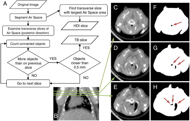
Automated detection of the axial extents of the ROI. (A) A flowchart illustrating the algorithm for finding the transverse slice locations for the posterior (HDI) and anterior (TB) ends of the chest space ROI. At the HDI slice, the air space area is at its maximum in the transverse plane. The TB slice is determined by examining transverse 2D slices of the air space image starting from the anterior end of the lung. C to E show transverse cross sections of the micro-CT data at different slice locations that are indicated on a coronal cross section (B). The corresponding images of segmented lung air space (black) within the body mask (white) are shown in F to H. Connected air space objects on each slice are identified (arrows on F–H). At first, the trachea appears as the only object (F). If a new object appears (G), but the objects are further than 0.5 mm apart from each other, the algorithm continues. At the TB slice (H), the trachea object splits into two closely spaced objects (left and right bronchi).

TB detection algorithm

The transverse slice location for the TB defining the anterior end of the ROI is determined as follows: First, a body mask of the mouse is created by intensity thresholding the image (vivaCT 40: − 470 HU, eXplore CT120: − 400 to 2000 HU), finding the largest three-dimensional (3D) object of six-connected voxels, and filling eight-connected holes on 2D transverse slices. The lung air space (including alveolar tissue) is segmented by intensity thresholding (upper threshold, vivaCT 40: − 470 HU, eXplore CT120: − 400 HU) the image, where the body mask is applied to exclude the air outside the mouse. Starting from the anterior end of the binary lung air space image, going in the posterior direction, transverse 2D slices are examined by finding objects of eight-connected pixels of the air space. The trachea appears as the only connected object of the air space until the bifurcation is reached, where a new connected object appears. An additional rule applied to avoid false detection from other possible objects, such as a lobe of the lung, is that the two objects (left and right bronchi) have to be within 0.5 mm from each other at the TB slice. The procedure is illustrated in Figure 2.

HDI detection algorithm

At the posterior end of the lung, it is important to exclude the diaphragm from the ROI. The air space area is calculated on transverse 2D slices of the segmented lung air space images. Starting from the slice at the posterior end of the lung, going in the anterior direction, the air space area increases rapidly and reaches a maximum when the diaphragm disappears. From that point forward, the tapering of the lung and increasing heart area cause the air space area to decrease. This maximum in air space area defines the HDI, which is chosen as the posterior end of the ROI.

Segmentation of the chest space

The rib cage is segmented by first applying a lower intensity threshold (vivaCT 40: 840 HU, eXplore CT120: 175 HU) and a morphologic close (vivaCT 40: 5 × 5 × 5, eXplore CT120:3 × 3 × 3) operation to the original image to segment the bone and then combining six-connected voxels into 3D objects. The largest connected object is kept and it includes the ribs, vertebrae, and sternum but excludes the scapula and the front limb bones. On each transverse 2D slice of the rib cage image between the TB and the HDI, connected pixels are combined into objects and the innermost (closest to the body mask centroid) points of these objects are used for creating a mask of the chest space. The points are first ordered clockwise by their direction from the centroid of the body mask. If any two points form a low angle of less than 12° between them (measured from the body centroid) and are located on the dorsal side of the mouse, the further one is removed from the point list. The distant points that meet these criteria are typically from further sections of the vertebrae and could cause undesirable effects in the following step if not removed (Figure 3). The remaining points are then connected by fitting a smooth closed curve trace (spline) to them. The area bounded by the trace is morphologically filled to create a binary mask of the chest space. The resulting 3D chest space ROI is axially smoothed by applying a 1 × 1 × 5 median filter and a 1D gap-filling operation in the axial direction.

Figure 3.

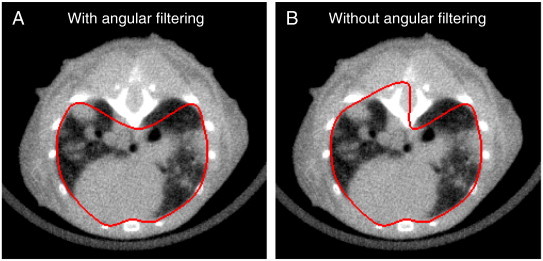
Illustration of the automated chest space segmentation. The innermost points of the bones on transverse slices are first ordered by the angle they form from the body center. Measured from the body center, if any two points form a low angle of less than 12° between them and are located on the dorsal side, the further one is removed from the point list. The remaining points are then connected by a smooth closed spline (shown in red) that is filled to create the chest space mask (A). If no angular filtering was applied to the points, the mask would be too inclusive in this case (B).

The soft tissue is segmented by employing the same thresholding and morphologic filtering procedures as described under the Tracing Analysis section, and the tissue volume is calculated within the automatically detected chest space ROI.

Estimating the heart size

The heart is indistinguishable from the tumor tissue by image intensities. Moreover, tumors can be attached to the heart without a visible boundary, making it very difficult to segment the entire heart in the images automatically and robustly. Therefore, our approach is to get an estimate of the shortest principal axis length of the heart and employ this in a model to estimate the total heart volume. The estimate of shortest principal axis does not require a well-defined boundary encompassing the entire heart.

The chest space mask from the previous step is dilated by 20 voxels to insure that the heart would be entirely enclosed in it. The segmented soft tissue image is morphologically closed (3 × 3 × 3) and masked with the dilated chest space mask, and the heart radius is estimated by fitting the largest possible sphere within the masked soft tissue. The sphere is bounded by the ribs and sternum on the ventral side and the lung air space on the dorsal side. Even when tumors are connected to the heart, the bronchi typically remain around the heart to limit the boundaries. Furthermore, to limit the effect of a possible overestimation of the heart size due to significant tumor growth, an upper limit of 3.6 mm is imposed on the heart radius. This value was chosen as r_m + 2 * SD, where the mean radius (r_m = 3.2 mm) and the standard deviation (SD = 0.2 mm) of the radius were measured in non–tumor-bearing mice in a separate study.

The heart is modeled as a skewed ellipsoid with the principal axes lengths a = 2r, b = 2.6r, and c = 3.2r, where r is the heart radius estimated by the algorithm. The volume of the heart included in the ROI is calculated with the equation below as the volume (V) of an ellipsoidal cap, the height of which is the axial ROI length (L):

$$\mathrm{Ellipsoidal}\mathrm{cap}\mathrm{volume}:V=\frac{\pi ab}{3c^2}{L}^2\left(3c-L\right)\text{.}$$ (1)

Figure 4 illustrates the skewed ellipsoid with the directions of its two longest principle axes and its relation to the axial extents of the ROI (TB and HDI). Finally, the ellipsoidal cap volume is subtracted from the tissue volume in the rib cage to calculate the automated tissue volume (ATV).

Figure 4.

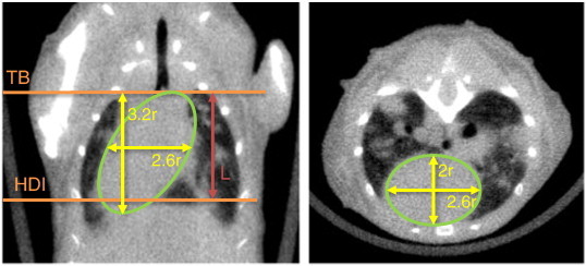
Estimating the heart volume. A large portion of the heart is included within the automatically defined ROI. The volume of the included heart is estimated by modeling it as a skewed ellipsoidal cap of length L between the TB and HDI. The dimensions of the ellipsoid are 3.2r, 2.6r, and 2r, where r is the radius of the maximum sphere that fits inside the heart.

The validity of the automated heart size estimates was confirmed by manually tracing the hearts in the validation study. The heart boundaries were traced on six to eight transverse slices between the identified TB and HDI slices and propagated between the traces. The traced heart volumes were compared against the ellipsoidal cap volumes calculated in the previous step.

Quality control and manual corrections

If the algorithm fails in determination of the TB or HDI or in segmentation of the rib cage, it is important to detect the failure and enable manual correction in a way that is compatible with the automated results from other scans. The analysis program creates a 3D surface rendering from the image that shows the ROI in relation to the skeleton as shown in Figure 5. These renderings can be quickly reviewed to determine if the ROI is appropriately located within the rib cage. The analysis software also includes an automatic range checking for the axial length of the ROI. If the length falls outside the normal range (6-10 mm), the ROI is manually examined for possible failure in the TB or HDI detection. In case of failed TB or HDI detection, the user manually indicates the correct TB and HDI slice locations, and the rib cage is segmented by the algorithm. If the rib cage mask is incorrectly segmented, the user traces the inside of the rib cage on six to eight evenly spaced slices between the TB and HDI, and the ROI is completed by propagating between the traces.

Figure 5.

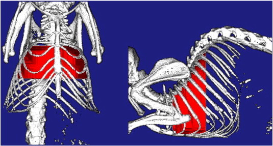
Automatically defined ROI for quantifying the lung tumor burden. Surface rendering of the ROI (red) defined by the automated method is shown in relation to the mouse skeleton. These renderings are automatically generated by the analysis program and used for a visual check of the ROI as part of the quality control procedure.

Statistical analysis

All data values presented are mean ± SD, and the error bars on the graphs represent standard error of mean (SEM). All statistical analyses were performed with JMP 11 software (SAS, Cary, NC). Pearson linear correlation coefficient (r) was calculated to compare ATV with the manual tumor burden metrics (SCP and TVV). Since SCP is a cross-sectional tumor area metric while ATV is a 3D metric, the Spearman rank correlation coefficient (r_s) was also calculated. The change in tumor burden metrics from baseline (∆SCP, ∆TVV, and ∆ATV) was used as a metric of treatment efficacy, and the treatment groups were compared against the control group using the Dunnett test, with P values less than .05 considered significant.

Results

Validation Study

In the validation study, mice were scanned on the micro-CT pre-treatment and 4 weeks after start of the treatment. Tumor burden was evaluated from the image data by the automated method and compared to the two manual analysis methods: cross-product analysis and tracing analysis, which were performed by a single reader (H.B.-R.). For the automated analysis, 12 of the 72 data sets required a manual correction to indicate either the anterior or the posterior end slice, or the outline of the rib cage. Corrections were done by a single reader (K.H.B.). A representative image of the ROI defined by the automated method in the validation study is shown in Figure 5.

The mean values for the different tumor burden metrics of all mice at pre-treatment and post-treatment time points were, respectively, ATV: 269±145 mm³, 334±172 mm³; TVV: 211±164 mm³, 286±192 mm³; SCP: 39±29 mm², 51±33 mm². Scatterplots of ATV versus SCP and TVV and of ∆ATV versus ∆SCP and ∆TVV are shown in Figure 6. The ATV was well correlated with both SCP (r = 0.88, r_s = 0.81, P < .0001) and TVV (r = 0.93, P < .0001). The change in ATV from baseline (∆ATV) was also well correlated with both ∆SCP (r = 0.83, r_s = 0.74, P < .0001) and ∆TVV (r = 0.90, P < .0001). From the scatterplot between ATV and SCP (Figure 6A), it can be seen that in the absence of visible tumors (SCP = 0 mm²), ATV had a bias value of approximately 100 mm³ from non-tumor soft tissues that are included in the ROI. TVV also has a bias volume, which is lower (approximately 50 mm³) due to the differences in the included regions between the automated and tracing methods, such as the mediastinum and soft tissue at the anterior end of the lung that were excluded in the tracing analysis for TVV.

Figure 6.

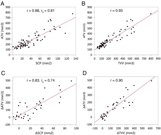
Comparison of the ATV to manual tumor burden metrics, SCP and TVV, of all scans in the validation study. ATV showed good correlation to both SCP (A) and TVV (B). The change in ATV from baseline (∆ATV) was also well correlated with ∆SCP (C) and ∆TVV (D). P < .0001 for all correlations.

The automated estimates of heart volumes correlated well with the manual estimates (r = 0.84, P < .0001; Figure 7) and had similar mean values (automated: 256 ± 39 mm³, manual: 254 ± 33 mm³). The average minimum heart radius estimated by the algorithm was 3.2 ± 0.2 mm. A small but statistically significant reduction in the heart radius estimate from pre-treatment to post-treatment was observed in the anti-VEGF + chemo group (− 3%, P < .05, paired t test) but not in the other groups.

Figure 7.

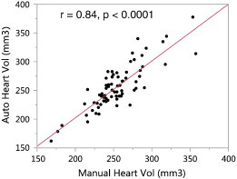
Validation of the automated heart volume estimates. Heart volumes estimated by the automated method (on y-axis) were validated against manual tracing (on x-axis). The volume estimates showed similar values and good correlation.

A correlative relationship was observed between the chest space volume and tumor burden, evidenced by a positive correlation between the volume of the automatically generated ROI and SCP (r = 0.79, P < .0001; Figure 8A). The change in the ROI volume in individual animals during the study was also correlated with the change in SCP (r = 0.74, P < .0001; Figure 8B). The air space volume within the ROI, calculated by subtracting the segmented tissue volume from the ROI volume, did not correlate with the tumor burden (r = 0.23, P > .05; Figure 8C). This shows that the chest space volume in the mice got larger as their tumor burden increased, while the air space volume was not affected.

Figure 8.

Evidence of chest space volume increase due to tumor growth. (A) The volume of the automatically generated ROI (on the y-axis) was larger at higher tumor burden (SCP on the x-axis). (B) The change in the ROI volume from pre-treatment to post-treatment in individual mice was also correlated with the change in tumor burden. However, the air space volume within the ROI did not depend on the tumor burden (C). This shows that the chest space volume in the mice increased with increasing tumor burden. The mice likely compensate for the space taken up by the tumors by increasing the chest space to maintain adequate functional lung capacity and ventilation.

All tumor burden metrics showed significant reduction in tumor growth in both the anti-VEGF group (∆SCP: − 90%, P < .001, ΔTVV: − 69%, P < .01, ∆ATV: − 68%, P < .01) and the anti-VEGF + chemo group (∆SCP: − 87%, ΔTVV: − 94%, ∆ATV: − 99%, P < .001 for all) compared to the control group (Figure 9).

Figure 9.

Treatment efficacy in the validation study. Treatment effect on tumor growth was evaluated by comparing change (Δ) in the tumor burden metrics (A) ΔSCP, (B) ΔTVV, and (C) ΔATV, from pre-treatment to post-treatment imaging (4 weeks later), between groups. Points show individual animals, the horizontal lines are the group means, and the error bars are SEM. Treatment groups were compared to control by Dunnett test: *P < .01, **P < .001.

High-Throughput Serial Study

In the high-throughput study, mice were imaged every 2 weeks for 8 weeks from the start of treatment on week 16 post-infection. All mice (n = 9 per group) were alive on weeks 16 and 18. At the following time points, the numbers of surviving animals for each group were (control, chemo, anti-VEGF, anti-VEGF + chemo, respectively) eight, nine, nine, and nine for week 20, six, three, eight, and nine for week 22, and four, two, seven, and nine for week 24.

Tumor burden was evaluated with the automated method as well as the manual tracing method for comparison. The automated ROI’s were corrected for 9 of the 155 data sets by a single reader (K.H.B.). Mice were randomly assigned to two readers (J.E.L. and R.M.) for tracing analysis, and all time points for each mouse were read by the same person. Good correlations were observed between ATV and TVV (r = 0.90, P < .0001; Figure 10A) and between ∆ATV and ∆TVV (r = 0.85, P < .0001; Figure 10B), similar to the validation study. Figure 11 shows the time courses (mean ± SEM) of ∆ATV and ∆TVV for each group. The control group and chemo group were not plotted past week 20 as they were missing significant numbers of mice compared to the earlier time points due to high attrition rates for these two groups. Starting from week 18, both ∆ATV and ∆TVV were significantly reduced in anti-VEGF group (∆ATV: P < .005, ∆TVV: P < .05 for all time points) and anti-VEGF + chemo group (∆ATV: P < .0001, ∆TVV: P < .005 for all time points), and ∆ATV was significantly reduced for the chemo group (P < .05 for all time points) when compared to control (Dunnett test). Similarly to the finding in the validation study, the heart radius estimate in the anti-VEGF + chemo group was reduced from baseline at all four post-treatment time points (− 7%, − 8%, − 7%, − 4%, P < .005, paired t test).

Figure 10.

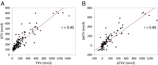
Comparison of tissue volume metrics in the high-throughput serial study. (A) ΔATV and manually traced ΔTVV values and (B) change from baseline, ∆ATV and ∆TVV. P < .0001 for both correlations.

Figure 11.

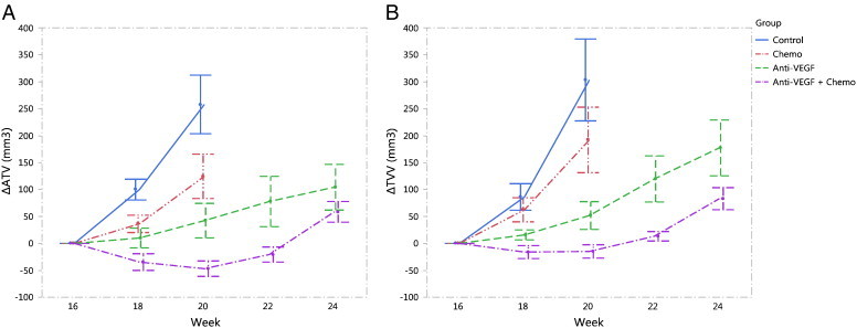
Treatment efficacy in the high-throughput serial study. Treatment started on week 16 post-infection. The change in tissue volume measured by both (A) automated method and (B) manual tracing method showed significant treatment effect (P < .05, Dunnett test) by both anti-VEGF and anti-VEGF + chemo therapies starting on the first post-treatment imaging time point (week 18 post-infection). After week 20, the control and chemo groups are not shown on the graphs due to losing significant numbers of the mice. Data points show group mean ± SEM.

Discussion

In this manuscript, a novel automated image analysis method for estimating the lung tumor burden in an NSCLC GEMM imaged by in vivo micro-CT has been introduced. The general principle of using segmented soft tissue within an ROI in the lung is similar to the method proposed by Haines et al. [12], but instead of manually contouring the ROI, the algorithm presented here automatically finds fixed anatomic landmarks (TB, HDI, and rib cage) that define the ROI boundaries. The algorithm also estimates the heart size and subtracts it from the tissue volume. The obvious advantage of automating the analysis is saving time, but perhaps even more importantly, it makes the analysis objective and reproducible. The algorithm also does not require the user to be able to differentiate tumors from other soft tissue, which becomes challenging when large tumors grow attached to the heart and the diaphragm. This situation can also cause the automated method to overestimate the heart radius, but the effect of this is limited by imposing a maximum limit for the radius. In these cases, the tumor burden is large and the error from not having an accurate heart size estimate becomes relatively small. Conversely, at low tumor burden when accurate heart size estimates are more important for reducing variability, the algorithm is also more likely to be accurate since there is less chance of a large tumor being attached to the heart.

The method was validated by comparison against two previously validated manual analysis techniques: the cross-product method [3] and the tracing method, which was based on a description by Haines et al. [12]. Unidimensional or bidimensional measurements of tumors, similar to the cross-product method used here, are typically used in clinical setting to evaluate tumor progression [23,24]. The cross-product analysis is particularly challenging when tumors start connecting to each other and are difficult to tell apart. Measuring previously separated tumors as one contiguous tumor may lead to underestimating the tumor burden. The volumetric methods are not hindered by this but are less sensitive at detecting a single small nodule in the lung due to variability in the other included soft tissues. The comparison of tumor volumes with the SCP is somewhat complicated by their non-linear relationship. Nevertheless, the tumor burden measured by all three methods correlated well and showed similar therapeutic responses.

The automated method was also applied to a study that was performed on a high-throughput micro-CT scanner where four mice can be simultaneously scanned in 5 minutes. This allows completing the scanning and analysis of more than 100 mice per day by a single person. A good correlation between automated and manual tissue volumes was observed in this study as well, and the automated method showed a similar treatment effect on tumor growth by anti-VEGF therapy alone and in combination with chemotherapy, as was also observed in the validation study. A small reduction in tumor growth was also observed by chemotherapy alone, which could be a result of using a more aggressive chemotherapy regimen in this study.

In tumor-bearing mice, the lung morphology changes as the disease progresses. An increase in the chest space volume was observed with increasing tumor burden, as has been previously reported by Haines et al. [12]. This volume increase is likely due to a compensatory response to maintain adequate functional air space and ventilation as the lung becomes occupied by the growing tumors. To include the same lung regions in the ROI, it is important to define the ROI by anatomic landmarks that relate to the lung itself and not only the skeletal structures around it.

In both studies, a reduction was observed in the minimum heart radius estimated by the algorithm in mice treated with a combination of anti-VEGF and chemotherapy. Further investigation would be required to determine the cause of the reduction and whether it relates to a change in the heart muscle tissue volume, blood volume, or some physiological alteration in diastolic volume that results in apparent size change in the heart. No significant changes in heart size were observed in the other groups. This shows the importance of estimating the heart size, not only to reduce variability but also to avoid biasing results by a potential drug effect on the heart.

In the presented studies, a manual correction to accurately identify the bounding anatomic structures (rib cage, TB, or HDI) was needed in less than 10% of all scans (validation study: 16.7%, high-throughput study: 5.8%). The correction typically takes less than 5 minutes per scan to complete. Errors in the rib cage segmentation can result from image artifacts caused by a shift in the mouse position during the scan but not by regular breathing motion. The TB or HDI detection can fail due to heavy tumor burden obstructing one of the bronchi at the TB or filling the area around the HDI. These situations can be identified and corrected by the user following the steps outlined in the Quality control and manual corrections section. Even when manual input is required, the method limits the possible variability from reader interpretation since the bounding anatomic structures are relatively unambiguous to identify and the reader is typically not required to distinguish tumor tissue from other identical appearing soft tissue. Consequently, the intra-reader and inter-reader variability and manual versus automated variability are expected to be small, although they were not evaluated in this study. In rare situations where the tumor burden is so severe that even the reader cannot determine the HDI, it is recommended to match the number of included slices (TB to HDI) between the baseline and later scans so that approximately the same regions in the lung are included.

The presented automated method does not address a potential heterogeneity of treatment response in tumors, which would require identification and measurement of individual tumors at different time points. Another limitation of the method is that the portion of the lung posterior to the HDI is excluded from the analysis and any tumors located in this region would therefore not contribute to the tissue volume. The excluded lung region is approximately 15% of the entire chest space volume and typically contains less than 25% of the tumors. As shown by the correlation and similar treatment responses between ATV and TVV, this omission did not significantly affect the results, but it may be a concern in a model that exhibits a low tumor burden. Improving the inclusion would require detecting the curved surface of the diaphragm, which can vary in shape and angle.

In conclusion, a novel automated analysis method was developed for quantifying the tumor burden from micro-CT images in an aggressive K-ras–driven GEMM of NSCLC where tumors can invade significant portions of the lung. The method should be readily applicable to other orthotopic mouse lung tumor models as well. The rapid and robust nature of this analysis method, combined with high-throughput micro-CT scanning, can provide a valuable tool in preclinical drug research for screening and randomizing animals into treatment groups as well as evaluating treatment efficacy non-invasively in GEMMs of lung cancer.

References

- 1.Ferlay J., Soerjomataram I., Dikshit R., Eser S., Mathers C., Rebelo M., Parkin D.M., Forman D., Bray F. Cancer incidence and mortality worldwide: sources, methods and major patterns in GLOBOCAN 2012. Int J Cancer. 2015;136:E359–E386. doi: 10.1002/ijc.29210. [DOI] [PubMed] [Google Scholar]
- 2.Siegel R., Naishadham D., Jemal A. Cancer statistics, 2013. CA Cancer J Clin. 2013;63:11–30. doi: 10.3322/caac.21166. [DOI] [PubMed] [Google Scholar]
- 3.Singh M., Lima A., Molina R., Hamilton P., Clermont A.C., Devasthali V., Thompson J.D., Cheng J.H., Bou Reslan H., Ho C.C. Assessing therapeutic responses in Kras mutant cancers using genetically engineered mouse models. Nat Biotechnol. 2010;28:585–593. doi: 10.1038/nbt.1640. [DOI] [PubMed] [Google Scholar]
- 4.Jackson E.L., Olive K.P., Tuveson D.A., Bronson R., Crowley D., Brown M., Jacks T. The differential effects of mutant p53 alleles on advanced murine lung cancer. Cancer Res. 2005;65:10280–10288. doi: 10.1158/0008-5472.CAN-05-2193. [DOI] [PubMed] [Google Scholar]
- 5.Van Dyke T., Jacks T. Cancer modeling in the modern era: progress and challenges. Cell. 2002;108:135–144. doi: 10.1016/s0092-8674(02)00621-9. [DOI] [PubMed] [Google Scholar]
- 6.Junttila M.R., de Sauvage F.J. Influence of tumour micro-environment heterogeneity on therapeutic response. Nature. 2013;501:346–354. doi: 10.1038/nature12626. [DOI] [PubMed] [Google Scholar]
- 7.Aberle D.R., Adams A.M., Berg C.D., Black W.C., Clapp J.D., Fagerstrom R.M., Gareen I.F., Gatsonis C., Marcus P.M., Sicks J.D. Reduced lung-cancer mortality with low-dose computed tomographic screening. N Engl J Med. 2011;365:395–409. doi: 10.1056/NEJMoa1102873. [DOI] [PMC free article] [PubMed] [Google Scholar]
- 8.Manser R., Lethaby A., Irving L.B., Stone C., Byrnes G., Abramson M.J., Campbell D. Screening for lung cancer. Cochrane Database Syst Rev. 2013;6:CD001991. [Google Scholar]
- 9.De Clerck N.M., Meurrens K., Weiler H., Van Dyck D., Van Houtte G., Terpstra P., Postnov A.A. High-resolution X-ray microtomography for the detection of lung tumors in living mice. Neoplasia. 2004;6:374–379. doi: 10.1593/neo.03481. [DOI] [PMC free article] [PubMed] [Google Scholar]
- 10.Cavanaugh D., Johnson E., Price R.E., Kurie J., Travis E.L., Cody D.D. In vivo respiratory-gated micro-CT imaging in small-animal oncology models. Mol Imaging. 2004;3:55–62. doi: 10.1162/15353500200403184. [DOI] [PubMed] [Google Scholar]
- 11.Cody D.D., Nelson C.L., Bradley W.M., Wislez M., Juroske D., Price R.E., Zhou X., Bekele B.N., Kurie J.M. Murine lung tumor measurement using respiratory-gated micro-computed tomography. Investig Radiol. 2005;40:263–269. doi: 10.1097/01.rli.0000160070.67270.05. [DOI] [PubMed] [Google Scholar]
- 12.Haines B.B., Bettano K.A., Chenard M., Sevilla R.S., Ware C., Angagaw M.H., Winkelmann C.T., Tong C., Reilly J.F., Sur C. A quantitative volumetric micro-computed tomography method to analyze lung tumors in genetically engineered mouse models. Neoplasia. 2009;11:39–47. doi: 10.1593/neo.81030. [DOI] [PMC free article] [PubMed] [Google Scholar]
- 13.Fushiki H., Kanoh-Azuma T., Katoh M., Kawabata K., Jiang J., Tsuchiya N., Satow A., Tamai Y., Hayakawa Y. Quantification of mouse pulmonary cancer models by microcomputed tomography imaging. Cancer Sci. 2009;100:1544–1549. doi: 10.1111/j.1349-7006.2009.01199.x. [DOI] [PMC free article] [PubMed] [Google Scholar]
- 14.Kirsch D.G., Grimm J., Guimaraes A.R., Wojtkiewicz G.R., Perez B.A., Santiago P.M., Anthony N.K., Forbes T., Doppke K., Weissleder R. Imaging primary lung cancers in mice to study radiation biology. Int J Radiat Oncol Biol Phys. 2010;76:973–977. doi: 10.1016/j.ijrobp.2009.11.038. [DOI] [PMC free article] [PubMed] [Google Scholar]
- 15.Singh M., Couto S.S., Forrest W.F., Lima A., Cheng J.H., Molina R., Long J.E., Hamilton P., McNutt A., Kasman I. Anti-VEGF antibody therapy does not promote metastasis in genetically engineered mouse tumour models. J Pathol. 2012;227:417–430. doi: 10.1002/path.4053. [DOI] [PubMed] [Google Scholar]
- 16.Namati E., Thiesse J., Sieren J.C., Ross A., Hoffman E.A., McLennan G. Longitudinal assessment of lung cancer progression in the mouse using in vivo micro-CT imaging. Med Phys. 2010;37:4793–4805. doi: 10.1118/1.3476454. [DOI] [PMC free article] [PubMed] [Google Scholar]
- 17.Rodt T., von Falck C., Dettmer S., Hueper K., Halter R., Hoy L., Luepke M., Borlak J., Wacker F. Lung tumour growth kinetics in SPC-c-Raf-1-BB transgenic mice assessed by longitudinal in-vivo micro-CT quantification. J Exp Clin Cancer Res. 2012;31:15. doi: 10.1186/1756-9966-31-15. [DOI] [PMC free article] [PubMed] [Google Scholar]
- 18.Li M., Jirapatnakul A., Biancardi A., Riccio M.L., Weiss R.S., Reeves A.P. Growth pattern analysis of murine lung neoplasms by advanced semi-automated quantification of micro-CT images. PLoS One. 2013;8:e83806. doi: 10.1371/journal.pone.0083806. [DOI] [PMC free article] [PubMed] [Google Scholar]
- 19.Rudyanto R.D., Bastarrika G., de Biurrun G., Agorreta J., Montuenga L.M., Ortiz-de-Solorzano C., Munoz-Barrutia A. Individual nodule tracking in micro-CT images of a longitudinal lung cancer mouse model. Med Image Anal. 2013;17:1095–1105. doi: 10.1016/j.media.2013.07.002. [DOI] [PubMed] [Google Scholar]
- 20.Sande E.P., Martinsen A.C., Hole E.O., Olerud H.M. Interphantom and interscanner variations for Hounsfield units–establishment of reference values for HU in a commercial QA phantom. Phys Med Biol. 2010;55:5123–5135. doi: 10.1088/0031-9155/55/17/015. [DOI] [PubMed] [Google Scholar]
- 21.http://www.scanco.ch/en/support/faq-general.html
- 22.Jain A. Prentice-Hall; Englewood Cliffs, NJ: 1989. Fundamentals of digital image processing. [Google Scholar]
- 23.James K., Eisenhauer E., Christian M., Terenziani M., Vena D., Muldal A., Therasse P. Measuring response in solid tumors: unidimensional versus bidimensional measurement. J Natl Cancer Inst. 1999;91:523–528. doi: 10.1093/jnci/91.6.523. [DOI] [PubMed] [Google Scholar]
- 24.Eisenhauer E.A., Therasse P., Bogaerts J., Schwartz L.H., Sargent D., Ford R., Dancey J., Arbuck S., Gwyther S., Mooney M. New response evaluation criteria in solid tumours: revised RECIST guideline (version 1.1) Eur J Cancer. 2009;45:228–247. doi: 10.1016/j.ejca.2008.10.026. [DOI] [PubMed] [Google Scholar]