Correction for the T1 Effect Incorporating Flip Angle Estimated by Kalman Filter in Cardiac-Gated Functional MRI

Abstract

Purpose

To develop an improved and generalized technique for correcting T1-related signal fluctuations (T1 effect) in cardiac-gated functional magnetie resonance imaging (fMRI) data with flip angle estimation.

Theory and Methods

Spatial maps of flip angle and T1 are jointly estimated from cardiac-gated time series using a Kalman filter. These maps are subsequently used for removing the T1 effect in the presence of B1 inhomogeneity. The new technique was compared with a prior technique that uses T1 only while assuming a homogeneous flip angle of 90°. The robustness of the new technique is demonstrated with simulated and experimental data.

Results

Simulation results revealed that the new method led to increased temporal signal-to-noise ratio across a large range of flip angles, T1s, and stimulus onset asynchrony means compared to the T1 only approach. With the experimental data, the new approach resulted in higher average gray matter temporal signal-to-noise ratio of seven subjects (84 vs. 48). The new approach also led to a higher statistical score of activation in the lateral geniculate nucleus (P < 0.002).

Conclusion

The new technique is able to remove the T1 effect robustly and is a promising tool for improving the ability to map activation in fMRI, especially in subcortical regions.

INTRODUCTION

The central challenge in functional magnetic resonance imaging (fMRI) is the detection of relatively small activity-induced signal changes (<5%) in the presence of various other signal fluctuations. Heartbeat-related pulsation of blood flow and cerebrospinal fluid (CSF) due to cardiovascular processes causes artifacts near ventricles, sulci, and large vessels (1,2). Large vessel pulsatility may cause tissue movement and produce an influx of unsaturated spins into the slice of interest (1). These changes can reduce the fMRI’s ability to detect hemodynamic changes related to neural activity. Retrospective correction (2,3) has been commonly used to reduce physiological fluctuations. However, the motion of the brain itself, as well as pulsatile flow of CSF and large vessels, makes retrospective correction of cardiac noise difficult, especially in subcortical regions such as brainstem and thalamus.

To overcome this problem, cardiac-gated acquisition has been introduced as a means to freeze pulsation-induced brain movement (4). The primary difficulty with this strategy lies in the pulse repetition time (TR) inconsistency due to the variation of the cardiac cycle. This TR variability introduces T1-related signal fluctuations (denoted “T1 effect”, ~7% with a TR that has a 10% variation around 1 s, T1 = 1600 ms, and flip angle = 90° for gray matter), which may overwhelm the BOLD signal change (< 5%). A passive approach to avoid this variation is to use a TR long enough (e.g. > 5× T1) to reach nearly full T1 relaxation in each measurement (5). However, such an approach inevitably sacrifices temporal resolution and data acquisition efficiency. A processing technique previously introduced for correcting the T1 effect (4,6) is effective but is only valid at a flip angle of 90°. B1 inhomogeneity can often cause significant variation in flip angle, e.g., 65–105° over the entire brain for a nominal flip angle of 90° at 3T (7,8). In the presence of such spatial inhomogeneity, the existing technique is not effective over the entire imaged volume even for a nominal flip angle of 90°. Moreover, when a nominal flip angle less than 90° such as the Ernst angle is used, the existing correction technique is inappropriate.

In this article, we describe an improved and generalized technique for correcting the T1 effect in cardiac-gated fMRI data incorporating the flip angle as estimated from the fMRI dataset itself. Using an unscented Kalman filter (9), spatial maps of flip angle and T1 are estimated simultaneously from the cardiac-gated time series. These maps are subsequently used for removing the T1 effect in the fMRI data. The robustness of this new approach is demonstrated with simulated and experimental data.

THEORY

MR Signal Model

In a gated fMRI run, the longitudinal magnetization before the k^th RF pulse is applied, $M_{z,k}^{-}$, is described in Ref. (10):

$$M_{z,k}^{-}=M_{z,k-1}^{-}\text{cos}\mathrm{\alpha }{e}^{-\frac{\mathrm{T}{\mathrm{R}}_k}{\mathrm{T}1}}+M_0(1-e^{-\frac{\mathrm{T}{\mathrm{R}}_k}{\mathrm{T}1}})$$ [1]

where M₀ is the equilibrium magnetization, TR is the repetition time, α is the nominal flip angle, and k denotes the time point. The transverse magnetization M_xy,k obtained by multiplying sin α to both sides of Eq. 1, noting that $M_{xy,k}=M_{z,k}^{-}\text{sin}\mathrm{\alpha }$, is

$$M_{xy,k}=M_{xy,k-1}\text{cos}\mathrm{\alpha }{e}^{-\frac{\mathrm{T}{\mathrm{R}}_k}{\mathrm{T}1}}+M_0\text{sin}\mathrm{\alpha }(1-e^{-\frac{\mathrm{T}{\mathrm{R}}_k}{\mathrm{T}1}}).$$ [2]

The MR signal for the k^th time point, $m_k\triangleq M_{xy,k}{e}^{-\frac{\mathrm{T}\mathrm{E}}{\mathrm{T}{2}_k^{*}}}$ becomes

$$m_k=M_{xy,k-1}{e}^{-\frac{\mathrm{T}\mathrm{E}}{\mathrm{T}{2}_k^{*}}}\text{cos}\mathrm{\alpha }{e}^{-\frac{\mathrm{T}{\mathrm{R}}_k}{\mathrm{T}1}}+M_0\text{sin}\mathrm{\alpha }{e}^{-\frac{\mathrm{T}\mathrm{E}}{\mathrm{T}{2}_k^{*}}}(1-e^{-\frac{\mathrm{T}{\mathrm{R}}_k}{\mathrm{T}1}})$$ [3]

$$=m_{k-1}{e}^{(\frac{\mathrm{T}\mathrm{E}}{\mathrm{T}{2}_{k-1}^{*}}-\frac{\mathrm{T}\mathrm{E}}{\mathrm{T}{2}_k^{*}})}\text{cos}\mathrm{\alpha }{e}^{-\frac{\mathrm{T}{\mathrm{R}}_k}{\mathrm{T}1}}+M_0\text{sin}\mathrm{\alpha }{e}^{-\frac{\mathrm{T}\mathrm{E}}{\mathrm{T}{2}_k^{*}}}(1-e^{-\frac{\mathrm{T}{\mathrm{R}}_k}{\mathrm{T}1}}).$$ [4]

In the absence of noise, the T2* term $e^{-\frac{\mathrm{T}\mathrm{E}}{\mathrm{T}{2}_k^{*}}}$ varies only as a result of the BOLD contrast. Because the BOLD signal varies gradually (11) and increases of T2* following the onset of neuronal stimulation are accompanied by decreases back to baseline, i.e., the mean of $\frac{\mathrm{T}\mathrm{E}}{\mathrm{T}{2}_{k-1}^{*}}-\frac{\mathrm{T}\mathrm{E}}{\mathrm{T}{2}_k^{*}}$ is nearly 0, we assume $e^{(\frac{\mathrm{T}\mathrm{E}}{\mathrm{T}{2}_{k-1}^{*}}-\frac{\mathrm{T}\mathrm{E}}{\mathrm{T}{2}_k^{*}})}$ to be 1 for the purpose of estimating the flip angle and T1. With this approximation, the MR signal is given by

$$m_k=m_{k-1}\text{cos}\mathrm{\alpha }{e}^{-\frac{\mathrm{T}{\mathrm{R}}_k}{\mathrm{T}1}}+M_0\text{sin}\mathrm{\alpha }{e}^{-\frac{\mathrm{T}\mathrm{E}}{\mathrm{T}{2}_k^{*}}}(1-e^{-\frac{\mathrm{T}{\mathrm{R}}_k}{\mathrm{T}1}}).$$ [5]

T1 Only Correction

For the special case of α being 90°, the MR signal given by Eq. 5 is simplified to

$$m_k=M_0{e}^{-\frac{\mathrm{T}\mathrm{E}}{\mathrm{T}{2}_k^{*}}}(1-e^{-\frac{\mathrm{T}{\mathrm{R}}_k}{\mathrm{T}1}}).$$ [6]

In conventional ungated acquisition (e.g., TR_k = 2 s), the T1-dependent signal term $1-e^{-\frac{\mathrm{T}{\mathrm{R}}_k}{\mathrm{T}1}}$ is constant, whereas the T2*-dependent signal term provides the signal contrast of interest. However, in cardiac-gated acquisition, MR signal is also modulated by the T1-dependent term due to the variation of the cardiac cycle. This T1 effect may overwhelm the T2* signal change. Correction techniques for this T1 effect were developed for the special case of α being 90° (4,6). With measurements using TRs of 20 s and 1 s, respectively, one can estimate the T1, assuming that a TR of 20 s allows full T1 signal recovery (6). With estimated $\widehat{\mathrm{T}1}$ and average TR, the correction is made using

$$m_{k,\text{cor}}=m_k\left[\frac{1-e^{-\mathrm{T}{\mathrm{R}}_{\text{avg}}/\widehat{\mathrm{T}1}}}{1-e^{-\mathrm{T}{\mathrm{R}}_k/\widehat{\mathrm{T}1}}}\right].$$ [7]

In the presence of spatial inhomogeneity of B1, this correction is not valid over the entire imaged volume even for the nominal flip angle of 90°.

T1 Correction with Flip Angle Estimation

In this article, we describe a generalized technique for correcting the T1 effect taking into account the actual flip angle. We first estimate the flip angle and the T1. An unscented Kalman filter, a recursive minimum mean square error estimator based on the optimal gaussian approximate Kalman filter framework (12), is used to simultaneously estimate the T1 and the flip angle from the fMRI time series. Kalman filters have been widely used for nonlinear estimation, including estimation of the state of a nonlinear dynamic system such as an fMRI time series (13). The basic framework for Kalman filtering involves the estimation of the state of a discrete-time dynamic system described in a state-space model,

$${\mathbf{S}}_k=f({\mathbf{S}}_{k-1},{\mathbf{v}}_k)$$ [8]

$$y_k=h({\mathbf{S}}_k,w_k),$$ [9]

where S_k represents the random state variable of the system and y_k is the measured signal. The state and measurement noises are given by v_k and w_k, respectively. The system dynamic models, f(·) and h(·), are assumed to be known. The Kalman filter involves the recursive estimation of the mean and covariance of the state and consists of two steps, prediction and updating (14):

$${\mathbf{Ŝ}}_k=(\text{prediction of}{\mathbf{S}}_k)+{\mathbf{K}}_k(y_k-(\text{prediction of}{y}_k))={\mathbf{Ŝ}}_k^{-}+{\mathbf{K}}_k(y_k-{ŷ}_k^{-})$$

$${\mathbf{P}}_{{\mathbf{S}}_k}={\mathbf{P}}_{{\mathbf{S}}_k}^{-}-{\mathbf{K}}_k{\mathbf{P}}_{{ỹ}_k}{\mathbf{K}}_k^T,$$ [10]

where K_k denotes the optimal Kalman gain, the optimal predictions of S_k and y_k are written as ${\mathbf{Ŝ}}_k^{-}$ and ${ŷ}_k^{-}$, respectively, and the covariance matrix is represented as P. The optimal terms in this recursion for a given system are expressed by

$${\mathbf{Ŝ}}_k^{-}=𝔼[f({\mathbf{S}}_{k-1},{\mathbf{v}}_k)]$$

$${ŷ}_k^{-}=𝔼[h({\mathbf{S}}_k^{-},w_k)]$$

$${\mathbf{K}}_k=𝔼[({\mathbf{S}}_k-{\mathbf{Ŝ}}_k^{-}){(y_k-{ŷ}_k^{-})}^T]𝔼{[(y_k-{ŷ}_k^{-}){(y_k-{ŷ}_k^{-})}^T]}^{-1}={\mathbf{P}}_{{\mathbf{S}}_k{ỹ}_k}{\mathbf{P}}_{{ỹ}_k}^{-1},$$ [11]

where ${\mathbf{Ŝ}}_k^{-}$ and ${ŷ}_k^{-}$ are the expectation values of the corresponding random variables and ỹ_k is the prediction error (or innovation, $y_k-{ŷ}_k^{-}$). The Kalman gain K_k is expressed as a function of the expected cross-covariance matrix of the state prediction error and the measurement prediction error as well as the expected autocorrelation matrix of the measurement prediction error. The optimal solution for the Kalman filter requires taking expectations of a nonlinear function of state variables, which can be approximated by an unscented transformation. The unscented transformation is a method to propagate the statistics of a random variable through nonlinear transformations, building on the principle that “it is easier to approximate probability distributions than it is to approximate an arbitrary nonlinear function or transformation (15).” Please refer to the Appendix for details on unscented transformation and unscented Kalman filter.

Now, we put the MR signal model given in Eq. 5 into the Kalman filter framework. The state random variable S_k consists of the flip angle, T1, T2* signal change, and MR signal at the k^th time point:

$${\mathbf{S}}_k=\left[\begin{array}{c}\hfill s_{k,1}\hfill \\ \hfill s_{k,2}\hfill \\ \hfill s_{k,3}\hfill \\ \hfill s_{k,4}\hfill \end{array}\right]=\left[\begin{array}{c}\hfill \mathrm{\alpha }\hfill \\ \hfill \mathrm{T}1\hfill \\ \hfill M_0\text{sin}\mathrm{\alpha }{e}^{-\frac{\mathrm{T}\mathrm{E}}{\mathrm{T}{2}_k^{*}}}\hfill \\ \hfill m_k\hfill \end{array}\right].$$ [12]

The MR signal time-series in Eq. 5 is represented as a state-space model, S_k = f (S_k−1, v_k):

$$s_{k,1}=s_{k-1,1}+v_{k,1}$$

$$s_{k,2}=s_{k-1,2}+v_{k,2}$$

$$s_{k,3}=s_{k-1,3}+v_{k,3}$$ [13]

$$s_{k,4}=s_{k-1,4}\text{cos}(s_{k,1})e^{-\frac{\mathrm{T}{\mathrm{R}}_k}{s_{k,2}}}+s_{k,3}(1-e^{-\frac{\mathrm{T}{\mathrm{R}}_k}{s_{k,2}}}),$$

where v_k = [v_k,1, v_k,2, v_k,3]^T is random gaussian state noise, v_k ~ N (0, P_vk). Note that T1 and the flip angle are modeled as random variables, allowing the propagation of model mismatch through nonlinear functions such as the exponential term and cosine term in the MR signal model. The measured signal y_k is described as:

$$y_k=h({\mathbf{S}}_k,w_k)=s_{k,4}+w_k$$ [14]

where w_k denotes random gaussian measurement noise, $w_k~(0,{\mathrm{\sigma }}_{w_k}^2)$.

Once the flip angle and the T1 are estimated as $\widehat{\mathrm{T}1}$ and α̂, the T2*-dependent signal term $M_0\text{sin}\mathrm{\alpha }{e}^{-\frac{\mathrm{T}\mathrm{E}}{\mathrm{T}{2}_k^{*}}}$ is estimated using two consecutive fMRI measurements from Eq. 5 by

$$M_0\text{sin}\mathrm{\alpha }{e}^{-\frac{\mathrm{T}\mathrm{E}}{\mathrm{T}{2}_k^{*}}}=\frac{m_k-m_{k-1}\text{cos}\hat{\mathrm{\alpha }}{e}^{-\mathrm{T}{\mathrm{R}}_k/\widehat{\mathrm{T}1}}}{1-e^{-\mathrm{T}{\mathrm{R}}_k/\widehat{\mathrm{T}1}}}.$$ [15]

Then, the corrected time series is generated using the general MR signal model given by Eq. 5 as follows:

$$m_{k,\text{cor}}=m_{k-1,\text{cor}}\text{cos}\hat{\mathrm{\alpha }}{e}^{-\frac{\mathrm{T}{\mathrm{R}}_{\text{avg}}}{\widehat{\mathrm{T}1}}}+M_0\text{sin}\mathrm{\alpha }{e}^{-\frac{\mathrm{T}\mathrm{E}}{\mathrm{T}{2}_k^{*}}}(1-e^{-\frac{\mathrm{T}{\mathrm{R}}_{\text{avg}}}{\widehat{\mathrm{T}1}}}).$$ [16]

METHODS

Simulation

Simulated cardiac-gated fMRI time series were generated from Eq. 4, which did not ignore the transient change of T2*, for a range of flip angles (60–110°) and T1s (800–2000 ms). TR variation was based on actual scan parameters from a representative subject. The T2* changes (3% variation around baseline) were included to simulate the block design BOLD signal change using the canonical hemodynamic response function based on experimental timing information described below. Noise was generated and added to achieve a temporal signal-to-noise ratio (tSNR) of 83 with a mixture of 70% white noise and 30% first-order autoregressive noise (16). Corrections for the T1 effect were performed using the “T1 only” and the “T1 & flip angle” methods. The performance of the correction was evaluated using tSNR, calculated by dividing the mean of a time series by its standard deviation. For simulation of event-related design, time series were generated from Eq. 4 incorporating hemodynamic response to a train of stimuli with jittered stimulus onset asynchrony (SOA) (17). The event-related simulations were performed for a range of mean SOA, from 2 to 20 s, and T1 of 1600 ms. In each case, the jittered SOA varied from 1 s to twice the mean.

Experimental Data

Physiological Recording

All physiological recording was performed using an integrated Siemens physiological monitoring Unit. The cardiac signal was monitored with a pulse oximeter placed on the subject’s finger, providing a delayed systolic signal as well as the oxygenation saturation level. Respiratory signal was monitored with a flexible pressure belt placed around the upper abdomen of subjects. The sampling frequency of all physiological recording was 50 Hz.

Data Acquisition

Seven healthy volunteers participated in the experimental study after giving informed consent in accordance with Emory University’s institutional review board. All MRI experiments were conducted on a 3T Siemens Tim Trio scanner (Siemens Medical Solutions, Malvern, PA) equipped with a 12-channel head coil. Anatomic images were acquired with a three-dimentional T1-weighted magnetization-prepared rapid gradient echo imaging sequence (field of view (FOV) = 256 × 256 × 176 mm³, resolution = 1 × 1 × 1 mm³, TR = 2250 ms, echo time (TE) = 2.52 ms, flip angle = 9°). Each subject subsequently underwent two randomly ordered fMRI scans, an ungated scan and a gated scan. The average heart rate was measured during the anatomical scan. All functional scans were acquired using a T2*-weighted echo-planar imaging sequence with the following parameters: 270-volumes, FOV = 220 × 220 mm², matrix = 110 × 110, eight ascending axial slices (thickness = 3 mm; gap = 0.6 mm), TE = 30 ms, generalized auto-calibrating partially parallel acquisition imaging with an acceleration factor of 2. For the gated scan, TR was determined by each subject’s heart rate. The average heart rate of each subject was used to determine the TR for the ungated scan to match the total scan time as well as the number of volumes. In addition, two volumes collected with the same parameters as the functional scans except with TRs of 1 s and 20 s were used to calculate T1 for the “T1 only” method.

Task Design

A central fixation cross was presented continuously and subjects were instructed to gaze at the cross during fMRI scans. Each fMRI scan started with 30 TRs of rest, followed by four sets of 30 TRs of visual stimulation, and 30 TRs of rest. An inverting half-filled checkerboard alternated between left and right hemifields at 8 Hz during the visual stimulation. Visual stimuli were generated by an LCD projector, back-projected onto a screen mounted at the rear of a scanner bore, and viewed through a mirror mounted on the head coil.

Data Analysis

For each subject, four types of time series were derived from the two scans: (1) an ungated scan; (2) a gated scan with no correction; (3) a gated scan with the “T1 only” correction; and (4) a gated scan with the “T1 & flip angle” correction. Analysis of Functional NeuroImages (AFNI, http://afni.nimh.nih.gov/afni) was used for most of the data analysis. In addition, The FMRIB Software Library (FSL, http://www.fmrib.ox.ac.uk/fsl/) was used for brain segmentation and registration. The “T1 & flip angle” correction was performed using Matlab (Math-Works, Natick, MA) routines with the ReBEL Matlab toolbox (http://choosh.csee.ogi.edu/rebel/) for the unscented Kalman filter. The first 10 volumes of each run were discarded to remove T1 saturation effects. Remaining volumes underwent motion correction, linear detrending, and spatial smoothing (full width at half maximum = 3 mm). Retrospective correction (2) was performed to reduce the respiration effect for all time-series and cardiac effects for ungated time series.

A multiple regression analysis was performed in the native space of each individual subject. Regressors representing the two visual stimulation conditions (left and right stimulus) and their temporal derivatives were used to derive subject level activation maps which reflect the contralateral response of the visual system. To compare temporal characteristics, the tSNR was calculated from the standard deviation of the residual time series produced by the regression analysis for each voxel. The regression coefficients were registered to standard space using FSL’s nonlinear image registration tool and fed into a one-sample t-test for deriving group level activation maps. The effect of different corrections on the activation was further examined by a regions of interest (ROI) analysis. Two ROIs were functionally defined; one in the lateral geniculate nucleus (LGN) and the other in the visual cortex based on the group activation maps (P < 0.01, uncorrected). Specifically, LGN activations were identified from contiguous voxels in the anatomical location of the LGN from the AFNI atlas. Visual cortex activations were restricted to Brodmann areas 17 and 18. Finally, ROIs were created by taking an inclusive union of activated voxels across the four different approaches for LGN and visual cortex.

RESULTS

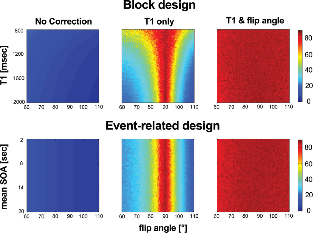
Figure 1 shows the tSNR map for the simulated time series as a function of the flip angle (60–110°). Although tSNR values in the “T1 only” correction show a significant increase only around the flip angle of 90°, tSNR values in the “T1 & flip angle” correction exhibit an increase across the entire range of flip angles, T1s, and SOA means tested. Note that the “T1 & flip angle” correction did not alter the amplitude of the BOLD signal (data not shown). This clearly indicates that the “T1 only” correction is effective only when the actual flip angle is near 90°.

FIG. 1.

Temporal SNR in simulated cardiac-gated time series for varying flip angle, T1, and mean of stimulus onset asynchrony (SOA). Top: block design for varying T1 between 800 and 2000 ms. Bottom: event-related design using jittered SOA for a range of mean SOA, from 2 s to 20 s, and T1 of 1600 ms. Although tSNR values in the “T1 only” correction show a significant increase only around the flip angle of 90°, tSNR values in the “T1 & flip angle” correction exhibit an increase across the entire range of flip angles tested.

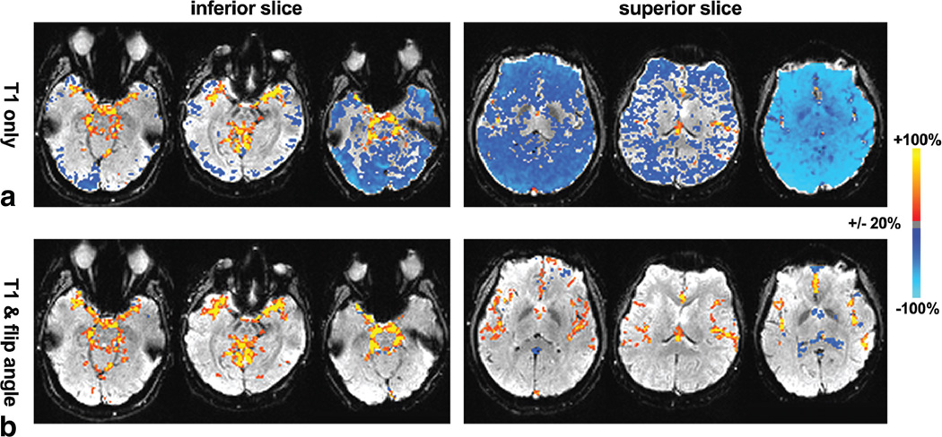
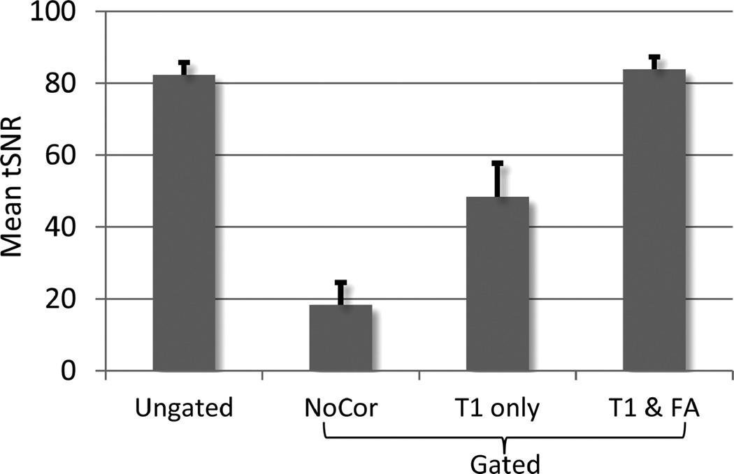
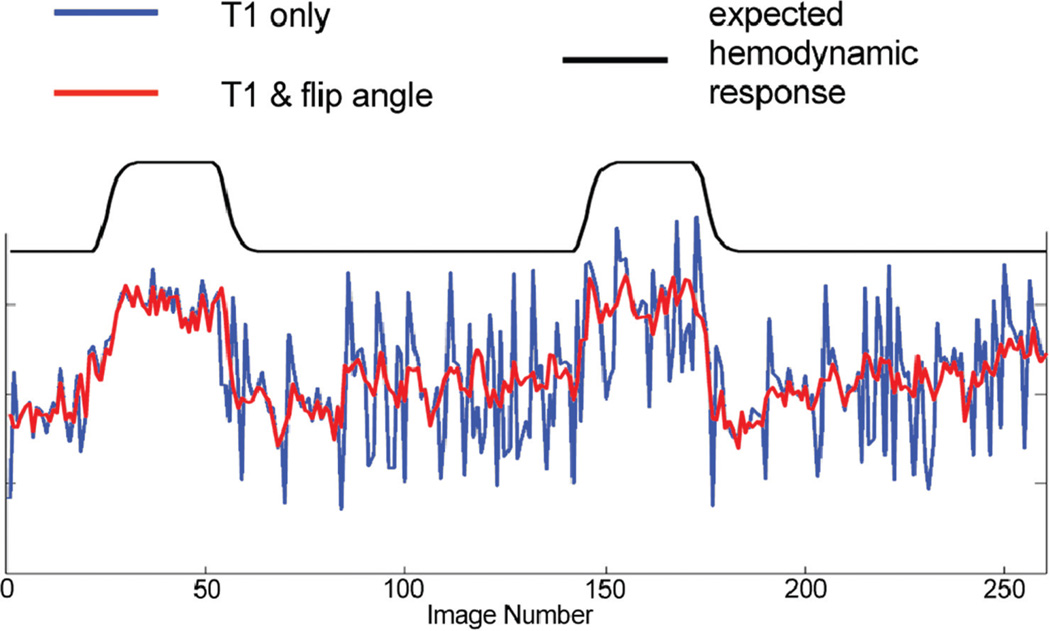
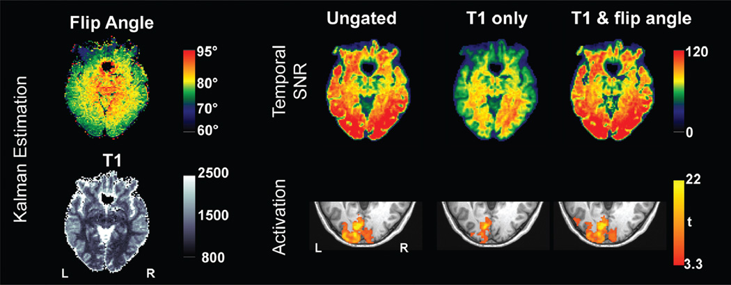
From in vivo experimental data, the percentage changes in tSNR using the two correction methods for the gated time series relative to the ungated time series are presented for three subjects in Figure 2. The increase in tSNR was observed in subcortical regions including LGN and brain stem for both correction methods compared to the ungated time series, as a result of cardiac-gated acquisition. For the “T1 only” correction, the gain comes at the expense of substantial decrease of tSNR in other brain regions. The reduction in tSNR was more prominent in superior slices (Fig. 2). This is because flip angles in superior slices (average of 73°) deviate farther from 90° than those in inferior slices (average of 83°), consistent with a previous report (8). However, the “T1 & flip angle” correction did not result in the reduction of tSNR. The tSNR averaged across grey matter for all subjects is shown in Figure 3. The result from the gated times series with the “T1 & flip angle” correction was significantly higher than that from the “T1 only” correction across all subjects (a paired t-test P < 0.004), demonstrating that the new correction improved the temporal signal stability by reducing signal fluctuations induced by variable TRs. Representative time series from experimental data are presented in Figure 4. It is evident that the fluctuations are substantially more reduced by the “T1 & flip angle” correction compared to the “T1 only” correction while the contrast of interest remains unaffected. The tSNR maps and the activation maps from a representative subject are illustrated in Figure 5, showing that tSNR in the “T1 & flip angle” correction is significantly higher than that in the “T1 only” correction. Activation results clearly demonstrate that the “T1 & flip angle” correction is more robust than the “T1 only” correction in terms of statistical significance and spatial extent. The estimated flip angle (Fig. 5) shows a wide variation, ranging from 62 to 95°, consistent with previous reports (7,8).

FIG. 2.

Changes in tSNR in the inferior slice (left) and the superior slice (right) for the gated time series with (a) “T1 only” correction and (b) “T1 & flip angle” correction compared to the conventional ungated time series for three subjects. Prominent increases were observed in regions near large vessels and subcortical regions for the gated time series. A substantial reduction was noticeable in superior slices for the “T1 only” correction. Areas where changes were less than 20% are not shown.

FIG. 3.

Grey matter tSNR, averaged from seven subjects of the ungated time series and gated time series with different correction methods. The tSNR of the “T1 only” correction was significantly lower than that of “T1 & flip angle” correction (P < 0.004). Error bars represent the standard error of the mean.

FIG. 4.

Time courses in a representative voxel in the right visual cortex derived from two different correction methods (“T1 only” vs. “T1 & flip angle”).

FIG. 5.

Results from a representative subject. Left: estimated flip angle and T1 using Kalman filter. Right: tSNR maps and activation maps for the right field stimulus at P < 0.05 (corrected).

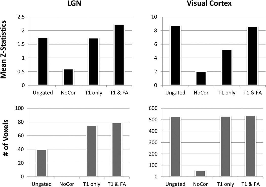
To further examine the activations in the two ROIs, we first compared the number of activated voxels at the group level of analysis. Figure 6 demonstrates that the number of activated voxels in the LGN from both correction methods for the gated time series (75 voxels for the “T1 only” and 79 voxels for the “T1 & flip angle”) is higher than that of the ungated dataset (40 voxels). A gated time series with no correction did not show any LGN activation at the group level analysis. The result indicates that correction is effective at increasing signal detection at the LGN. The effectiveness of the correction for the T1 effect was further assessed in terms of its impact on the statistics at the subject-level analysis. The t-statistic maps were converted to Z-statistics and the mean Z-statistics for different approaches were compared across subjects. The values derived from the “T1 & flip angle” correction are significantly higher than those of the “T1 only” correction across all subjects according to a paired t-test (P < 0.002), indicating that the new correction improved detection. In the visual cortex, there is no significant difference between the ungated approach and the “T1 & flip angle” approach in terms of the number of activated voxels or the mean Z-statistics. However, the “T1 only” approach led to a mean Z-score that is only 60% of those obtained with the ungated approach and the “T1 & flip angle” approach, demonstrating that the “T1 only” approach reduces the detection power in the visual cortex, due to the use of incorrect flip angle.

FIG. 6.

Comparison of the activations in the contralateral conditions in LGN and visual cortex ROIs for four different time series: (top) mean Z-statistics and (bottom) the number of activated voxels (P < 0.01, uncorrected).

DISCUSSION

This work introduces a more general technique for correcting the T1 effect in cardiac-gated fMRI that accounts for spatial variation in flip angle. The method removes T1-related signal fluctuations throughout the entire brain in the presence of B1 inhomogeneity. Cardiac-gated fMRI has been shown to improve the sensitivity of fMRI, particularly for subcortical regions that tend to move more with cardiac pulsation. Experimental results reported here demonstrate the improved detection of LGN activation with gated acquisition and T1 correction. However, the gain in the subcortical region by the “T1 only” correction is associated with a loss of sensitivity in the cortex due to the use of incorrect flip angle in the presence of B1 inhomogeneity. This loss of sensitivity is clearly seen in simulations and experimental data, particularly in the lower statistics scores (t = 5.3) in the visual cortex activation derived with the “T1 only” correction method compared to that of the ungated dataset (t = 8.7). As demonstrated by simulation and experimental results, the “T1 & flip angle” approach described here completely eliminated this loss of sensitivity and made the gated acquisition more robust.

It is challenging to study subcortical nuclei using fMRI because of their small sizes, relatively low BOLD contrast, and deep locations that are susceptible to pulsatile motion artifacts. In this study, the hemifield retinotopic relationship in the human brain was demonstrated in the LGN, the thalamic station in the projection of the visual pathway from retina to primary visual cortex. These results are consistent with earlier observations (18,19). Thus, cardiac-gated fMRI with the correction technique developed here offers opportunities for studying subcortical regions without reducing the detection power in cortical regions.

The new approach does not require additional scans to estimate the flip angle and T1. The natural variability of TR in the gated fMRI allows the estimation of the parameters directly from the acquired data using a Kalman filter. Although the transient change was ignored in Eq. 5, the Kalman filter accounts for this change as the state or measurement noise. Note that the T2* term remains in the state-space model to capture the time-varying BOLD signal. The robustness of the technique was demonstrated in simulations for both block and event-related designs. The technique of estimating the flip angle using a Kalman filter may be used in other applications where a flip angle (or B1) map is needed. It is worth noting that a Kalman filter can also be used to estimate the T2* change, s_k,3 in Eq. 12, from noisy fMRI measurements as the unobserved time-varying state estimation. In this study, we have used a Kalman filter for estimating the flip angle and T1 as unknown constants in this study. In the state estimation method, a Kalman filter eliminates not only the T1 effect, but also the measurement noise, which would result in better tSNR. However, caution should be exercised as the neural activity-related signal can be confounded with the measurement noise in a Kalman filter.

CONCLUSIONS

A technique for correcting the T1 effects in cardiac-gated fMRI data is presented here. By accounting for spatial variation in flip angle, the new method is able to remove the T1 effect robustly, in the presence of significant B1 inhomogeneity. The robustness of the technique is demonstrated with simulations and experimental data. Therefore, it is expected to be a promising tool for improving the ability to map activation in fMRI, especially in subcortical regions.

APPENDIX

Unscented Transformation

We consider the propagation of an L-dimensional random variable X through an arbitrary nonlinear function,

$$\mathbf{Y}=g(\mathbf{X})$$ [A1]

Let X have mean X̄ and covariance matrix P_X. We define a set of 2L+1 weighted samples, called sigma points {w⁽ⁱ⁾, X⁽ⁱ⁾} deterministically chosen so that they completely capture the true mean and covariance of the prior random variable X as follows:

$${\mathbf{X}}^{(0)}=\overline{\mathbf{X}}\hspace{1em}\hspace{1em}{w}^{(0)}=1/L\hspace{1em}i=0$$

$${\mathbf{X}}^{(i)}=\overline{\mathbf{X}}+{\left(\sqrt{L{\mathbf{P}}_{\mathbf{X}}}\right)}^{(i)}\hspace{1em}{w}^{(i)}=1/2L\hspace{1em}i=1,\dots ,L$$ [A2]

$${\mathbf{X}}^{(i)}=\overline{\mathbf{X}}-{\left(\sqrt{L{\mathbf{P}}_{\mathbf{X}}}\right)}^{(i)}\hspace{1em}{w}^{(i)}=1/2L\hspace{1em}i=L+1,\dots ,2L.$$

Each sigma point is now propagated through the nonlinear function

$${\mathbf{Y}}^{(i)}=f({\mathbf{X}}^{(i)})\hspace{1em}i=0,\dots ,2L$$ [A3]

and the approximated mean, covariance, and cross-covariance of Y are computed as follows:

$$\overline{\mathbf{Y}}\approx \sum _{i=0}^{2L}{w}^{(i)}{\mathbf{Y}}^{(i)}$$

$${\mathbf{P}}_{\mathbf{Y}}\approx \sum _{i=0}^{2L}{w}^{(i)}({\mathbf{Y}}^{(i)})-\overline{\mathbf{Y}}){({\mathbf{Y}}^{(i)}-\overline{\mathbf{Y}})}^T$$ [A4]

$${\mathbf{P}}_{\mathbf{X}\mathbf{Y}}\approx \sum _{i=0}^{2L}{w}^{(i)}({\mathbf{X}}^{(i)}-\overline{\mathbf{X}}){({\mathbf{Y}}^{(i)}-\overline{\mathbf{Y}})}^T$$

These estimates are accurate to the second order (third order for true gaussian priors) for any nonlinear function (12). Now, we apply the unscented transformation to the recursive Kalman filter framework.

Unscented Kalman Filter

The unscented transformation is used to approximate the optimal terms in Eq. 11 where the state random variable is redefined as the concatenation of the original state and the process and observation noise random variables. By augmenting the state random variable with the noise random variables as shown in Eq. A5, we take the uncertainty in the noise random variables into account in the same manner as we do for the state during the sigma point propagation.

$${\mathbf{S}}_{a,k}={[{\mathbf{S}}_k\hspace{1em}{\mathbf{v}}_k\hspace{1em}{\mathbf{w}}_k]}^T{\mathbf{P}}_{{\mathbf{S}}_{a,k}}=\left[\begin{array}{ccc}\hfill {\mathbf{P}}_{{\mathbf{S}}_k}\hfill & \hfill 0\hfill & \hfill 0\hfill \\ \hfill 0\hfill & \hfill {\mathbf{P}}_{\mathbf{S}{\mathbf{v}}_k}\hfill & \hfill 0\hfill \\ \hfill 0\hfill & \hfill 0\hfill & \hfill {\mathbf{P}}_{w_k}\hfill \end{array}\right]$$ [A5]

Algorithmically, the unscented Kalman filter is summarized as follows (9):

1. The set of sigma points is calculated by Eq. A2 based on the augmented state random variable as Eq. [A5].

2. The transformed set is given through the MR signal model, f(·) given by Eq. 13:

   $${\mathbf{S}}_{a,k|k-1}^{(i)}=f({\mathbf{S}}_{a,k-1}^{(i)}).$$ [A6]
3. The predicted mean and covariance are computed as

   $${\mathbf{Ŝ}}_{a,k}^{-}=\sum _{i=0}^{2L}{w}_k^{(i)}{\mathbf{S}}_{a,k|k-1}^{(i)}$$

   $${\mathbf{P}}_{{\mathbf{S}}_{a,k}}^{-}=\sum _{i=0}^{2L}{w}_k^{(i)}({\mathbf{S}}_{a,k|k-1}^{(i)}-{\mathbf{Ŝ}}_{a,k}^{-}){({\mathbf{S}}_{a,k|k-1}^{(i)}-{\mathbf{Ŝ}}_{a,k}^{-})}^T.$$ [A7]
4. Each of the prediction points is instantiated through the measurement model, Eq. 14:

   $$y_{k|k-1}^{(i)}=h\left({\mathbf{S}}_{a,k|k-1}^{(i)}\right)=s_{k|k-1,4}^{(i)}.$$ [A8]
5. The predicted measurement, the innovation, covariance matrix, and the cross covariance matrix are calculated by

   $${ŷ}_k^{-}=\sum _{i=0}^{2L}{w}_k^{(i)}{y}_{k|k-1}^{(i)}$$

   $${\mathbf{P}}_{{ỹ}_k}=\sum _{i=0}^{2L}{w}_k^{(i)}{(y_{k|k-1}^{(i)}-{ŷ}_k^{-})}^2$$ [A9]

   $${\mathbf{P}}_{{\mathbf{S}}_k{ỹ}_k}=\sum _{i=0}^{2L}{w}_k^{(i)}({\mathbf{S}}_{k|k-1}^{(i)}-{\mathbf{S}}_k^{-}){(y_{k|k-1}^{(i)}-{ŷ}_k^{-})}^T,$$

   where the innovation ỹ_k is the measurement prediction error.
6. The Kalman gain is calculated by

   $${\mathbf{K}}_k={\mathbf{P}}_{{\mathbf{S}}_k,{ỹ}_k}{\mathbf{P}}_{{ỹ}_k}^{-1}.$$ [A10]
7. Finally, the update can be performed using the Kalman filter equations:

   $${\mathbf{Ŝ}}_k={\mathbf{Ŝ}}_k^{-}+{\mathbf{K}}_k(y_k-{ŷ}_k^{-})$$ [A11]

   $${\mathbf{P}}_{{\mathbf{S}}_k}={\mathbf{P}}_{{\mathbf{S}}_k}^{-}-{\mathbf{K}}_k{\mathbf{P}}_{{ỹ}_k}{\mathbf{K}}_k^T.$$

REFERENCES

- 1.Dagli MS, Ingeholm JE, Haxby JV. Localization of cardiac-induced signal change in FMRI. Neuroimage. 1999;9:407–415. doi: 10.1006/nimg.1998.0424. [DOI] [PubMed] [Google Scholar]
- 2.Glover GH, Li TQ, Ress D. Image-based method for retrospective correction of physiological motion effects in FMRI: RETROICOR. Magn Reson Med. 2000;44:162–167. doi: 10.1002/1522-2594(200007)44:1<162::aid-mrm23>3.0.co;2-e. [DOI] [PubMed] [Google Scholar]
- 3.Hu X, Le TH, Parrish T, Erhard P. Retrospective estimation and correction of physiological fluctuation in functional MRI. Magn Reson Med. 1995;34:201–202. doi: 10.1002/mrm.1910340211. [DOI] [PubMed] [Google Scholar]
- 4.Guimaraes AR, Melcher JR, Talavage TM, Baker JR, Ledden P, Rosen BR, Kiang NYS, Fullerton BC, Weisskoff RM. Imaging subcortical auditory activity in humans. Hum Brain Mapp. 1998;6:33–41. doi: 10.1002/(SICI)1097-0193(1998)6:1<33::AID-HBM3>3.0.CO;2-M. [DOI] [PMC free article] [PubMed] [Google Scholar]
- 5.Griffiths TD, Uppenkamp S, Johnsrude I, Josephs O, Patterson RD. Encoding of the temporal regularity of sound in the human brainstem. Nat Neurosci. 2001;4:633–637. doi: 10.1038/88459. [DOI] [PubMed] [Google Scholar]
- 6.DuBois RM, Cohen MS. Spatiotopic organization in human superior colliculus observed with FMRI. Neuroimage. 2000;12:63–70. doi: 10.1006/nimg.2000.0590. [DOI] [PubMed] [Google Scholar]
- 7.Jiru F, Klose U. Fast 3D radiofrequency field mapping using echo-planar imaging. Magn Reson Med. 2006;56:1375–1379. doi: 10.1002/mrm.21083. [DOI] [PubMed] [Google Scholar]
- 8.Lutti A, Hutton C, Finsterbusch JN, Helms G, Weiskopf N. Optimization and validation of methods for mapping of the radiofrequency transmit field at 3T. Magn Reson Med. 2010;64:229–238. doi: 10.1002/mrm.22421. [DOI] [PMC free article] [PubMed] [Google Scholar]
- 9.Julier SJ, Uhlmann JK. Unscented filtering and nonlinear estimation. Proceedings of the IEEE. 2004;92:401–422. [Google Scholar]
- 10.Haacke EM, Brown RW, Thompson MR, Venkatesan R. Magnetic resonance imaging: physical principles and sequence design. New York: Wiley-Liss; 1999. [Google Scholar]
- 11.Buxton RB, Wong EC, Frank LR. Dynamics of blood flow and oxygenation changes during brain activation: the balloon model. Magn Reson Med. 2005;39:855–864. doi: 10.1002/mrm.1910390602. [DOI] [PubMed] [Google Scholar]
- 12.Van Der Merwe R. Ph.D. dissertation. Beaverton, OR: Oregon Health & Science University; 2004. Sigma-point Kalman filters for probabilistic inference in dynamic state-space models. [Google Scholar]
- 13.Havlicek M, Friston KJ, Jan J, Brazdil M, Calhoun VD. Dynamic modeling of neuronal responses in fMRI using cubature Kalman filtering. NeuroImage. 2011;56:2109–2128. doi: 10.1016/j.neuroimage.2011.03.005. [DOI] [PMC free article] [PubMed] [Google Scholar]
- 14.Kalman RE. A new approach to linear filtering and prediction problems. J Basic Eng. 1960;82:35–45. [Google Scholar]
- 15.Uhlmann JK. Transfer Thesis. Oxford, UK: Univ. Oxford; 1994. Simultaneous map building and localization for real time applications. [Google Scholar]
- 16.Friston KJ, Glaser DE, Henson RNA, Kiebel S, Phillips C, Ashburner J. Classical and Bayesian inference in neuroimaging: applications. Neuroimage. 2002;16:484–512. doi: 10.1006/nimg.2002.1091. [DOI] [PubMed] [Google Scholar]
- 17.Friston KJ, Zarahn E, Josephs O, Henson RNA, Dale AM. Stochastic designs in event-related FMRI. Neuroimage. 1999;10:607–619. doi: 10.1006/nimg.1999.0498. [DOI] [PubMed] [Google Scholar]
- 18.Schneider KA, Richter MC, Kastner S. Retinotopic organization and functional subdivisions of the human lateral geniculate nucleus: a high-resolution functional magnetic resonance imaging study. J Neurosci. 2004;24:8975–8985. doi: 10.1523/JNEUROSCI.2413-04.2004. [DOI] [PMC free article] [PubMed] [Google Scholar]
- 19.Chen W, Zhu XH, Thulborn KR, Ugurbil K. Retinotopic mapping of lateral geniculate nucleus in humans using functional magnetic resonance imaging. Proc Natl Acad Sci USA. 1999;96:2430–2494. doi: 10.1073/pnas.96.5.2430. [DOI] [PMC free article] [PubMed] [Google Scholar]