Modelling non-symmetric collagen fibre dispersion in arterial walls

Abstract

New experimental results on collagen fibre dispersion in human arterial layers have shown that the dispersion in the tangential plane is more significant than that out of plane. A rotationally symmetric dispersion model is not able to capture this distinction. For this reason, we introduce a new non-symmetric dispersion model, based on the bivariate von Mises distribution, which is used to construct a new structure tensor. The latter is incorporated in a strain-energy function that accommodates both the mechanical and structural features of the material, extending our rotationally symmetric dispersion model (Gasser et al. 2006 J. R. Soc. Interface 3, 15–35. (doi:10.1098/rsif.2005.0073)). We provide specific ranges for the dispersion parameters and show how previous models can be deduced as special cases. We also provide explicit expressions for the stress and elasticity tensors in the Lagrangian description that are needed for a finite-element implementation. Material and structural parameters were obtained by fitting predictions of the model to experimental data obtained from human abdominal aortic adventitia. In a finite-element example, we analyse the influence of the fibre dispersion on the homogeneous biaxial mechanical response of aortic strips, and in a final example the non-homogeneous stress distribution is obtained for circumferential and axial strips under fixed extension. It has recently become apparent that this more general model is needed for describing the mechanical behaviour of a variety of fibrous tissues.

1. Introduction

Physiological and pathological changes in the cardiovascular system directly influence the mechanical behaviour of arterial walls [1]. It is, therefore, of crucial importance to improve understanding of the mechanical properties of the constituents of arterial walls, including the inherent features of anisotropy and nonlinearity. These properties, among others, pose formidable challenges in the constitutive modelling and numerical analysis of such tissues and can be clearly connected to the underlying structure of the tissues. The passive mechanical behaviour of an arterial wall is governed mainly by the matrix material (which consists of water, elastin, proteoglycans, etc.) and the collagen fibre reinforcement. The anisotropy is associated with the local mean alignment of the collagen fibres, which also stiffen their response when under tension, leading to their significant nonlinear characteristics. The fibres are not perfectly aligned but are dispersed around their mean direction, and the amount and character of the dispersion depends on the topography, the particular layer of the vessel considered and the respective (patho)physiological condition, inter alia. Fibre dispersion in arterial walls has been documented and analysed in, for example, [2–5]; for an overview of the structural quantification of collagen fibres in arterial walls, see [6]. In particular, the study in [5] identified the presence of two fibre families in the intima, media and adventitia of human aortas; they are helically and almost symmetrically arranged with respect to the cylinder axis. Often a third and sometimes a fourth family is present in the intima in the respective axial and circumferential directions. Recent work [7] has revealed that, while helical fibre structures are present in human elastic arteries, in more muscular arteries (as for the murine basilar artery) and veins (such as the porcine jugular vein) a transition from the helical arrangement to two nearly orthogonal fibre families aligned in the circumferential and axial directions can be observed, and it is suggested that this is to ensure optimal efficiency of the vasculature. Observations of dispersion for other tissues, including the myocardium, corneas and articular cartilage, can be found in [8,9], [10,11] and [12], respectively.

Several mechanical models accounting for the dispersion of collagen fibres have been proposed. Fibre dispersion can be represented either directly by incorporation in a strain-energy function via a probability density function (PDF) or by a generalized structure tensor, for example. Following [13], these two approaches are referred to as ‘angular integration’ (AI) and ‘generalized structure tensor’ (GST). Cortes et al. [13] compared the results of the two formulations on the basis of the energy function introduced in [14] and the GST in [15]. As was pointed out in, for example, [16] one approach is to consider the strain energy w(λ) of a single collagen fibre as a function of the fibre stretch λ and to integrate this over the unit sphere S to obtain the total free-energy function Ψ_f of the fibres per unit reference volume, i.e.

1.1

where n is the number of fibres per unit reference volume, N is a unit vector describing the orientation of an individual fibre and ρ is the relative angular density of fibres normalized according to

1.2

The region of the unit sphere where fibres are in tension is defined by the set of N for which λ > 1, where λ = (C : N ⊗ N)^1/2 is the stretch in the direction N, C is the right Cauchy–Green tensor and a double contraction is defined by C : N ⊗ N = (CN) · N. This is the AI approach.

In the GST approach, the energy function is associated with a GST H and is given by

1.3

where H is defined by

1.4

the latter following from (1.2).

By comparing these approaches, we see that (1.1) requires integration over the unit sphere at each point, while for the strain-energy function (1.3) no such integration is needed once H has been determined by (1.4)₁ or prescribed. On the one hand, the AI approach allows identification and exclusion of individual fibres under compression, while, on the other hand, this is not quite so straightforward on the basis of (1.4)₁. For a detailed discussion of the latter issue, see [17,18].

In chronological order, we now provide a short overview of the main existing continuum mechanical models which take fibre dispersion into account. Probably the study in [19] was the first to consider fibre dispersion in the analysis of fibrous connective tissues, with the tissue structure (fibre orientation) being accounted for in the strain energy via an orientation density function. The approach [20] incorporates a two-dimensional AI distribution in a strain-energy function based on the Beta distribution, but neglects the out-of-plane dispersion of the fibres, while a planar fibre dispersion was used in [21] with a Gaussian PDF to study the biaxial behaviour of arterial walls and aortic valves. In [22], the Gaussian distribution was used to compute the so-called splay invariants to represent two- and three-dimensional fibre dispersions, which the authors applied to aortic valve tissues.

In [14], the use of an exponential strain-energy function was motivated following [23], and this model was extended to the case of fibre dispersion in [15] based on the structure tensor (1.4)₁. Therein, we used a rotationally symmetric distribution of collagen fibres. In addition, the model [15] was applied to several other tissues, including the cornea [24] and articular cartilage [25], while, in [26], the constitutive model of [14] was applied with the fibre orientations uniformly distributed over the azimuthal angle. A structure tensor based on a planar counterpart of that in [15] was defined in [27,28] and used in [29].

A PDF based on the von Mises distribution taking account of a non-rotationally symmetric fibre dispersion and based on the micro-sphere model was suggested in [30], and an ellipsoidal distribution with a power-law strain-energy function, based on the AI formulation, was employed in [31] and applied to cartilage. Based on the AI approach with the von Mises distribution Raghupathy & Barocas [32] derived a closed-form solution for a simple exponential fibre stress–strain law and applied their model to planar biaxial extension of a bioartificial tissue. The study of Federico & Gasser [33] adopted the model of Gasser et al. [15] and included the limiting case of an in-plane arrangement of fibres following the AI approach, which was also used in [34] with a planar von Mises distribution to examine the in-plane dispersion of collagen fibres. In [35], the Bingham distribution was used and was claimed to be ‘clearly superior to the π-periodic von Mises distribution in modelling the collagen organization in vascular tissue’, which we have not found to be the case in this study. The model [15] was extended in [36] to incorporate a higher order statistical measure of dispersion in order to reduce differences between the GST and AI formulations. In a recent paper [17], we have introduced a fibre dispersion model with a weighted energy function that allows the exclusion of fibres which are under compression. The model, based on the AI approach, has been developed for plane strain and for three-dimensional deformations appropriate for finite-element implementation (see also the discussion in [18] on the exclusion of compressed fibres using the GST approach). A summary of the main models discussed above is listed in table 1.

Table 1.

Overview of the main existing continuum mechanical models which take fibre dispersion into account, listed in chronological order of appearance. The column ‘formulation’ describes the approach originally presented in the cited paper (GST, generalized structure tensor; AI, angular integration); PDF, probability density function; ‘parameters’ refer to the parameters describing the fibre dispersion (not material or any other parameters). The abbreviations ‘RS’, ‘NS’ and ‘IP’ refer to rotationally symmetric, non-symmetric and in-plane, respectively. For the parameters in some of the references listed, we have used notation from this paper for consistency.

refs	formulation	PDF	parameters	2D/3D	dispersion
Sacks [20]	AI	Beta	γ, δ	2D	IP
Driessen et al. [21]	AI	Gaussian	σ	2D	IP
Freed & Doehring [37]	AI/GST	Gaussian	σ	2D/3D	RS
Gasser et al. [15]	GST	von Mises	κ	3D	RS
Alastrué et al. [30]	AI	von Mises	various	3D	NS
Ateshian et al. [31]	AI	ellipsoidal	ξi, αi, i = 1, 2, 3	3D	NS
Raghupathy & Barocas [32]	AI	von Mises	b	2D	IP
Federico & Gasser [33]	AI	von Mises	b	3D	RS
Agianniotos et al. [34]	AI	von Mises	b	2D	IP
Gasser et al. [35]	AI	Bingham	κ1, κ2	3D	NS
Pandolfi & Vasta [36]	GST/AI	von Mises		3D	RS
Holzapfel & Ogden [17]	AI	von Mises	A, B, C, D,	2D/3D	RS/NS
Melnik et al. [18]	GST	von Mises	κ	3D	RS
this work	GST	bivariate von Mises	κip, κop	3D	RS/NS/IP

The model in [15] has proved to be very successful, but recently it was shown in [5] that an axisymmetric model of collagen fibre dispersion is not appropriate, and a more general dispersion model is required to accommodate the new findings. Hence, based on the structure tensor approach initiated in [15], we introduce here a bivariate von Mises distribution that enables the dispersion data to be captured. In particular, for arteries, the out-of-plane dispersion is relatively narrow while the in-plane dispersion is more significant. This work provides a natural extension of the constitutive setting documented in [14,15] to a more general context.

This work is structured as follows. In §2, we introduce the mathematical framework for describing fibre dispersion illustrated by the use of the bivariate von Mises distribution. This is particularly appropriate for use with the new experimental data, which indicate that the current models are not sufficiently general to capture the collagen fibre structure. Then we introduce a PDF which accounts for these experimental observations, and it is shown how the new model reproduces several special cases from the literature. The continuum mechanical framework associated with the dispersion structure introduced in §2 is presented in §3. In §4, the theory of §3 is applied in three representative numerical simulations with the aim of showing the efficacy and capability of the proposed structural model. Finally, §5 summarizes the proposed fibre dispersion model and discusses future developments of our work.

2. Mathematical representation of fibre dispersion

2.1. Structure tensor for the fibre dispersion

Motivated by the experimental results documented in [38], we introduce the coordinate system shown in figure 1, where the unit vector N is an arbitrary fibre direction in the reference (undeformed) configuration, expressed in terms of the two angles Φ and Θ by

2.1

where , and e₁, e₂, e₃ are unit rectangular Cartesian basis vectors. Locally, e₁ and e₂ define the tangential plane of a cylindrical coordinate system and e₃ the corresponding outward radial direction. For a circular cylinder, e₁ is taken to be the circumferential direction and e₂ the axial direction. Although the coordinate system is similar to that introduced in [15], there is a subtle but important difference: our approach does not involve symmetry about a preferred direction since recent experimental results [38] have suggested that the fibre dispersion is not rotationally symmetric.

Figure 1.

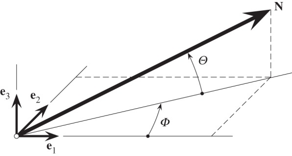
A unit vector N(Φ, Θ) representing a general fibre direction defined by the angles Φ and Θ with respect to rectangular Cartesian unit basis vectors e₁, e₂, e₃.

We describe ρ(N), which appears in (1.1), as the probability density of the fibre orientation N in the reference configuration as a function of Φ and Θ. In the following, we write either ρ(N) or ρ(Φ, Θ), and this is normalized according to (1.2), equivalently

2.2

where dS = cosΘdΦdΘ. (Note that the usual spherical polar angles are π/2 − Θ and Φ.)

Another requirement is that the PDF has to be independent of the sense of N so that ρ(N) ≡ ρ(−N), which is equivalent to ρ(Φ, Θ) = ρ(Φ + π, −Θ). Based on the experimental results presented in [38], we introduce two additional symmetries, namely the in-plane symmetry ρ(Φ, Θ) = ρ(Φ + π, Θ) and the out-of-plane symmetry ρ(Φ, Θ) = ρ(Φ, −Θ).

It is assumed that the material behaviour does not depend on the sense of N, so that the strain energy depends on N only through the tensor product N ⊗ N ([14]; see also [15,39]), via a symmetric second-order tensor, introduced in (1.4)₁, which we now write as

2.3

the components of which involve only ρ(N) and the sines and cosines of the angles Φ, Θ . The tensor H is a structure tensor involving the fibre dispersion via ρ(N). This is associated with a dispersion of fibres about a single mean direction, the mean direction of N, which, according to the data in [38], has a very small component out of plane. We therefore assume here that the mean fibre direction, say M, lies in the tangential plane defined by e₁ and e₂. An explicit expression for M will be written down below.

In terms of its components H_ij, we write H = H_ij e_i ⊗ e_j and note that, due to the symmetries of ρ(N), the off-diagonal components H₁₃ and H₂₃ vanish, and the only non-zero components of H are therefore H₁₂ and the diagonal components H₁₁, H₂₂, H₃₃. Thus, H has four non-zero components, and, because trH = 1 by (1.4)₂, only three of them are independent:

2.4

In [38], it was also observed that the dispersions in the two planes are essentially independent, which means that the PDF can be decomposed in the form

2.5

where ρ_ip(Φ) and ρ_op(Θ) describe the in-plane and out-of-plane dispersions, respectively. Since the symmetry of the PDF has to be fulfilled, we require that

Without taking explicit account of these symmetries, the normalization in equation (2.2) is now written as

2.6

Without loss of generality, we can choose the normalization of ρ_ip so that

2.7

and hence (2.6) reduces to

2.8

Let us now define

2.9

which is a measure of the out-of-plane dispersion and is consistent with the definition, in slightly different notation, given in eqn (4.1) in [15] for the case in which the dispersion is rotationally symmetric. By definition, κ_op is non-negative and from (2.8) and (2.9) it must satisfy κ_op ≤ 1/2. Thus,

2.10

If ρ_op ≡ 1, giving an isotropic distribution, then κ_op = 1/3. Note that if ρ_ip = 1 then (2.7) is automatically satisfied, but on the other hand equation (2.7) does not necessarily imply that ρ_ip = 1. However, when ρ_ip = 1 we obtain H₁₁ = H₂₂ = κ_op, H₃₃ = 1− 2κ_op and H₁₂ = 0 and this corresponds to a transversely isotropic distribution with mean fibre direction e₃. The lower limit κ_op = 0 corresponds to the case in which all the fibres are in the e₃ direction (no dispersion), while the upper limit κ_op = 1/2 corresponds to a planar distribution in the (e₁, e₂) plane. For isotropy, we have ρ_ip = ρ_op = 1 and κ_op = 1/3. In general, ρ_ip and ρ_op are separate measures of the fibre dispersions, in plane and out of plane, respectively.

We now define and by

2.11

and

2.12

and hence by (2.11)

2.13

Together, and characterize the in-plane dispersion. Note that when ρ_ip = 1 and also when the mean in-plane direction is either e₁ or e₂, as discussed below.

In general, we now have

2.14

At this point, we note that the structure tensor H has the form

2.15

and we emphasize, as noted above, that it is associated with a dispersion that has a single mean direction. We shall relate this to the model of dispersion discussed in [15] when considering special cases in §2.2.

An alternative way of writing the above representation is the form

2.16

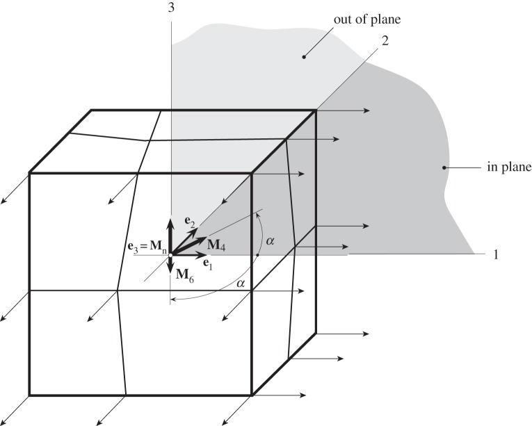
where the unit vector M = cosαe₁ + sinαe₂ is the in-plane mean fibre direction, α being the angle between M and e₁, and M_n is a unit out-of-plane vector (see figure 2), while A and B are constants.

Figure 2.

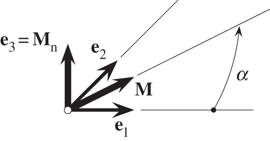
Unit vector M in the (e₁, e₂) plane, α is the angle between M and e₁, while M_n = e₃ is the unit out-of-plane vector given by e₁ × e₂.

By comparing (2.15) and (2.16), we find that the components H_ij are related to A, B and the angle α by

2.17

from which we obtain

2.18

and

2.19

By defining and , we obtain

2.20

where and depend only on the in-plane distribution. Note that is invariant with respect to the rotation of the in-plane axes.

For any given distribution ρ_ip, we can calculate and and hence the angle α and the constants and , while κ_op is obtained when ρ_op is given. Note that H contains only two independent parameters. Note also that for α = 0 or π/2 the dispersion parameter .

In §2.1.1, we consider a particular choice of the density functions ρ_ip and ρ_op.

2.1.1. Using the bivariate von Mises distribution as the dispersion distribution

The work of Schriefl et al. [38] documented angular datasets for the in-plane collagen dispersions of the intima, media and adventitia of human non-atherosclerotic thoracic and abdominal aortas and common iliac arteries. The out-of-plane angles were measured separately for each layer, showing that the out-of-plane dispersions are very similar at all anatomic locations and for each layer. Moreover, each mean fibre angle was found to be very close to tangential. Motivated by these results we now model, as illustrative examples, each of ρ_ip(Φ) and ρ_op(Θ) with π-periodic von Mises distributions [40], so the overall PDF is a bivariate von Mises distribution, featuring the symmetries that were discussed in §2.1.

For ρ_ip(Φ), we consider the basic von Mises distribution

2.21

where the so-called concentration parameter a is a constant and I₀(a) is the modified Bessel function of the first kind of order 0 defined by

2.22

which provides a normalization factor leading to (2.11) independently of a. Equation (2.22) corresponds to a distribution that is symmetric about Φ = 0. Plots of the circular distribution (2.25) for different concentration parameters a are shown in figure 3, and we note that, as a → ∞, ρ_ip becomes a delta function. For this special case of symmetry, we use the notation κ₁₁, κ₂₂ and κ₁₂. It follows from (2.25) using the definitions (2.15) and (2.16) that κ₁₂ = 0 and

2.23

where

2.24

is the modified Bessel function of the first kind of order 1.

Figure 3.

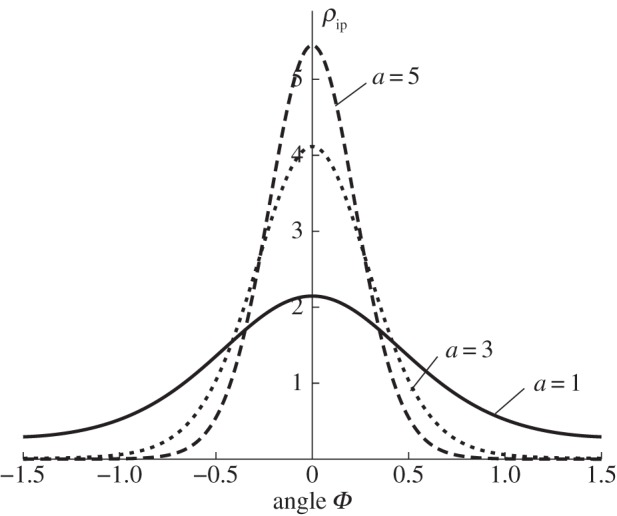
The von Mises distribution (2.21) plotted against Φ for three different values of the parameter a: (1, 3, 5), corresponding to the continuous, short dashed and long dashed curves, respectively. For a = 0 we have ρ_ip ≡ 1, while, for a → ∞, ρ_ip becomes a delta function.

If the distribution is symmetrical about Φ = α instead of Φ = 0, then Φ is replaced by Φ − α in (2.21) and the appropriate values of and are given by

2.25

and is given by (2.13). From now on, whenever κ₁₂ = 0 we use the notation κ_ip instead of κ₂₂.

Equation (2.8) is satisfied by taking ρ_op(Θ) to be a von Mises distribution of the form

2.26

where b is a constant concentration parameter and erf is the error function defined by

2.27

Note that (2.26) has a similar shape to (2.21) but is marginally different from the distribution used in [15], and gives a somewhat better fit to the narrow out-of-plane dispersion.

For the distribution (2.26), a closed-form expression for κ_op from (2.9) is obtained in the form

2.28

Figure 4 shows a plot of κ_op as a function of the concentration parameter b. Note in particular that κ_op = 1/3 when b = 0.

Figure 4.

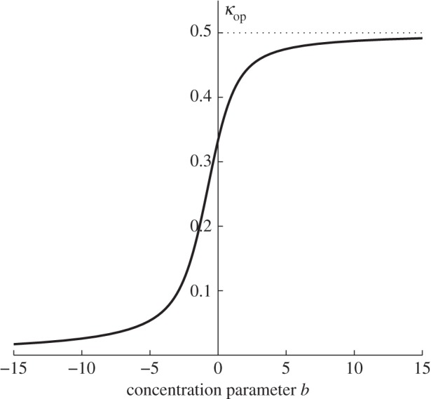
Plot of κ_op versus the concentration parameter b according to equation (2.28). Note that 0 ≤ κ_op ≤ 1/2 and κ_op = 1/3 when b = 0.

We use maximum-likelihood estimates to obtain the parameters a and b in the PDFs, ρ_ip(Φ) and ρ_op(Θ), from the angular datasets of Schriefl et al. [38]. Although it is possible to determine the parameters of a PDF by minimizing the sum of squared errors, this method has several disadvantages, as pointed out in [5], and hence we prefer to identify the parameters by using a maximum-likelihood estimate. In figure 5, we show experimental data from the adventitia of a human non-atherosclerotic abdominal aorta obtained from picrosirius polarization, in combination with a universal stage [38]. To produce the fit, we used the maximum-likelihood estimate to obtain the concentration parameters a and b. In figure 5a, we show the in-plane bi-modal distribution of ρ_ip of Φ with α = ±47.99° giving a = 2.54, which is obtained from (2.21) using Φ + α and Φ − α instead of Φ. In figure 5b, we show the out-of-plane probability density ρ_op of Θ obtained from (2.26), where b = 19.44.

Figure 5.

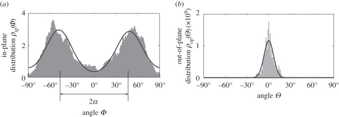
(a) Probability density ρ_ip(Φ + α), ρ_ip(Φ − α) plotted against Φ with the concentration parameter a = 2.54 and with two mean fibre directions located at α =±47.99° and (b) probability density ρ_op(Θ) against Θ with the parameter b = 19.44.

2.2. Special cases of fibre dispersions

Our model includes several existing dispersion models as special cases of (2.16), which are discussed in the following section.

2.2.1. Transversely isotropic dispersion

In [15], we considered a transversely isotropic dispersion for which H has the form

2.29

where κ is a single dispersion parameter associated with a transversely isotropic dispersion about M. Note that here we are taking M to lie in the (e₁, e₂) plane (figure 2). In [15], κ had the form

where Θ_κ is measured from M and is different from the Θ used here. The connection between Θ_κ and Θ is obtained from M · N = cosΘ_κ, with N given by (2.1) and M = cosαe₁ + sinαe₂, in the form cosΘ_κ = cosΘ cos(Φ − α).

Equation (2.29) is recovered as a special case of (2.16) by taking κ = 1 − 2κ_op, which corresponds to A = κ, B = 1 − 3κ.

2.2.2. Perfect alignment

If both concentration parameters a and b become infinite, there is no dispersion in either plane and we obtain the model proposed in [14]. With a → ∞, ρ_ip becomes an in-plane delta function, and with b → ∞ we have κ_op → 1/2. The structure tensor is then H = M ⊗ M, and all fibres are oriented in the in-plane direction of M. This corresponds to A = 0, B = 1 in (2.16).

2.2.3. Isotropic dispersion

An isotropic fibre dispersion is represented by a uniform dispersion in each plane, meaning that ρ(Φ, Θ) is independent of Φ and Θ, with ρ_ip = ρ_op = 1, so that, for the von Mises distributions, a = b = 0, while κ_op = 1/3, and the structure tensor is given by H = (1/3)I. Thus, there is no preferred direction (κ = 1/3), with A = 1/3, B = 0 in (2.16).

2.2.4. Planar dispersion

A dispersion with fibres oriented only in plane was presented in [27,39]. In this case, there is no out-of-plane contribution to H, which can be written as

2.30

where 1 is the two-dimensional identity in the considered plane with the normalization and dispersion parameter given by

2.31

Note that the normalization (2.31)₁ is equivalent to (2.7) bearing in mind the different ranges of angles used, and κ is equivalent to as defined in (2.11)₂. The in-plane PDF ρ(Θ) satisfies ρ(−Θ) = ρ(Θ). For the von Mises distribution (2.26), this corresponds to b → ∞ and κ_op → 1/2. Equation (2.30) is obtained from (2.16) by setting , B = 1−2κ. Note that this is a two-dimensional distribution but its application is not restricted to use in two dimensions.

2.2.5. Planar isotropic dispersion

If a dispersion features perfect out-of-plane alignment, b → ∞ and κ_op → 1/2, and is fully dispersed in plane so that a → 0, ρ_ip = 1, then it is planar isotropic. For this case, the structure tensor is simply H = (1/2)1, corresponding to A = 1/2, B = 0 in (2.16).

2.2.6. Summary of the special cases

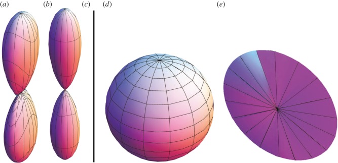
The special cases discussed above are summarized in table 2. Figure 6 is a visualization of ρ(N)N for (a) the general case for which H is given by equation (2.16), (b) the transversely isotropic dispersion given in §2.2.1 with H given by (2.29), (c) the case of perfect alignment according to §2.2.2, (d) the isotropic case according to §2.2.3 and (e) the case of planar dispersion given by equation (2.30).

Table 2.

Special cases of the present model based on the von Mises distributions (2.21) and (2.26). TI, transversely isotropic dispersion; ID, isotropic dispersion; PA, perfect alignment; PD, planar dispersion; PI, planar isotropic dispersion.

case	conc. parameter	dispersion parameter	structure tensor H	reference
TI	—	κ = 1−2κop	κI + (1−3κ)M ⊗ M	[15]
PA	a → ∞, b → ∞	κop → 1/2, κ = 0	M ⊗ M	[14]
ID	a = b = 0	κop = κ = 1/3	(1/3)I	[15,41]
PD	b → ∞	κop → 1/2,	κ1 + (1−2κ)M ⊗ M	[27,39]
PI	a → 0, b → ∞	κop → 1/2	(1/2)1	[35,39]

Figure 6.

Visualization of the fibre dispersion defined by ρ(N)N, with ρ = ρ_ip(Ψ)ρ_op(Θ) according to (2.21) and (2.26), where the distance from the centre to the surface represents the probability of finding a fibre in the direction N. The plots have been scaled differently and represent (a) a non-rotationally symmetric dispersion, (b) a rotationally symmetric dispersion, (c) perfectly aligned fibres, (d) a three-dimensional isotropic fibre dispersion and (e) a planar fibre dispersion. The planar isotropic case corresponds to a circle in (e). (Online version in colour.)

3. Continuum mechanical framework

We consider a (stress-free) reference configuration, denoted Ω₀, and a deformed (spatial) configuration, denoted Ω. The deformation map χ(X) transforms a material point X ∈ Ω₀ into a spatial point x∈Ω. With this deformation map we define the deformation gradient F(X) = ∂χ(x)/∂X and its determinant J = detF(X), where J is the local volume ratio; we require J > 0.

Following [42,43], we apply the multiplicative decomposition of F into a spherical (dilatational) part J^1/3I and a unimodular (distortional) part , with . We define the right Cauchy–Green tensor and its modified counterpart as C = F^TF and , respectively, with the related invariants I₁ = trC and .

Since we treat an artery as an elastic material, we assume the existence of a strain-energy function Ψ(C, H₄, H₆) that depends on the macroscopic deformation through C and the underlying tissue structure through the structure tensors H₄ and H₆, which describe the fibre alignment and dispersion for two fibre families. Based on (2.16), these are defined by

3.1

and M₄ and M₆ lie in the (e₁, e₂) plane, and M_n normal to that plane.

For computational purposes, we assume that it is possible to split the strain-energy function into two parts as , as shown in [5,44]. The function Ψ_vol is a purely volumetric contribution while Ψ_iso represents the energy contribution of an isochoric (volume preserving) deformation through . The second Piola–Kirchhoff stress tensor S is given by S = 2∂Ψ/∂C. Using the decoupled form of Ψ, we can identify two stress contributions so that S = S_vol + S_iso. Using well-known results from tensor analysis (e.g. [44]), and the chain rule, we obtain

3.2

where p = dΨ_vol(J)/dJ is the constitutive equation for the hydrostatic pressure and

3.3

is the so-called ‘fictitious’ isochoric second Piola–Kirchhoff stress tensor. The deviator in the Lagrangian configuration is defined by , where is a projection tensor that furnishes the correct deviatoric operator in the Lagrangian setting, and is a fourth-order identity tensor.

The related elasticity tensor in the Lagrangian description is written in the decoupled form

3.4

According to [44], we have the specification

3.5

and

3.6

In (3.5), we have used the notation , where the symbol denotes the tensor product according to the rule

3.7

and the scalar function is defined by with the constitutive equation for p given in the line after equation (3.2). In (3.6), we have also used the definitions

3.8

where is the fourth-order fictitious elasticity tensor, is the trace and is the modified projection tensor of fourth order. The related spatial stress and elasticity tensors may be derived by push-forward operations on (3.2) and (3.4)₁, respectively [44]. It should be noted here that the compressible formulation is introduced for computational purposes, and the incompressibility condition has to be enforced by a numerical scheme, one example of which is the augmented Lagrangian method (e.g. [45]).

We emphasize that for a specific material we need to specify Ψ_iso and hence to calculate its derivatives with respect to , which affects the two expressions (3.3) and (3.8)₁. In §3.1, such a specification is provided.

3.1. Anisotropic strain-energy function

Each of the structure tensors H₄ and H₆ depends on two dispersion parameters. We assume that these are the same for each fibre family. Our approach follows the work of Holzapfel et al. [14] in which the contributions Ψ_g and Ψ_f of the ground matrix (non-collagenous material) and the fibres to the strain energy are added. The artery is treated as an incompressible, elastic and fibre-reinforced material with the fibre dispersion accounted for both in plane and out of plane. Hence, superposition of energies reads

3.9

Following [14,46], we model the ground substance with a neo-Hookean material , where the parameter c is the shear modulus in the reference configuration. For the fibre contributions Ψ_fi, we adopt the exponential functions [15]

3.10

where k₁ is a parameter with the dimensions of stress and k₂ a dimensionless parameter, while

3.11

is a Green–Lagrange strain-like quantity which can be interpreted as an averaged or weighted fibre strain, depending on the fibre dispersion through the structure tensor H_i and the (isochoric) macroscopic deformation through .

Since trH_i = 1, we can write . Using the definitions (3.1) of the structure tensors H₄ and H₆, we obtain

3.12

where

3.13

The invariants and are the squares of the stretches in the directions M_i and M_n, respectively. A summary of the parameters used is provided in table 3.

Table 3.

Parameters for the proposed model.

parameter	interpretation	range	identification
c (kPa)	stiffness of (isotropic) ground matrix	(0, ∞)	mechanical tests
k1 (kPa)	parameter with dimension of stress	[0, ∞)
k2 (–)	dimensionless parameter	[0, ∞)
κip	dispersion in plane	[0, 1]	histology/imaging
κop	dispersion out of plane	[0, 1/2]
M4, M6	mean fibre directions	α ∈ [0, π/2]
Mn	normal to the mean fibre plane	—

The strain-energy function used in the proposed model reads

3.14

Following [14], we make the common assumption that the fibres do not resist any compression and are only active in tension. The invariants I_i are used as switches between fibre compression and tension so that the anisotropic part Ψ_fi only contributes to the strain energy when I₄ > 1 or I₆ > 1. If one or more of these conditions is not satisfied then the relevant part of the anisotropic function is omitted from (3.14). For example, if I₄ and I₆ are less than (or equal to) 1, then the tissue response is purely isotropic. For discussion of subtle points regarding the choice of switching criteria, see [17].

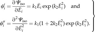
In the expressions for the stress and the elasticity tensor, we need to calculate and . By using the chain rule, these are obtained as

3.15

where H_i is given by (3.1), and we have introduced the notations

3.16

4. Representative examples

Having identified the dispersion parameters of the model in §3, we now identify the mechanical parameters by fitting the constitutive model to uniaxial data. The proposed constitutive model is then implemented in the finite-element analysis program FEAP, and the parameters obtained are used to obtain results for a simple biaxial extension of an eight-element cube and compared with the analytical (Matlab) result. Finally, numerical results are obtained for the stress distribution in the non-homogeneous extension of strips of an adventitial layer cut out along the axial and circumferential directions.

4.1. Parameter fitting to experimental data

In this example, we consider the purely incompressible formulation where the strain-energy function is characterized by Ψ = Ψ(C, H₄, H₆). The second Piola–Kirchhoff stress tensor S is then given by

4.1

where p in this case denotes the Lagrange multiplier required to enforce incompressibility. From (4.1), the Cauchy stress tensor can be computed simply by σ = FSF^T.

The strain-energy function in the present formulation reads

4.2

where

4.3

The anisotropic term in (4.2) only contributes when the fibres are extended, i.e. when I₄ > 1 or I₆ > 1. For the case that one or more of these conditions is not satisfied then the relevant part is omitted from (4.2).

We now consider a tissue specimen with two fibre families in the reference configuration with mean directions illustrated in figure 7. The unit vectors M₄ and M₆, which are symmetrically disposed in the circumferential/axial plane, each make an angle α with the circumferential direction, so that

4.4

while the normal direction to the plane is [M_n] = [0, 0, 1]^T. The deformation gradient matrix and the right Cauchy–Green matrix are

4.5

where λ₁, λ₂, λ₃ denote the principal stretches. Hence, the required invariants read

4.6

4.7

4.8

Since I_i is the same for i = 4 and 6, we obtain , where here, in analogy with (3.16)₁, , i = 4, 6. By using E_i in the strain-energy function (4.2), we obtain the derivatives of the strain-energy function as

4.9

Hence, the non-zero components of the Cauchy stress are

4.10

4.11

4.12

The constants A and B can be deduced from (2.17) and (2.18) as

4.13

Figure 7.

A specimen with two symmetric fibre families with mean fibre directions M₄ and M₆ lying in the circumferential/axial plane, each making an angle α with the circumferential direction. The normal direction to the plane is M_n.

Together with the incompressibility condition (λ₁λ₂λ₃ = 1), the implicit equations (4.10)–(4.12) with σ₂₂ = σ₃₃ = 0 can then be used to obtain p, λ₂ and λ₃ in terms of λ₁, thus giving an expression for σ₁₁ in terms of λ₁, the material parameters c, k₁ and k₂ and the structural parameters κ_ip, κ_op and α.

To determine the material parameters of our model, we use the structural data provided in figure 5 (mean fibre angle α and concentration parameters a, b) and experimental data (from uniaxial tension tests) from the adventitia of a human non-atherosclerotic abdominal aorta. A least-squares objective function is chosen as the L²-norm of the error between the model prediction of the Cauchy stress in the circumferential and the axial directions, and the corresponding experimental data. We use the function lsqnonlin in Matlab (v. R2010b; The MathWorks Inc., Natick, MA, USA), which uses the Levenberg–Marquardt algorithm to find the minimum. The dispersion parameters κ_ip from (2.23)₂ with the value of a, and κ_op from (2.28) with the value of b, can be determined from the imaging data provided in figure 5. Imaging and material data were obtained from different but comparable tissues.

To quantify the goodness of the fit, we calculate the coefficient of determination R², which is given by

4.14

where S_err and S_tot are the sums of squares of the differences between model/experiment and the mean of experiment/experiment, respectively [47]. We obtained a good fit with R² = 0.998. The parameters identified are listed in table 4. Figure 8 shows the result of fitting the proposed model to data from uniaxial tension tests.

Table 4.

Summary of material and structural parameters.

	material parameters			structural parameters
	c (kPa)	k1 (kPa)	k2 (–)	κip (–)	κop (–)	α (°)
value	10.07	5.89	21.62	0.116	0.493	±47.99°
R2		0.998		0.877	0.916	(–)

Figure 8.

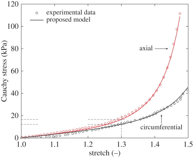
Fitting of the proposed model to the results of a uniaxial tension test. The good quality of fit is reflected in the high coefficient of determination, R² = 0.998. The model (Cauchy) stresses at a stretch of 1.3 are 16.6 (axial) and 12.2 kPa (circumferential)—see also figure 11. (Online version in colour.)

4.2. Biaxial extension: comparison of Matlab and finite-element results

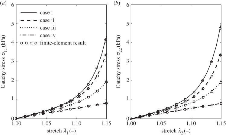
In this section, we demonstrate the efficacy of the proposed constitutive model by using eight hexahedral Q1/P0 finite elements for a cube (10 × 10 × 10), which is reinforced by two symmetric fibre families, as depicted in figure 7. The cube is subjected to homogeneous biaxial extension in the 1,2-plane, which here we call ‘in plane’, as shown in figure 9; the 2,3-plane we call ‘out of plane’. The mesh is unstructured according to figure 9. The material parameters used are those documented in table 4. We investigate four different cases of fibre dispersion: (i) structural parameters taken from table 4, which is the reference case; (ii) high alignment out of plane and isotropy in plane; (iii) less alignment out of plane and isotropy in plane; (iv) isotropy in both out of plane and in plane. For a summary see table 5.

Figure 9.

Unstructured mesh of a cube discretized by eight hexahedral finite elements. The cube is reinforced by two symmetric fibre families and subjected to homogeneous equibiaxial extension in the 1,2-plane, illustrated by arrows.

Table 5.

Four different cases of fibre dispersion for the homogeneous biaxial extension of a cube. The material parameters are taken from table 4.

case	description	dispersion parameters
i	structural parameters from table 4	κip = 0.116, κop = 0.493
ii	high alignment out of plane and isotropy in plane	κip = 0.5, κop = 0.48
iii	less alignment out of plane and isotropy in plane	κip = 0.5, κop = 0.45
iv	isotropy in out of plane and in plane	κip = 0.5, κop = 1/3

The maximum of each stretch, (λ₁, λ₂) in the 1 and 2 directions, respectively, is 1.15 and the corresponding Cauchy stresses (σ₁₁, σ₂₂) are computed from equations (4.10)–(4.12) using Matlab. In addition, these relationships are compared with results obtained from a finite-element computation using FEAP [48]. The cube is stretched simultaneously in the 1 and 2 directions under displacement-driven conditions using the Newton–Raphson method. Figure 10a,b shows plots of the Cauchy stresses σ₁₁ and σ₂₂ versus the stretches λ₁ and λ₂, respectively. Note that, for case (iv), the stresses in the 1 and 2 directions are the same since the in-plane and out-of-plane dispersions are isotropic.

Figure 10.

Homogeneous biaxial extension of a cube (cf. figure 9): (a,b) plots of Cauchy stresses σ₁₁, σ₂₂ versus stretches λ₁, λ₂ in the 1 and 2 directions. The four different cases of fibre dispersion are listed in table 5, where (i) is the reference case with parameters given in table 4. The circles represent finite-element results, while the curves are obtained from a Matlab computation.

4.3. Extension of adventitial strips

In this section, we illustrate the results of the finite-element implementation of the proposed constitutive model, simulating uniaxial extension tests related to experiments on strips performed in our laboratory in Graz, Austria. The strips were taken from an adventitial layer cut out along the axial and circumferential direction of a human non-atherosclerotic abdominal aorta. The strips, each with initial length, width and thickness of 10.0, 3.0 and 0.5 mm, respectively, were subjected to a stretch of 1.3. Both ends of each strip were constrained so as to model the mounting in the testing machine and were not allowed to deform. The resulting deformation of each strip was therefore non-homogeneous. We assume uniform material parameters over the adventitial strips with values provided in table 4. Two symmetric fibre families, as shown in figure 7, are assumed to make an angle α of ±47.99° with the circumferential direction and to show a distribution characterized by κ_ip = 0.116 and κ_op = 0.493, as also provided in table 4. We use 3200 hexahedral elements, applying the mixed Q1/P0 element throughout the simulation. Figure 11 shows the element results of the circumferential and axial specimens, subjected to a stretch of 1.3. Both circumferential and axial specimens show that the Cauchy stresses in the adventitia can be modelled within the experimentally predicted range of stresses (compare with the experimental results in figure 8). It turns out that the (axial and circumferential) stresses in the middle of the specimens are slightly higher than the model stresses provided in figure 8, which is due to the boundary conditions used in the present example.

Figure 11.

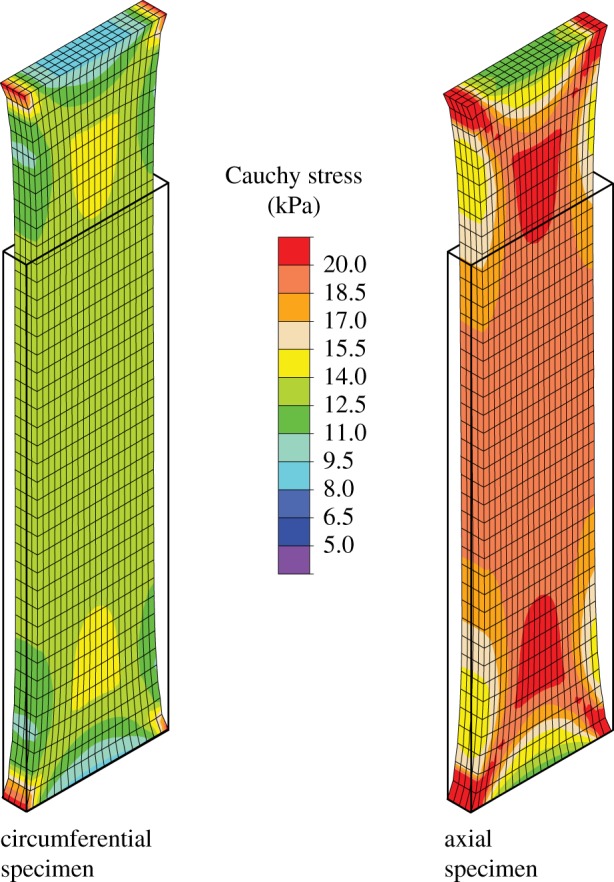
Finite-element results of circumferential and axial specimens from the adventitia, subjected to a stretch of 1.3. The Cauchy stress is plotted in the direction of the applied displacement. The undeformed (initial) configuration is indicated by solid lines.

5. Discussion

As several previous approaches have shown (e.g. [15,25,37]) incorporation of fibre dispersion into a continuum mechanical framework for soft biological tissues is a challenging and important task. Indeed the mechanical response of such tissues depends significantly on the tissue structure, in particular the arrangement of the fibre dispersion.

One of the main goals of our previous papers, e.g. [14,15], has been to incorporate the structure of biological tissues into our models in order to capture the physiological and pathological mechanical mechanisms. Recent experimental data have shown the need for a more general model that takes account of the non-symmetric arrangement of collagen fibres. This motivates the introduction, in this paper, of the bivariate von Mises distribution for describing the collagen fibre dispersion. By fitting the bivariate PDF to angular distribution data gained from imaging/histological analysis, we can determine structural parameters that can be integrated within the framework of continuum mechanics, in particular hyperelasticity. This allows us to define a strain-energy function from which the stress and the elasticity tensors can be computed, thus facilitating an efficient implementation of the model into a finite-element code.

The proposed constitutive model introduces a new structure tensor which incorporates in-plane and out-of-plane fibre dispersions in a clear and simple way, leading to an invariant-based formulation of the strain-energy function, generalizing our previous models [14,15]. The strain-energy function can incorporate different structure tensors for different fibre families. In particular, the work of Schriefl et al. [38] showed that the number of fibre families depends on the location of the artery and the type of layer, although in most cases two collagen fibre families were reported. For the most general case considered here the structure tensor has three independent components, and these reduce to two when there is in-plane symmetry (with parameters κ_ip and κ_op) or one when there is rotational symmetry about a single preferred direction (with parameter κ). Various special cases have been highlighted in §2.2, capturing the cases of rotational symmetry, in-plane dispersion, transverse isotropy and isotropy.

We have constructed a specific energy function that illustrates the efficacy of the model using three specific examples. In the first example, we have demonstrated a good fit of the model to experimental data using identified structural parameters as a fixed set. The model was then used to illustrate the effect of fibre dispersion on biaxial extension experiments, including a comparison of analytical and finite-element results. Finally, we have analysed the three-dimensional non-homogeneous stress response for a given overall extension of adventitial strips in the circumferential and axial directions obtained from a human abdominal aorta. The resulting stress responses deviate significantly from each other due to the different mechanical and structural properties in the two directions.

More data are required to determine the detailed dispersion of collagen fibres, not only for the arterial wall but also for other types of fibrous tissues. To inform the modelling process, second-harmonic generation, for example, in combination with optical clearing [49] is a powerful technique for obtaining collagen fibre dispersion data from various types of tissues.

In order to analyse the data within a continuum framework, two main approaches are used. First the AI approach, which is computationally expensive because it involves an integration over the unit sphere. It does, however, allow the exclusion of fibres undergoing compression. With the GST approach, it is possible to extract structural parameters and to include them in the continuum mechanical framework to account for the fibre dispersion. For an artery that exhibits a dispersion with a strong alignment in plane, the GST seems to be a feasible and very efficient method, although it does require a minor modification in order to exclude fibres which are under compression [18].

For further development, as mentioned above, many more data are needed to inform the modelling process. In particular, there is a pressing need to obtain in vivo data in order to construct more realistic models of tissue and organ mechanics. The model can also be extended to incorporate inelastic effects such as damage, viscoelasticity and muscle activation.

References

- 1.Díez J. 2007. Arterial stiffness and extracellular matrix. Adv. Cardiol. 44, 76–95. ( 10.1159/000096722) [DOI] [PubMed] [Google Scholar]
- 2.Canham PB, Finlay HM, Dixon JG, Boughner DR, Chen A. 1989. Measurements from light and polarised light microscopy of human coronary arteries fixed at distending pressure. Cardiovasc. Res. 23, 973–982. ( 10.1093/cvr/23.11.973) [DOI] [PubMed] [Google Scholar]
- 3.Finlay HM, McCullough L, Canham PB. 1995. Three-dimensional collagen organization of human brain arteries at different transmural pressures. J. Vasc. Res. 32, 301–312. [DOI] [PubMed] [Google Scholar]
- 4.Finlay HM, Whittaker P, Canham PB. 1998. Collagen organization in the branching region of human brain arteries. Stroke 29, 1595–1601. ( 10.1161/01.STR.29.8.1595) [DOI] [PubMed] [Google Scholar]
- 5.Schriefl AJ, Reinisch AJ, Sankaran S, Pierce DM, Holzapfel GA. 2012. Quantitative assessment of collagen fiber orientations from two-dimensional images of soft biological tissues. J. R. Soc. Interface 9, 3081–3093. ( 10.1098/rsif.2012.0339) [DOI] [PMC free article] [PubMed] [Google Scholar]
- 6.Holzapfel GA. 2008. Collagen in arterial walls: biomechanical aspects. In Collagen structure and mechanics (ed. Fratzl P.), pp. 285–324. Heidelberg, Germany: Springer. [Google Scholar]
- 7.Cyron CJ, Humphrey JD. In press. Preferred fiber orientations in healthy arteries and veins understood from netting analysis. Math. Mech. Solids. ( 10.1177/1081286514551495) [DOI] [Google Scholar]
- 8.Karlon WJ, Covell JW, McCulloch AD, Hunter JJ, Omens JH. 1998. Automated measurement of myofiber disarray in transgenic mice with ventricular expression of ras. Anat. Rec. 252, 612–625. () [DOI] [PubMed] [Google Scholar]
- 9.Covell JW. 2008. Tissue structure and ventricular wall mechanics. Circulation 118, 699–701. ( 10.1161/CIRCULATIONAHA.108.797399) [DOI] [PubMed] [Google Scholar]
- 10.Boote C, Dennis S, Meek K. 2004. Spatial mapping of collagen fibril organisation in primate cornea—an X-ray diffraction investigation. J. Struct. Biol. 146, 359–367. ( 10.1016/j.jsb.2003.12.009) [DOI] [PubMed] [Google Scholar]
- 11.Boote C, Dennis S, Huang Y, Quantock AJ, Meek KM. 2005. Lamellar orientation in human cornea in relation to mechanical properties. J. Struct. Biol. 149, 1–6. ( 10.1016/j.jsb.2004.08.009) [DOI] [PubMed] [Google Scholar]
- 12.Lilledahl MB, Pierce DM, Ricken T, Holzapfel GA, de Lange Davies C. 2011. Structural analysis of articular cartilage using multiphoton microscopy: input for biomechanical modeling. IEEE Trans. Med. Imaging 30, 1635–1648. ( 10.1109/TMI.2011.2139222) [DOI] [PubMed] [Google Scholar]
- 13.Cortes DH, Lake SP, Kadlowec JA, Soslowsky LJ, Elliot DM. 2010. Characterizing the mechanical contribution of fiber angular distribution in connective tissue: comparison of two modeling approaches. Biomech. Model. Mechanobiol. 9, 651–658. ( 10.1007/s10237-010-0194-x) [DOI] [PMC free article] [PubMed] [Google Scholar]
- 14.Holzapfel GA, Gasser TC, Ogden RW. 2000. A new constitutive framework for arterial wall mechanics and a comparative study of material models. J. Elasticity 61, 1–48. ( 10.1023/A:1010835316564) [DOI] [Google Scholar]
- 15.Gasser TC, Ogden RW, Holzapfel GA. 2006. Hyperelastic modelling of arterial layers with distributed collagen fibre orientations. J. R. Soc. Interface 3, 15–35. ( 10.1098/rsif.2005.0073) [DOI] [PMC free article] [PubMed] [Google Scholar]
- 16.Holzapfel GA, Unterberger MJ, Ogden RW. 2014. An affine continuum mechanical model for cross-linked F-actin networks with compliant linker proteins. J. Mech. Behav. Biomed. Mater. 38, 78–90. ( 10.1016/j.jmbbm.2014.05.014) [DOI] [PubMed] [Google Scholar]
- 17.Holzapfel GA, Ogden RW. 2015. On the tension–compression switch in soft fibrous solids. Eur. J. Mech. A/Solids 49, 561–569. ( 10.1016/j.euromechsol.2014.09.005) [DOI] [Google Scholar]
- 18.Melnik AV, Borja Da Rocha H, Goriely A. In press On the modeling of fiber dispersion in fiber-reinforced elastic materials. Int. J. NonLinear Mech. ( 10.1016/j.ijnonlinmec.2014.10.006) [DOI] [Google Scholar]
- 19.Lanir Y. 1983. Constitutive equations for fibrous connective tissues. J. Biomech. 16, 1–12. ( 10.1016/0021-9290(83)90041-6) [DOI] [PubMed] [Google Scholar]
- 20.Sacks MS. 2003. Incorporation of experimentally-derived fiber orientation into a structural constitutive model for planar collagenous tissues. J. Biomech. Eng. 125, 280–287. ( 10.1115/1.1544508) [DOI] [PubMed] [Google Scholar]
- 21.Driessen NJB, Bouten CVC, Baaijens FPT. 2005. A structural constitutive model for collagenous cardiovascular tissue incorporating the angular fiber distribution. J. Biomech. Eng. 127, 494–503. ( 10.1115/1.1894373) [DOI] [PubMed] [Google Scholar]
- 22.Freed AD, Einstein DR, Vesely I. 2005. Invariant formulation for dispersed transverse isotropy in aortic heart valves: an efficient means for modeling fiber splay. Biomech. Model. Mechanobiol. 4, 100–117. ( 10.1007/s10237-005-0069-8) [DOI] [PubMed] [Google Scholar]
- 23.Fung YC. 1967. Elasticity of soft tissues in simple elongation. Am. J. Physiol. 213, 1532–1544. [DOI] [PubMed] [Google Scholar]
- 24.Pandolfi A, Holzapfel GA. 2008. Three-dimensional modeling and computational analysis of the human cornea considering distributed collagen fibril orientations. J. Biomech. Eng. 130, 061006 ( 10.1115/1.2982251) [DOI] [PubMed] [Google Scholar]
- 25.Pierce DM, Trobin W, Raya JG, Trattnig S, Bischof H, Glaser C, Holzapfel GA. 2010. DT-MRI based computation of collagen fiber deformation in human articular cartilage: a feasibility study. Ann. Biomed. Eng. 38, 2447–2463. ( 10.1007/s10439-010-9990-9) [DOI] [PubMed] [Google Scholar]
- 26.Kroon M, Holzapfel GA. 2008. A new constitutive model for multi-layered collagenous tissues. J. Biomech. 41, 2766–2771. ( 10.1016/j.jbiomech.2008.05.033) [DOI] [PubMed] [Google Scholar]
- 27.Ogden RW. 2009. Anisotropy and nonlinear elasticity in arterial wall mechanics. In Biomechanical modelling at the molecular, cellular and tissue levels (eds Holzapfel GA, Ogden RW.), pp. 179–258. CISM Courses and Lectures no. 508 Wien, NY: Springer. [Google Scholar]
- 28.Holzapfel GA, Ogden RW. 2010. Modelling the layer-specific three-dimensional residual stresses in arteries, with an application to the human aorta. J. R. Soc. Interface 7, 787–799. ( 10.1098/rsif.2009.0357) [DOI] [PMC free article] [PubMed] [Google Scholar]
- 29.Wang Y, Son S, Swartz SM, Goulbourne NC. 2012. A mixed von Mises distribution for modeling soft biological tissues with two distributed fiber properties. Int. J. Solids Struct. 49, 2914–2923. ( 10.1016/j.ijsolstr.2012.04.004) [DOI] [Google Scholar]
- 30.Alastrué V, Martínez MA, Menzel A, Doblaré M. 2009. On the use of non-linear transformations for the evaluation of anisotropic rotationally symmetric directional integrals. Application to the stress analysis in fibred soft tissues. Int. J. Numer. Methods Eng. 79, 474–504. ( 10.1002/nme.2577) [DOI] [Google Scholar]
- 31.Ateshian GA, Rajan V, Chahine NO, Canal CE, Hung CT. 2009. Modeling the matrix of articular cartilage using a continuous fiber angular distribution predicts many observed phenomena. J. Biomech. Eng. 131, 61003 ( 10.1115/1.3118773) [DOI] [PMC free article] [PubMed] [Google Scholar]
- 32.Raghupathy R, Barocas VH. 2009. A closed-form structural model of planar fibrous tissue mechanics. J. Biomech. 42, 1424–1428. ( 10.1016/j.jbiomech.2009.04.005) [DOI] [PMC free article] [PubMed] [Google Scholar]
- 33.Federico S, Gasser TC. 2010. Nonlinear elasticity of biological tissues with statistical fibre orientation. J. R. Soc. Interface 7, 955–966. ( 10.1098/rsif.2009.0502) [DOI] [PMC free article] [PubMed] [Google Scholar]
- 34.Agianniotis A, Rezakhaniha R, Stergiopulos N. 2011. A structural constitutive model considering angular dispersion and waviness of collagen fibres of rabbit facial veins. Biomed. Eng. Online 10, 18 ( 10.1186/1475-925X-10-18) [DOI] [PMC free article] [PubMed] [Google Scholar]
- 35.Gasser TC, Gallinetti S, Xing X, Forsell C, Swedenborg J, Roy J. 2012. Spatial orientation of collagen fibers in the abdominal aortic aneurysm's wall and its relation to wall mechanics. Acta Biomater. 8, 3091–3103. ( 10.1016/j.actbio.2012.04.044) [DOI] [PubMed] [Google Scholar]
- 36.Pandolfi A, Vasta M. 2012. Fiber distributed hyperelastic modeling of biological tissues. Mech. Mat. 44, 151–162. ( 10.1016/j.mechmat.2011.06.004) [DOI] [Google Scholar]
- 37.Freed AD, Doehring TC. 2005. Elastic model for crimped collagen fibrils. J. Biomech. Eng. 127, 587–593. ( 10.1115/1.1934145) [DOI] [PubMed] [Google Scholar]
- 38.Schriefl AJ, Zeindlinger G, Pierce DM, Regitnig P, Holzapfel GA. 2012. Determination of the layer-specific distributed collagen fiber orientations in human thoracic and abdominal aortas and common iliac arteries. J. R. Soc. Interface 9, 1275–1286. ( 10.1098/rsif.2011.0727) [DOI] [PMC free article] [PubMed] [Google Scholar]
- 39.Holzapfel GA, Ogden RW. 2010. Constitutive modelling of arteries. Proc. R. Soc. A 466, 1551–1597. ( 10.1098/rspa.2010.0058) [DOI] [Google Scholar]
- 40.Fisher NI, Lewis TL, Embleton BJJ. 1987. Statistical analysis of spherical data. Cambridge, UK: Cambridge University Press. [Google Scholar]
- 41.Holzapfel GA, Sommer G, Gasser CT, Regitnig P. 2005. Determination of layer-specific mechanical properties of human coronary arteries with non-atherosclerotic intimal thickening, and related constitutive modeling. Am. J. Physiol. Heart Circ. Physiol. 289, H2048–H2058. ( 10.1152/ajpheart.00934.2004) [DOI] [PubMed] [Google Scholar]
- 42.Flory PJ. 1961. Thermodynamic relations for highly elastic materials. Trans. Faraday Soc. 57, 829–838. ( 10.1039/tf9615700829) [DOI] [Google Scholar]
- 43.Ogden RW. 1978. Nearly isochoric elastic deformations: application to rubberlike solids. J. Mech. Phys. Solids 26, 37–57. ( 10.1016/0022-5096(78)90012-1) [DOI] [Google Scholar]
- 44.Holzapfel GA. 2000. Nonlinear solid mechanics. A continuum approach for engineering. Chichester, UK: John Wiley & Sons. [Google Scholar]
- 45.Simo JC, Taylor RL. 1991. Quasi-incompressible finite elasticity in principal stretches. Continuum basis and numerical algorithms. Comput. Meth. Appl. Mech. Eng. 85, 273–310. ( 10.1016/0045-7825(91)90100-K) [DOI] [Google Scholar]
- 46.Holzapfel GA, Weizsäcker HW. 1998. Biomechanical behavior of the arterial wall and its numerical characterization. Comp. Biol. Med. 28, 377–392. ( 10.1016/S0010-4825(98)00022-5) [DOI] [PubMed] [Google Scholar]
- 47.Montgomery DC, Runger GC. 2010. Applied statistics and probability for engineers. New York, NY: John Wiley & Sons, Ltd. [Google Scholar]
- 48.Taylor RL. 2013. FEAP—a finite element analysis program, version 8.4, user manual. Berkeley, CA: University of California at Berkeley. [Google Scholar]
- 49.Schriefl AJ, Wolinski H, Regitnig P, Kohlwein SD, Holzapfel GA. 2013. An automated approach for three-dimensional quantification of fibrillar structures in optically cleared soft biological tissues. J. R. Soc. Interface 10, 20120760 ( 10.1098/rsif.2012.0760) [DOI] [PMC free article] [PubMed] [Google Scholar]