Theory and applications of a deterministic approximation to the coalescent model

Abstract

Under the coalescent model, the random number n_t of lineages ancestral to a sample is nearly deterministic as a function of time when n_t is moderate to large in value, and it is well approximated by its expectation E[n_t]. In turn, this expectation is well approximated by simple deterministic functions that are easy to compute. Such deterministic functions have been applied to estimate allele age, effective population size, and genetic diversity, and they have been used to study properties of models of infectious disease dynamics. Although a number of simple approximations of E[n_t] have been derived and applied to problems of population-genetic inference, the theoretical accuracy of the formulas and the inferences obtained using these approximations is not known, and the range of problems to which they can be applied is not well understood. Here, we demonstrate general procedures by which the approximation n_t ≈ E[n_t] can be used to reduce the computational complexity of coalescent formulas, and we show that the resulting approximations converge to their true values under simple assumptions. Such approximations provide alternatives to exact formulas that are computationally intractable or numerically unstable when the number of sampled lineages is moderate or large. We also extend an existing class of approximations of E[n_t] to the case of multiple populations of time-varying size with migration among them. Our results facilitate the use of the deterministic approximation n_t ≈ E[n_t] for deriving functionally simple, computationally efficient, and numerically stable approximations of coalescent formulas under complicated demographic scenarios.

1. Introduction

Many coalescent distributions and expectations can be obtained by conditioning on the random number n_t of lineages at time t in the past that are ancestral to a sample of n₀ lineages at time t = 0 in the present (Figure 1). Quantities that can be obtained by conditioning on n_t include Wakeley and Hey's (1997) formula for the joint allele frequency spectrum between two populations, Takahata's (1989) formula for the probability of concordance between a gene tree and a species tree, Griffiths and Tavaré's (1998) formula for the distribution of the age of a neutral allele, Rosenberg's (2003) formulas for the probabilities of monophyly, paraphyly, and polyphyly in two populations, and many others (Takahata and Nei 1985, Hudson and Coyne 2002, Rosenberg 2002, Rosenberg and Feldman 2002, Degnan and Salter 2005, Efromovich and Kubatko 2008, Degnan 2010, Bryant et al. 2012, Helmkamp et al. 2012, Jewett and Rosenberg 2012, Wu 2012).

Figure 1.

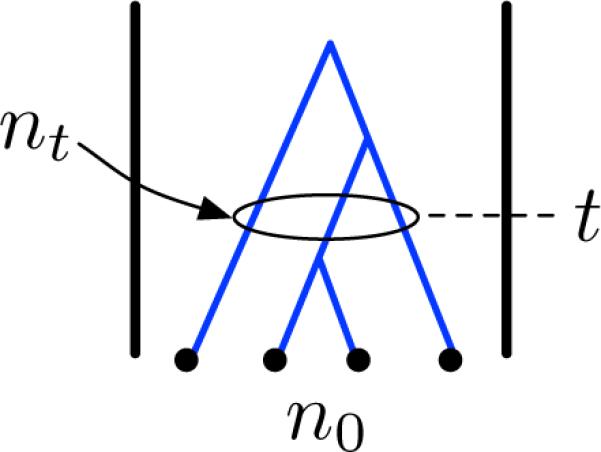
The number n_t of coalescent lineages at time t in the past that are ancestral to a set of n₀ lineages sampled at time t = 0 in the present. In this example, n₀ = 4 and n_t = 3 at the given time t.

When many lineages are sampled (and n₀ is large), summing over all possible values of n_t can be computationally expensive. As a result, evaluating formulas that condition on n_t can be computationally difficult or intractable for modern genomic datasets with hundreds or thousands of sampled alleles. In addition, formulas for the probability distribution $\mathbb{P}\left(n_t\right)$ of the number of ancestors at time t (Griffiths 1980, Donnelly 1984, Tavaré 1984) involve sums of terms of alternating sign that produce round-off error when t is small and n₀ is large (e.g. $t\lesssim {10}^{-2}$ coalescent time units and $n_0\gtrsim 50$), further complicating the evaluation of formulas that condition on n_t (Griffiths 1984).

When computing formulas that depend on the distribution $\mathbb{P}\left(n_t\right)$, round-off error can be eliminated by using asymptotic approximations of $\mathbb{P}\left(n_t\right)$ that were derived by Griffiths (1984), or by using an alternative expression for $\mathbb{P}\left(n_t\right)$ (Griffiths 2006). However, as we will discuss, approximations to coalescent formulas obtained by this approach may have similar computational complexities to the exact formulas, and can therefore be computationally slow or intractable on large data sets. Therefore, it is of interest to devise general procedures for deriving approximate coalescent formulas without requiring conditional sums over all possible values of n_t.

One alternative to summing over n_t is to use an approximation in which n_t is assumed to be equal to its expected value E[n_t] with probability one. This approximation was used by Slatkin (2000) to address the problem of round-off error in the distribution $\mathbb{P}\left(n_t\right)$ and by Volz et al. (2009) to obtain approximate distributions of coalescent waiting times. The approximation can greatly reduce the complexity of computing coalescent formulas by reducing the number of different values of n_t over which conditional summations must be computed (Jewett and Rosenberg 2012).

The surprising fact is that approximations of this kind are often very accurate because n_t changes almost deterministically over time and is well approximated by its expected value (Watterson 1975, Slatkin 2000, Maruvka et al. 2011). In fact, Maruvka et al. (2011) demonstrated that the deterministic nature of n_t is apparent even when the number n_t of ancestral lineages is not large. From Figure 2, it can be seen that the variance in n_t increases as the number of ancestral lineages decreases, with n_t deviating most from E[n_t] when $n_t\lesssim 30$ in the example shown. However, n_t is well approximated by its mean when t is small. E[n_t] is also a good approximation of n_t as t → ∞ and both n_t and E[n_t] approach unity. Thus, the approximation n_t ≈ E[n_t] can be used to obtain approximations of coalescent distributions that are computationally fast, numerically stable, and accurate for a broad range of sample sizes n₀.

Figure 2.

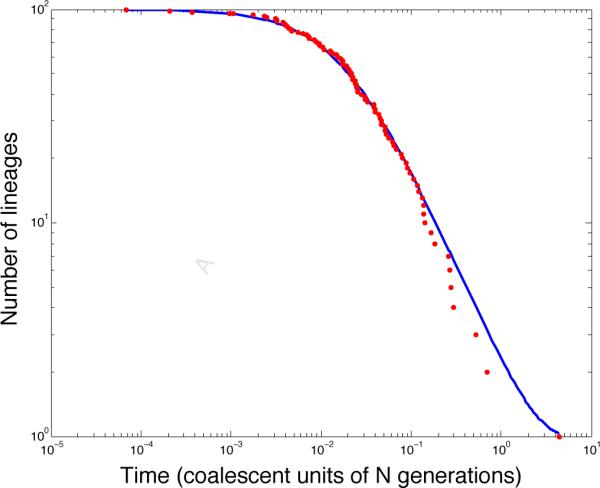
The deterministic nature of the number of ancestral lineages n_t at time t in the past. Red dots indicate the number of lineages remaining at each coalescent event in a single genealogy of n₀ = 100 lineages sampled from a population of constant size under the coalescent model. The expectation E[n_t] computed using Equation (13) is shown in blue. It can be seen that n_t is well-approximated by its expected value.

In addition to deriving fast and numerically stable approximations to coalescent formulas, the approximation n_t ≈ E[n_t] can be combined with simple approximate formulas for E[n_t] (Slatkin and Rannala 1997, Slatkin 2000, Rauch and Bar-Yam 2005, Volz et al. 2009, Frost and Volz 2010, Maruvka et al. 2011) to derive functionally simple approximate expressions for coalescent quantities (Slatkin 2000, Volz et al. 2009, Jewett and Rosenberg 2012).

Despite the utility of the approximation n_t ≈ E[n_t], it is not widely known and general procedures for applying it to obtain approximate coalescent formulas have not been developed. Moreover, the theoretical accuracy of the approximate formulas is not well understood. Here, we discuss general approaches by which the approximation n_t ≈ E[n_t] can be applied to obtain functionally simple, computationally efficient, and numerically stable approximations of coalescent distributions. We show that the resulting approximate formulas converge to their true values under simple assumptions, and we derive approximate expressions for the error. We also discuss methods for approximating E[n_t] under demographic models that include multiple populations of time-varying size with migration among them. Our results facilitate the use of the approximation n_t ≈ E[n_t] for obtaining computationally fast and numerically stable formulas that can be applied to facilitate coalescent computations on large genomic data sets with complicated demographic histories.

2. Approximating formulas that condition on n_t

2.1. Difficulties of computing coalescent formulas

We first consider applications of the approximation n_t ≈ E[n_t] to the problem of reducing the computational complexity and numerical instability of coalescent formulas that are derived by conditioning on n_t at a particular time t in the past. In particular, we consider functions of the form

$$f\left(x\right)=\sum _{{\mathbf{n}}_t}f(x\mid {\mathbf{n}}_t)\mathbb{P}\left({\mathbf{n}}_t\right),$$ (1)

where n_t = (n_1,t, ..., n_k,t) is a vector describing the number of ancestors of each of k different sets of sampled alleles with initial sample sizes ${\left\{n_{i,0}\right\}}_{i=1}^k$. The sets of lineages of ${\left\{n_{i,0}\right\}}_{i=1}^k$ can be drawn from different populations, but they can also come from the same population. Here, f(x) is a quantity of interest that we wish to compute, such as an expectation parameterized by a variable x or a probability distribution function for a random variable X. The sum is carried out over k variables, one for each entry in n_t, and the ith sum proceeds from 1 to n_i,0.

Two primary difficulties arise when evaluating functions of the form in Equation (1). First, summing over all values of n_t can be computationally expensive, making conditional formulas computationally intractable when many lineages are sampled. Second, for any given number of sampled alleles, i, the distribution $\mathbb{P}\left(n_{i,t}\right)$ of the number of ancestors is given by a complicated expression

$$\mathbb{P}\left(n_{i,t}\right)=\sum _{j=n_{i,t}}^{n_{i,0}}\frac{{(-1)}^{j-n_{i,t}}(2j-1){\left(n_{i,t}\right)}_{(j-1)}{\left(n_{i,0}\right)}_{\left[j\right]}}{n_{i,t}!(i-n_{i,t})!{\left(n_{i,0}\right)}_{\left(j\right)}}{e}^{-\left(\begin{array}{c}\hfill j\hfill \\ \hfill 2\hfill \end{array}\right)t},$$ (2)

where $n_{\left[j\right]}=n!∕(n-j)!$ and $n_{\left(j\right)}=(n+j-1)!∕(n-1)!$ and where time, t, is in coalescent units of N generations (Tavaré 1984). Due to terms of alternating sign in Equation (2), this distribution is subject to round-off error when $n_0\gtrsim 50$ and $t\lesssim {10}^{-2}$, making calculations inaccurate. Therefore, because of difficulties with computational complexity and numerical instability, it is of interest to find other means of evaluating formulas of the form given in Equation (1).

2.1.1. The Griffiths approximation

One approach for eliminating round-off error in coalescent formulas of the form given in Equation (1) is to use a set of asymptotic approximations derived by Griffiths (1984). Griffiths showed that as n₀ → ∞ and t → 0, n_t has an asymptotically normal distribution. He derived expressions for the asymptotic mean μ_t and variance ${\sigma }_t^2$ of this distribution. Griffiths’ asymptotic formulas can be used to obtain numerically stable approximations to formulas of the form given in Equation (1) by replacing the distribution $\mathbb{P}\left(n_{i,t}\right)$ (i = 1, .., k) with the corresponding asymptotic normal distribution (Chen and Chen 2013). Using Griffiths’ asymptotic formulas, the approximation of Equation (1) is

$$f\left(x\right)=\sum _{{\mathbf{n}}_t}f(x\mid {\mathbf{n}}_t)\prod _{i=1}^k\frac{1}{\sqrt{2\pi }{\sigma }_{i,t}}{e}^{-{(n_{i,t}-{\mu }_{i,t})}^2∕\left(2{\sigma }_{i,t}^2\right)},$$ (3)

where μ_i,t and σ_i,t are the mean and variance of Griffiths’ normal approximation to the distribution $\mathbb{P}\left(n_{i,t}\right)$, and where the summation is taken over n_i,t = 1, ..., n_i,0 for i = 1, ..., k. Throughout this manuscript, we refer to an approximation of the form in Equation (3) to an exact coalescent formula of the form given in Equation (1) as the Griffiths approximation of the formula.

The asymptotic approximations derived by Griffiths are useful for eliminating round-off error when evaluating the distribution of n_t. However, although the Griffiths normal approximations are very fast to compute, the complexity of Equation (3) is similar to that of Equation (1) because the same number of terms of approximately the same complexity must be computed in both formulas. Thus, it is of interest to identify alternatives to Griffiths’ asymptotic formulas that can be used to evaluate coalescent expressions in a computationally efficient way when the sample size is large. The key challenge is to eliminate the multiple summation over ${\prod }_{i=1}^k{n}_{i,0}$ terms.

2.1.2. The deterministic approximation

We consider an alternative to Griffiths’ asymptotic formulas that is useful for reducing the computational complexity of equations of the form given in Equation (1) when the number n₀ of sampled lineages is large. The alternative is to assume that the number n_t of lineages ancestral to a given sample of n₀ alleles is equal to its expected value E[n_t] with probability 1. The result of this approximation is that the summation in Equation (1) collapses to a single term

$$f\left(x\right)=\sum _{{\mathbf{n}}_t}f(x\mid {\mathbf{n}}_t)\mathbb{P}\left({\mathbf{n}}_t\right)\approx f(x\mid E\left[{\mathbf{n}}_t\right]),$$ (4)

which is fast to evaluate. Throughout this manuscript we refer to an approximation of the form in Equation (4) to an exact coalescent formula of the form given in Equation (1) as the deterministic approximation of the formula.

To our knowledge, the deterministic approximation was first used by Slatkin (2000) to treat problems with round-off error in the distribution $\mathbb{P}\left(n_{i,t}\right)$. We demonstrate here that this approximation can often be used as an alternative to Griffiths’ approximation, to reduce the computational complexity of coalescent formulas that contain terms of the form in Equation (1).

2.2. Approximating distributions that condition on the path of n_t

A more general version of the approximation in Equation (4) applies to formulas that can be obtained by conditioning on the path of the stochastic process n_t over a range of time values [r, s], rather than on the instantaneous value of the process n_t at the single time point t. In particular, consider the stochastic process n_t (0 ≤ t ≤ ∞), where the value at t = ∞ refers to the t → ∞ limit, and let n_[r,s] denote a sample path of the process on the time interval [r, s]. We consider approximations to coalescent quantities f(x) that can be expressed using formulas of the form

$$f\left(x\right)={\int }_{{\mathcal{A}}_{[r,s]})}f(x\mid {\mathbf{n}}_{[r,s]})p\left({\mathbf{n}}_{[r,s]}\right)d{\mathcal{A}}_{[r,s]},$$ (5)

where f(x|n_[r,s]) is the conditional expression for f(x) given a particular sample path n_[r,s] on the interval [r, s], ${\mathcal{A}}_{[r,s]}$ is the sample space of all paths of the stochastic process n_t on the time interval [r, s], and p(n_[r,s]) is the probability density function of these paths.

Such conditional formulas represent a wide variety of coalescent quantities. For example, consider a single set of sampled alleles (k = 1 and n_t = n_t) on the time interval [r, s] = [0, ∞). If we define the conditional function

$$f(x\mid n_{[0,\infty )})=\{\begin{array}{cc}1\hfill & \text{if}{n}_x=1\hfill \\ 0\hfill & \text{otherwise},\hfill \end{array}\phantom{\}}$$ (6)

then Equation (6) is an indicator random variable that takes on the value 1 if the n₀ sampled alleles find their most recent common ancestor before time x. In this case, Equation (5) is the cumulative distribution function of the time to the most recent common ancestor (TMRCA).

Alternatively, we could consider the time interval [r, s] and define the conditional function f(x|n_[r,s]) to be

$$f(x\mid n_{[r,s]})={\int }_{z=r}^s{n}_{z}dz.$$

This quantity is the total sum of branch lengths of the sample path on the time interval [r, s]. In this case, f(x) in Equation (5) is the expected branch length of the genealogy on the time interval [r, s].

2.2.1. Approximating Equation (5)

By analogy with Equation (4), quantities of the form given in Equation (5) can be approximated as

$$f\left(x\right)={\int }_{{\mathcal{A}}_{[r,s]}}f(x\mid {\mathbf{n}}_{[r,s]})p\left({\mathbf{n}}_{[r,s]}\right)d{\mathcal{A}}_{[r,s]}\approx f(x\mid E\left[{\mathbf{n}}_{[r,s]}\right]),$$ (7)

where E[n_[r,s]] is the expected sample path of the stochastic process n_t over the time interval [r, s]. Such approximations not only reduce the complexity of computing coalescent quantities by eliminating the integral over all possible paths, they also facilitate the derivation of approximate coalescent formulas that would otherwise be difficult to derive analytically.

2.2.2. An application of Equation (7)

For a single sample of n₀ alleles, specifying the term f(x|n_[r,s]) in Equation (7) by $f(x\mid n_{[r,s]})={\int }_{z=r}^s{n}_z{d}_z$ is particularly useful for computing quantities that depend on the expected number of segregating sites in all or in part of a genealogy. In particular, under the infinitely-many-sites model, the expected number of mutations S on a genealogy at a locus of length b bases is proportional to the expected total branch length L of the genealogy:

$$E\left[S\right]=E\left[E[S\mid L]\right]=E[\theta bL∕4]=\frac{\theta b}{4}E\left[L\right],$$ (8)

where θ = 4Nμ is the population-scaled mutation rate per-site per-generation, N is a specified effective population size, μ is the per-site per-generation mutation rate, and L is given in units of N generations. If L_[r,s] is the total length of a genealogy over the time interval [r, s], then the number of segregating sites S_[r,s] in the interval is

$$E\left[S_{[r,s]}\right]=\frac{\theta b}{4}E\left[L_{[r,s]}\right].$$ (9)

The expectation on the right-hand side of Equation (9) can be computed using the following theorem:

Theorem 2.1. Let L_[r,s] be the total sum of branch lengths of the genealogy of n₀ sampled alleles in the time interval [r, s] with 0 ≤ r ≤ s ≤ ∞. Then the expectation E[L_[r,s]] is given by

$$E\left[L_{[r,s]}\right]={\int }_{z=r}^{s}E\left[n_z\right]dz.$$ (10)

The proof of Theorem 2.1 is given in Appendix A. As we demonstrate in Section 5, Equation 10 can be used to compute quantities such as the number of mutations that are private to a given population or sample and terms in the joint allele frequency spectrum among a pair of populations. A result similar to Theorem 2.1 that considers the full genealogy up until the time to the most recent common ancestor was proved by Chen and Chen (2013).

3. The theoretical accuracy of the approximate formula

In this section we consider the accuracy of the approximate coalescent formula obtained using Equation (4). In comparison with Griffiths’ approximation (Equation 3), which was shown to converge to the correct value in the double limit as n₀ increases to infinity and t decreases to zero (Griffiths 1984), we show that the deterministic approximation (Equation 4) of a coalescent formula converges to the true value as t → 0 and as t → ∞ with the value of n₀ fixed. As we will see, these less stringent criteria for convergence often allow the deterministic approximation to be more accurate than the Griffiths approximation when the sample size n₀ is small. The accuracy of the deterministic approximation is formalized in the following theorem.

Theorem 3.1. Suppose that a function f(x) can be expressed as $f\left(x\right)={\sum }_{{\mathbf{n}}_t}f(x\mid {\mathbf{n}}_t)\mathbb{P}\left({\mathbf{n}}_t\right)$, where f(x|n_t) is defined for all x in some domain $D\subseteq \mathbb{R}$ and for $n_{i,t}\in {\mathcal{N}}_i=[1,n_{i,0}](i=1,\dots ,k)$. Suppose that the second-order partial derivatives $\frac{{\partial }^2}{\partial n_{i,t}\partial n_{j,t}}f(x\mid {\mathbf{n}}_t)$ exist and are continuous and bounded in n_i,t (i = 1, ..., k) for all x ∈ D and for ${\mathbf{n}}_t\in \mathcal{N}={\mathcal{N}}_1\times \cdots \times {\mathcal{N}}_k$ Then for a fixed value of n₀, f(x[notdef]E[n_t]) converges uniformly to f(x) on D as t → 0 and as t → ∞.

The proof of Theorem 3.1 follows from a lemma proved in Appendix B and is given in Appendix C. We also obtain an approximate expression for the error in the deterministic approximation as t → 0 and as t → ∞. In particular, we show that the error |f(x) − f(x|E[n_t])| is given approximately by

$$\mid f\left(x\right)-f(x\mid E\left[{\mathbf{n}}_t\right])\mid \approx \frac{1}{2}\mid \sum _{i=1}^k\sum _{j=1}^k\mathrm{Cov}(n_{i,t},n_{j,t})\frac{{\partial }^2}{\partial n_{i,t}\partial n_{j,t}}f(x\mid E\left[{\mathbf{n}}_t\right])\mid$$ (11)

as t → 0 and as t → ∞ (Appendix D). In the commonly-occurring scenario in which the numbers of ancestors n_i,t (i = 1, .., k) are independent of one another, Equation (11) reduces to

$$\mid f\left(x\right)-f(x\mid E\left[{\mathbf{n}}_t\right])\mid =\frac{1}{2}\mid \sum _{i=1}^k\mathrm{Var}\left(n_{i,t}\right)\frac{{\partial }^2}{\partial n_{i,t}^2}f(x\mid E\left[{\mathbf{n}}_t\right])\mid ,$$ (12)

Equation (12) can be evaluated for any given quantity f(x) either by evaluating Tavaré's expression for Var(n_t) (Equation B.10), or by using one of the asymptotic expressions for Var(n_t) given in Theorem 2 of Griffiths (1984).

4. Approximating E[n_t]

In order to apply the approximation n_t ≈ E[n_t], it is necessary to compute E[n_t]. Chen and Chen (2013) noted that the expected value E[n_t] can be computed for a population of variable size N(t) at time t in the past using the formula derived by Tavaré (1984)

$$E[n_t\mid n_0]=\sum _{i=1}^{n_0}(2i-1)\frac{{\left(n_0\right)}_{\left[i\right]}}{{\left(n_0\right)}_{\left(i\right)}}{e}^{-\left(\begin{array}{c}\hfill i\hfill \\ \hfill 2\hfill \end{array}\right)\tau \left(t\right)},$$ (13)

where $n_{\left[i\right]}=n!∕(n-i)!$ and $n_{\left(i\right)}=(n-1+i)!∕(n-1)!$, where time t is in units of generations, and where $\tau \left(t\right)={\int }_{z=0}^{t}1∕N\left(z\right)dz$ is a rescaling of time (see Section 4.1). In a population of constant size N(t) = N, τ(t) simplifies to τ(t) = t/N. Although Equation (13) has a functionally simple form (a polynomial in e^−t), it can be slow to compute when the sample size n₀ is large, and it does not hold for complicated demographic models with migration. Because there is currently no closed-form expression for E[n_t] in the case of migration, it is of interest to obtain accurate approximations of E[n_t] in this more complicated scenario. Note that the problem of approximating E[n_t] is distinct from the problem of approximating n_t by E[n_t].

Several studies derived simple deterministic approximations of E[n_t] in a single panmictic population (Griffiths 1984, Slatkin and Rannala 1997, Rauch and Bar-Yam 2005, Volz et al. 2009, Frost and Volz 2010, Maruvka et al. 2011). With the exception of the approximations derived by Griffiths (1984), these studies all used a differential equation approach to obtain approximations of E[n_t], all employing slight variations on the same differential equation. Here, we show that this differential equation can be extended to obtain an approximation of E[n_t] under models with migration among populations.

As background for our derivation, we begin with a brief overview of approximations of E[n_t] in a single population. We also take the opportunity to compare these approximations of E[n_t] to one another in terms of their relative accuracy, and we theoretically validate these approximations by showing that they are in fact asymptotically equal to E[n_t] in certain limits.

4.1. Approximating E[n_t] in a single population

Slatkin and Rannala (1997) derived a differential equation for E[n_t] in a single population:

$$\frac{dE\left[n_t\right]}{dt}=-\left(\begin{array}{c}\hfill E\left[n_t\right]\hfill \\ \hfill 2\hfill \end{array}\right)\frac{1}{N\left(t\right)}-\frac{\mathrm{Var}\left(n_t\right)}{2N\left(t\right)},$$ (14)

where N(t) is the size of the population at time t in the past. The approximate formulas for E[n_t] derived by Slatkin and Rannala (1997), Volz et al. (2009), Frost and Volz (2010), and Maruvka et al. (2011) can each be derived by making various simplifying approximations of Equation (14). In each approximation, Var(n_t) is assumed to be much smaller than $\left(\begin{array}{c}\hfill E\left[n_t\right]\hfill \\ \hfill 2\hfill \end{array}\right)$ so that the term Var(n_t)/(2N(t)) can be neglected. Slatkin and Rannala (1997) and Volz et al. (2009) further assumed that E[n_t] >> 1 in order to obtain the approximation

$$\frac{dE\left[n_t\right]}{dt}\approx -\frac{E{\left[n_t\right]}^2}{2N\left(t\right)}.$$ (15)

Frost and Volz (2010) and Maruvka et al. (2011) retained the term $-E\left[n_t\right]∕\left(2N\left(t\right)\right)$, obtaining the approximation

$$\frac{dE\left[n_t\right]}{dt}\approx -\left(\begin{array}{c}\hfill E\left[n_t\right]\hfill \\ \hfill 2\hfill \end{array}\right)\frac{1}{N\left(t\right)}.$$ (16)

Equations (15) and (16) can both be simplified further by using a trick implemented by Slatkin and Rannala (1997). In particular, Griffiths and Tavaré (1994) showed that the distribution of the number of ancestral lineages at time t generations in a population of time-varying size N(t) is the same as the distribution of the number of ancestral lineages in a constant population of size N = 1 at time $\tau \left(t\right)={\int }_{z=0}^{t}1∕N\left(z\right)dz$. Thus, Slatkin and Rannala (1997) noted, it is sufficient to solve Equations (15) and (16) for the case of N = 1 and then evaluate the solution at time τ(t). This approach yields the solution

$$E\left[n_t\right]\approx \frac{n_0}{1+n_0\tau \left(t\right)∕2}$$ (17)

for Equation (15) and the solution

$$E\left[n_t\right]\approx \frac{n_0}{n_0+(1-n_0)e^{-\tau \left(t\right)∕2}}$$ (18)

for Equation (16). These approximations of E[n_t] are summarized in Table 1.

Table 1.

Approximations of E[n_t] with $\tau \left(t\right)={\int }_{z=0}^{t}1∕N\left(z\right)dz$.

Authors	Assumptions	Equation	Solution
Slatkin and Rannala (1997), Volz et al. (2009)	$\mathrm{Var}\left(n_t\right)\ll E\left[n_t\right],E\left[n_t\right]\gg 1$	$\frac{d}{dt}E\left[n_t\right]\approx -\frac{E{\left[n_t\right]}^2}{2}$	$E\left[n_t\right]\approx \frac{n_0}{1+n_0\tau \left(t\right)∕2}$
Frost and Volz (2010), Maruvka et al. (2011)	$\mathrm{Var}\left(n_t\right)\ll E\left[n_t\right]$	$\frac{d}{dt}E\left[n_t\right]\approx -\left(\begin{array}{c}\hfill E\left[n_t\right]\hfill \\ \hfill 2\hfill \end{array}\right)$	$E\left[n_t\right]\approx \frac{n_0}{n_0+(1-n_0)e^{-\tau \left(t\right)∕2}}$
This paper	$\mathrm{Var}\left(n_t\right)\ll E\left[n_t\right]$	$\frac{d}{dt}E\left[n_{\ell t}\right]\approx -\left(\begin{array}{c}\hfill E\left[n_{\ell t}\right]\hfill \\ \hfill 2\hfill \end{array}\right)+{\sum }_{\begin{array}{c}\hfill i=1\hfill \\ \hfill i\ne \ell \hfill \end{array}}^k(E\left[n_{it}\right]m_{i\ell }-E\left[n_{\ell t}\right]m_{\ell i})$	Numerical solution
Griffiths (1984) a	n0 → ∞, t → 0, n0t < ∞	No equation. Derived using a limit theorem approach.	$E\left[n_t\right]=\frac{n_0}{n_0+(1-n_0)e^{-\tau \left(t\right)∕2}}$

^aThe equation for E[n_t] presented in Griffiths (1984) is given in terms of variables that are functions of n₀ and t, and is expressed for the case of a population of constant size. For purposes of comparison, we have expressed the formula from Griffiths in terms of n₀ and t, and we have modified it to include the transformation τ(t) to account for variability in population size.

Equations (17) and (18) are well-motivated by the approximations used to obtain Equations (15) and (16) from Equation (14). However, these approximations do not guarantee that Equations (17) and (18) will be accurate, nor do they shed light on the ranges of parameter values over which we can expect the approximate expressions for E[n_t] to hold. By comparing Equations (17) and (18) to asymptotic formulas for E[n_t] derived by Griffiths (1984), for which theoretical results on accuracy exist, a characterization of their accuracy can be obtained.

4.1.1. Accuracy of approximations of E[n_t] in the double limit as t → 0 and n₀ → ∞

Griffiths (1984) proved that as n₀ → ∞ and as t → 0, E[n_t] is asymptotically given by the simple expression

$$E\left[n_t\right]\approx \frac{n_0}{n_0+(1-n_0)e^{-\tau \left(t\right)∕2}},$$ (19)

which is exactly equal to the expression of Frost and Volz (2010) and Maruvka et al. (2011) (Equation 18). Thus, Equation (18) is asymptotically equal to E[n_t] in the double limit as n₀ → ∞ and t → 0. Furthermore, because τ(t) → 0 as t → 0, it follows that $e^{-\tau \left(t\right)∕2}\approx 1-\tau \left(t\right)∕2\text{as}t\to 0$. Thus, in the double limits t → 0 and n₀ → ∞, we have

$$\frac{n_0}{n_0+(1-n_0)e^{-\tau \left(t\right)∕2}}\approx \frac{n_0}{n_0+(1-n_0)(1-\tau \left(t\right)∕2)}\approx \frac{n_0}{1+n_0\tau \left(t\right)∕2}.$$ (20)

Equation (20) implies that the approximation of Slatkin and Rannala (1997) and Volz et al. (2009) (Equation 17) is asymptotic to E[n_t] in the double limit n₀ → ∞ and t → 0.

4.1.2. Accuracy of approximations of E[n_t] in the single limit as t → 0 for fixed n₀

Comparing Equations (17) and (18) with Tavaré's (1984) formula for E[n_t] (Equation 13) allows us to establish that Equations (17) and (18) are asymptotically equal to E[n_t] as t → 0 for fixed values of n₀. In particular, from Equation (B.8), we have

$$E\left[n_t\right]=n_0-\tau \left(t\right)\left(\begin{array}{c}\hfill n_0\hfill \\ \hfill 2\hfill \end{array}\right)+\mathcal{O}\left(\tau {\left(t\right)}^2\right).$$ (21)

In comparison to Equation (21), expanding Equation (17) around τ(t) = 0 gives $n_0-\tau \left(t\right)n^2∕2+\mathcal{O}\left(\tau {\left(t\right)}^2\right)$, and expanding Equation (18) around τ(t) = 0 gives $n_0-\tau \left(t\right)n_0(n_0-1)∕2+\mathcal{O}\left(\tau {\left(t\right)}^2\right)$. Thus, Equations (17) and (18) are both asymptotic to E[n_t] as t → 0, with Equation (18) holding more accurately when n₀ is small.

4.1.3. Accuracy of approximations of E[n_t] in the single limit ast → ∞

Although both Equations (17) and (18) are asymptotically equal to E[n_t] as t → 0, only Equation (18) is asymptotic to E[n_t] as t → ∞. This result follows from the fact that as t → ∞, Equation (18) approaches unity, which is the limiting value of E[n_t] as t → ∞, whereas Equation (17) approaches zero.

The asymptotic behavior of approximations (17) and (18) is shown in Figure 3 for the case of n₀ = 10 sampled alleles in a population of constant size. It can be seen that both formulas (17) and (18) converge to the true mean E[n_t] as t → 0 with n₀ fixed, with Equation (18) converging more quickly. Although the sample size n₀ is small, Equations (17) and (18) are still a very good approximations of E[n_t] as t → 0. Furthermore, although Equation (17) is inaccurate for large times t, it has comparable accuracy to Equation (18) at small t and has a functionally simpler form. Thus, the simpler Equation (17) can be useful for deriving simple approximate formulas when accuracy is needed only at small t.

Figure 3.

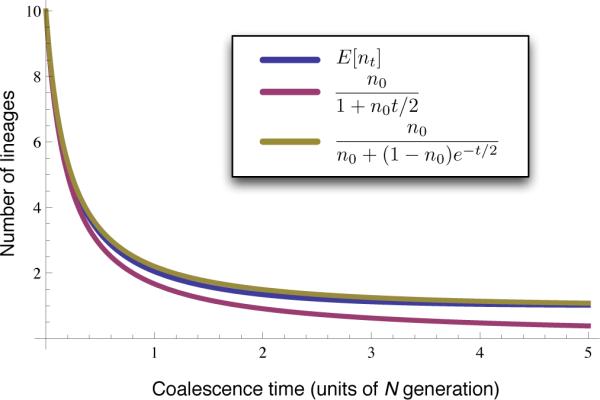
Comparision of simple approximations of E[n_t] in one population with n₀ = 10 sampled alleles. The exact mean E[n_t] (Equation 13, blue) is compared to the approximation of Slatkin and Rannala (1997) and Volz et al. (2009) (Equation 17, purple) and to the approximation of Frost and Volz (2010) and Maruvka et al. (2011) (Equation 18, green).

4.2. Approximating E[n_t] under migration

In this section, we extend the derivation of Slatkin and Rannala (1997) to the case of k populations, each of variable size N_i(z) (i = 1, ..., k) at time z ≥ 0 in the past, with migration among them. In the model we consider, lineages in population i migrate to population j at rate m_ij as time moves backward, where the m_ij represent backwards migration rates.

Let n_t = (n_1,t, n_2,t, ..., n_k,t) record the number of ancestral lineages in all populations at time t in the past. If the lineages follow a coalescent process in each population, n_t satisfies a time inhomogeneous Markov process with instantaneous transition probabilities given by

$$\mathbb{P}({\mathbf{n}}_{t+\delta }={\phi }^{\prime }\mid {\mathbf{n}}_t=\phi )=\{\begin{array}{cc}1-\sum _{i=1}^k\left(\begin{array}{c}\hfill {\phi }_i\hfill \\ \hfill 2\hfill \end{array}\right)\frac{1}{N_i\left(t\right)}\delta -\sum _{i=1}^k{\sum }_{\begin{array}{c}\hfill j=1\hfill \\ \hfill j\ne i\hfill \end{array}}^k{\phi }_i{m}_{ij}\delta +o\left(\delta \right)\hfill & \text{if}\phi ={\phi }^{\prime }\hfill \\ {\phi }_i{m}_{ij}\delta +o\left(\delta \right)\hfill & \text{if}\phi ={\phi }^{\prime }+{\mathbf{e}}_i-{\mathbf{e}}_j\hfill \\ \left(\begin{array}{c}\hfill {\phi }_i\hfill \\ \hfill 2\hfill \end{array}\right)\frac{1}{N_i\left(t\right)}\delta +o\left(\delta \right)\hfill & \text{if}\phi ={\phi }^{\prime }+{\mathbf{e}}_i\hfill \\ 0\hfill & \text{otherwise},\hfill \end{array}\phantom{\}}$$ (22)

where e_i is the ith standard basis vector in which element i is equal to one and all other elements are equal to zero. In Equation (22), the term $\left(\begin{array}{c}\hfill {\phi }_i\hfill \\ \hfill 2\hfill \end{array}\right)\frac{1}{N_i\left(t\right)}$ is the instantaneous rate at which a coalescent event occurs in population i, and φ_im_ij is the instantaneous rate at which a lineage migrates from population i to population j, when φ_i lineages remain in population i at time t. The notation φ′ = φ + e_i indicates that a coalescent event occurred in population i between the state φ at time t and the state φ′ at time t + δ . Equation (22) is the generalization of the transition probabilities used in the derivation of Volz et al. (2009, p.1880).

Using the transition probabilities in Equation (22) and conditioning on the state at time t, we obtain the following conditional expression for $\mathbb{P}({\mathbf{n}}_{t+\delta }=\phi )$, which we denote by p_φ(t + δ ):

$$p_{\phi }(t+\delta )=\left[1-\sum _{i=1}^k\left(\begin{array}{c}\hfill {\phi }_i\hfill \\ \hfill 2\hfill \end{array}\right)\frac{1}{N_{\ell }\left(t\right)}\delta -\sum _{i=1}^k\sum _{\begin{array}{c}\hfill j=1\hfill \\ \hfill j\ne i\hfill \end{array}}^k{\phi }_i{m}_{ij}\delta \right]p_{\phi }\left(t\right)+\sum _{i=1}^k\sum _{\begin{array}{c}\hfill j=1\hfill \\ \hfill j\ne i\hfill \end{array}}^k({\phi }_i+1)m_{ij}\delta p_{\phi +{\mathbf{e}}_i-{\mathbf{e}}_j}\left(t\right)+\sum _{i=1}^k\left(\begin{array}{c}\hfill {\phi }_i+1\hfill \\ \hfill 2\hfill \end{array}\right)\frac{1}{N_{\ell }\left(t\right)}\delta p_{\phi +{\mathbf{e}}_i}\left(t\right)+o\left(\delta \right).$$ (23)

Subtracting the term p_φ(t) from both sides, dividing by δ, and letting δ → 0 gives the differential equation

$$\frac{d{p}_{\phi }\left(t\right)}{dt}=-\sum _{i=1}^k\left(\begin{array}{c}\hfill {\phi }_i\hfill \\ \hfill 2\hfill \end{array}\right)\frac{1}{N_{\ell }\left(t\right)}{p}_{\phi }\left(t\right)-\sum _{i=1}^k\sum _{\begin{array}{c}\hfill j=1\hfill \\ \hfill j\ne i\hfill \end{array}}^k{\phi }_i{m}_{ij}{p}_{\phi }\left(t\right)+\sum _{i=1}^k\sum _{\begin{array}{c}\hfill j=1\hfill \\ \hfill j\ne i\hfill \end{array}}^k({\phi }_i+1)m_{ij}{p}_{\phi +{\mathbf{e}}_i-{\mathbf{e}}_j}\left(t\right)+\sum _{i=1}^k\left(\begin{array}{c}\hfill {\phi }_i+1\hfill \\ \hfill 2\hfill \end{array}\right)\frac{1}{N_{\ell }\left(t\right)}{p}_{\phi +{\mathbf{e}}_i}\left(t\right).$$ (24)

To obtain the differential equation for $E\left[n_{\ell t}\right](\ell =1,\dots ,k)$, we can multiply both sides of Equation (24) by ${\phi }_{\ell }$ and sum over ${\phi }_{\ell }$ (Appendix E) to obtain

$$\frac{dE\left[n_{\ell t}\right]}{dt}=-\left(\begin{array}{c}\hfill E\left[n_{\ell t}\right]\hfill \\ \hfill 2\hfill \end{array}\right)\frac{1}{N_{\ell }\left(t\right)}-\frac{\mathrm{Var}\left(n_{\ell t}\right)}{2N_{\ell }\left(t\right)}+\sum _{\begin{array}{c}\hfill i=1\hfill \\ \hfill i\ne \ell \hfill \end{array}}^k(m_{i\ell }E\left[n_{it}\right]-m_{\ell i}E\left[n_{\ell t}\right]).$$ (25)

If we assume that $\mathrm{Var}\left(n_{\ell t}\right)=0$, we obtain the system of k approximate differential equations

$$\frac{dE\left[n_{\ell t}\right]}{dt}\approx -\left(\begin{array}{c}\hfill E\left[n_{\ell t}\right]\hfill \\ \hfill 2\hfill \end{array}\right)\frac{1}{N_{\ell }\left(t\right)}+\sum _{\begin{array}{c}\hfill i=1\hfill \\ \hfill i\ne \ell \hfill \end{array}}^k(m_{i\ell }E\left[n_{it}\right]-m_{\ell i}E\left[n_{\ell t}\right]).$$ (26)

for $\ell =1,\dots ,k$, which can be solved numerically to obtain approximations of $E\left[n_{\ell t}\right]$.

The accuracy of the approximation obtained by solving the system of equations in Equation (26) is shown in Figure 4 for the case of two populations with migration among them. The populations have equal and exponentially growing sizes given by N₁(t) = N₂(t) = N(t), where N(t) satisfies the differential equation

$$N^{\prime }\left(t\right)=-\alpha N{\left(t\right)}^{\beta }.$$ (27)

This equation represents the model of super-exponential growth proposed by Reppell et al. (2012). When β = 1, the population size changes exponentially over time according to N(t) = N(0)e^{− t}. In the example in Figure 4, we have constrained the migration rates to be equal, and we consider the case in which n_1,0 = 100 lineages are sampled from the first population and n_2,0 = 0 lineages are sampled from the second population. From Figure 4, it can be seen that the approximation obtained by solving Equation (26) is accurate across a range of migration rates.

Figure 4.

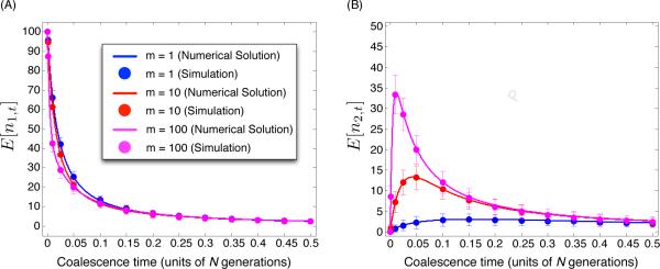
The accuracy of the approximation to E[n_t] under migration (Equation 26) for two populations of time-varying sizes N₁(t) and N₂(t). The two populations have the same size N₁(t) = N₂(t) = N(t), which grows faster-than-exponentially over time according to the formula dN(t)/dt = α− N(t)^β , where α = 10, β = 5, and N(0) = 1. The migration rates satisfy m₁₂ = m₂₁ = m. (A) Curves show the approximation of E[n_1,t] (the expected number of lineages in population 1 at time t) obtained by numerically solving Equation (26). Dots show the estimates of E[n_1,t] at the times t = 0.001, 0.01, 0.025, 0.05, 0.1, 0.15, 0.2, 0.25, 0.3, 0.35, 0.4, 0.45 and 0.5 obtained by simulating 10³ genealogies under the coalescent model according to the transition probabilities in Equation (22) and computing the number of lineages over this grid of times. different colored lines correspond to different values of m. The total length of each error bar is equal to two standard deviations of n_1,t or n_2,t, estimated from the 10³ replicate simulations (10³ sampled genealogies). (B) The corresponding plot for E[n_2,t], the expected number of lineages in population 2 at time t. For each value of m, n_1,0 = 100 and n_2,0 = 0 lineages were sampled from populations 1 and 2, respectively.

5. Applications

In this section, we apply the approximations in Equations (4), (7), and (10) to a set of example problems that demonstrate their utility for approximating coalescent formulas. We explore the accuracy of the resulting approximations using Theorems 2.1 and 3.1. We also demonstrate how approximations of E[n_t] for the case of multiple populations with migration (Equation 26) can be used to obtain approximate coalescent formulas under complicated demographic scenarios.

5.1. The expected joint allele frequency spectrum

We first consider the problem of approximating Wakeley and Hey's (1997) formula for the expected joint allele frequency spectrum between a pair of populations without migration. In Wakeley and Hey's model, two populations diverge at time t_D from an ancestral population (Figure 5). A sample of n_1,0 alleles is taken from the first population and a sample of n_2,0 alleles is taken from the second population. Let z_ij be the random variable recording the number of polymorphic sites for which the derived allele appears in i copies in the sample from the first population and in j copies in the sample from the second population. The expected joint allele frequency spectrum (JAFS) for the two populations is the collection of expectations E[z_ij] for i = 1, ..., n_1,0 − 1 and for j = 1, ..., n_2,0 − 1.

Figure 5.

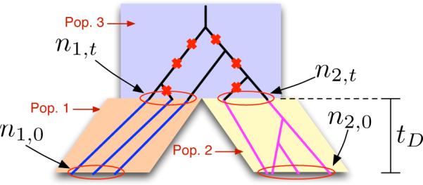
Wakeley and Hey's model for computing the expected joint allele frequency spectrum between a pair of populations. Two daughter populations, 1 and 2, diverge at time t_D in the past from an ancestral population (population 3). At the present time t = 0, n_1,0 and n_2,0 lineages are sampled from populations 1 and 2, respectively. Wakeley and Hey's formula for the expected joint allele frequency spectrum computes the expected number z_ij of segregating sites at which the derived allele appears in i copies in the sample from population 1 and in j copies in the sample from population 2, where i ∈ {1, ..., n_1,0} and j ∈ {1, ..., n_2,0}. The model considers only mutations that arose in the ancestral population (red crosses).

The expected JAFS is useful for performing inference on demographic parameters such as divergence times and ancestral population sizes (Wakeley and Hey 1997, Gutenkunst et al. 2009, Nielsen et al. 2009). Wakeley and Hey's formula for the expected JAFS is of the form

$$E\left[z_{ij}\right]=\sum _{n_{1,t_D}=2}^{n_{1,0}}\sum _{n_{2,t_D}=2}^{n_{2,0}}{C}_{ij}(n_{1,t_D},n_{2,t_D})\mathbb{P}\left(n_{1,t_D}\right)\mathbb{P}\left(n_{2,t_D}\right).$$ (28)

Here, t_D is the divergence time between the two populations, and

$$C_{ij}(n_{1,t_D},n_{2,t_D})=\sum _{k_1=1}^{n_{1,t_D}-1}\sum _{k_2=1}^{n_{2,t_D}-1}P(k_1\to i\mid n_{1,0},n_{1,t_D})P(k_2\to j\mid n_{2,0},n_{2,t_D})\frac{\left(\begin{array}{c}\hfill n_{1,t_D}\hfill \\ \hfill k_1\hfill \end{array}\right)\left(\begin{array}{c}\hfill n_{2,t_D}\hfill \\ \hfill k_2\hfill \end{array}\right)}{\left(\begin{array}{c}\hfill n_{1,t_D}+n_{2,t_D}\hfill \\ \hfill k_1+k_2\hfill \end{array}\right)}\frac{1}{k_1+k_2},$$ (29)

where $P(k\to i\mid n,n^{\prime })=\left(\begin{array}{c}\hfill n-n^{\prime }\hfill \\ \hfill i-k\hfill \end{array}\right)k_{(i-k)}{(n^{\prime }-k)}_{(n-n^{\prime }-i+k)}∕{n^{\prime }}_{(n-n^{\prime })}$.

The term C_ij(n_1,tD, n_2,tD) is time-consuming to evaluate, and the formula in Equation (28) quickly becomes computationally burdensome as n_1,0 and n_2,0 increase in size (Figure 6A). Dependence on the distribution $\mathbb{P}\left(n_{t_D}\right)$ also leads to round-off error when n_1,0 or n_2,0 is large and t_D is small. This round-off error is visible in Figure 6B as points that deviate from the smooth curve for sample sizes greater than n_1,0 = n_2,0 ≈ 60.

Figure 6.

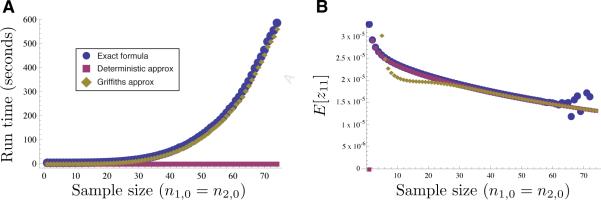
Three different approaches for computing the first term E[z₁₁] in the expected joint allele frequency spectrum between two populations for different numbers n_1,0 and n_2,0 of sampled alleles, with n_1,0 = n_2,0: Wake-ley and Hey's (1997) exact formula (Equation 28, blue), the deterministic approximation computed using Equation (4) (magenta), and Griffiths’ approximation computed using Equation (3) (green). (A) The running time is shown as a function of the sample sizes n_1,0 and n_2,0 in the two populations. (B) The value from each of three methods for computing the term E[z₁₁].

5.1.1. Approximating the JAFS

Although Griffiths’ approximation (Equation 3) can eliminate the round-off error in evaluating Equation (28), the time needed to compute the Griffiths approximation is nearly the same as the time needed to compute the exact formula (Figure 6A). In addition, the approximation deviates from the true value when the sample size is small (Figure 7A).

Figure 7.

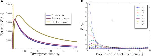
The error in approximating the expected joint allele frequency spectrum (JAFS). (A) The error in approximating the first term E[z₁₁] in the expected JAFS between two populations for the case of n_1,0 = n_2,0 = 30 sampled alleles for a range of divergence times t_D. The absolute value of the exact error in the deterministic approximation of Wakeley and Hey's (1997) formula for the expected JAFS (Equation 30, blue), the estimated error of the approximation in Equation (30) obtained using Equation (12) (magenta), and the error in Griffiths’ approximation obtained using Equation (3) (green) are shown. (B) Comparison of Wakeley and Hey's exact formula (Equation 28) with the deterministic approximation (Equation 30) for all possible combinations of allele counts i and j for the case of constant and equal sized populations (N₁ = N₂ = N₃ = N), for sample sizes n_1,0 = n_2,0 = 30, and for a divergence time of t_D = 0.01 coalescent units of N generations. The value of Wakeley and Hey's formula is shown with a solid line and the deterministic approximation is shown with dots.

Instead of using the Griffiths approximation, we can approximate Equation (28) using the deterministic approximation (Equation 4). In particular, we can approximate Equation (28) as

$$E\left[z_{ij}\right]\approx C_{ij}(E\left[n_{1,t_D}\right],E\left[n_{2,t_D}\right])$$ (30)

The expectations E[n_1,tD] and E[n_2,tD] in Equation (30) can be computed using Equation (13), or they can be approximated using Equation (17) or Equation (18). Because E[n_1,tD] and E[n_2,tD] are not generally integer-valued, the factorials and binomial coefficients in Equation (29) can be computed by reformulating them in terms of gamma functions using the definitions n! = Γ(n + 1) and $\left(\begin{array}{c}\hfill n\hfill \\ \hfill k\hfill \end{array}\right)=n!∕[k!(n-k)!]=\Gamma (n+1)∕\left[\Gamma (n-k+1)\right]$. The result of the approximation is a considerable reduction in computation time (Figure 5A) and a considerable improvement in accuracy both for small and for large sample sizes (Figure 5B).

5.1.2. The accuracy and computational complexity of the approximation in Equation (30)

Theorem 3.1 tells us that when the second partial derivatives ${\partial }_{n_{1,t_D}}^2{C}_{ij}(n_{1,t_D},n_{2,t_D})$ and ${\partial }_{n_{2,t_D}}^2{C}_{ij}(n_{1,t_D},n_{2,t_D})$ exist and are continuous and bounded in n_1,tD and n_2,tD, then the approximation in Equation (30) converges to the true distribution in Equation (28) as t → 0 and as t → ∞. Because Equation (29) is a finite sum of fractions of gamma functions in n_1,tD and n_2,tD, which are smooth, bounded, and nonzero for (n_1,tD, n_2,tD) ∈ [1, n_1,0] × [1, n_2,0], the second partial derivatives of Equation (29) are smooth and bounded on [1, n_1,0] × [1, n_2,0]. Therefore, for fixed values of n_1,0 and n_2,0, the error in the approximation in Equation (30) decreases to zero as t → 0 and as t → ∞.

We can also estimate the magnitude of the error in the deterministic approximation using the result in Appendix D. In particular, because the lineages in populations 1 and 2 coalesce independently of one another, we can estimate the error using Equation (12), which applies when n_1,t and n_2,t are independent. In Equation (12) the variances Var(n_1,tD) and Var(n_2,tD) can be computed using Tavaré's formula given in Equation (B.3). Because the second partial derivatives ${\partial }_{n_{1,t_D}}^2{C}_{ij}(n_{1,t_D},n_{2,t_D})$ and ${\partial }_{n_{2,t_D}}^2{C}_{ij}(n_{1,t_D},n_{2,t_D})$ are difficult to compute analytically, we can evaluate them using finite difference approximations; in this example, we used the second-order forward finite difference approximation.

The asymptotic accuracy of the approximation in Equation (30) can be seen in Figure 7A for the term E[z₁₁]. In particular, the blue curve, which corresponds to the error in the deterministic approximation, approaches zero as t → 0 and as t → ∞. From Figure 7A it can also be seen that the estimated error in the approximation to the term E[z₁₁] closely matches the true error, and that it is approximately equal to the true error in the limits t → 0 and t → ∞. The error is also small for the other terms in the JAFS. For example, for the fixed value t_D = 0.01 and for n_1,0 = n_2,0 = 30, the fit of the approximation in Equation (30) is very accurate for all values of i and j (Figure 7B).

In contrast with the deterministic approximation, the error in the Griffiths approximation (the green curve in Figure 7A) does not converge to zero as t → 0. Although the Griffiths approximation is less accurate than the deterministic approximation for the particular choice of parameter values considered here, the Griffiths approximation is guaranteed to converge to the exact value as t → 0 and as n_1,0 and n_2,0 increase to infinity. Thus, the accuracy of the Griffiths approximation will improve for larger sample sizes.

5.2. Expected numbers of segregating sites under migration

In this section, we demonstrate how approximate expected numbers of segregating sites can be computed under complicated demographic scenarios involving variable population sizes and migration. In particular, we combine Equation (10) with approximations of E[n_t] obtained using Equation (26) to compute the expected number of private alleles in a sample from a population. Private alleles are useful for studying the historical relationships among populations (Tishkoff and Kidd 2004, Szpiech et al. 2008), and the number of private alleles is a commonly-used measure of species uniqueness in conservation studies (e.g., Kalinowski 2004, Wilson et al. 2012, Ariani et al. 2013).

In this example, we again consider two populations, 1 and 2, that diverged at time t_D in the past and that have continued to share migrants since their divergence (Figure 8A). Let N₁(t) and N₂(t) be the sizes of populations 1 and 2 at time t in the past. We consider the case in which each population has grown faster-than-exponentially over time (Equation 27) according to $N_i^{\prime }\left(t\right)=\alpha N_i{\left(t\right)}^{\beta }(i=1,2)$, where α and β are the same for both populations. We assume that n_1,0 and n_2,0 alleles were sampled from populations 1 and 2, respectively (Figure 8).

Figure 8.

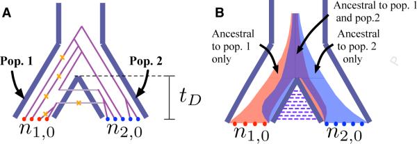
Comparison of stochastic and deterministic coalescent models for computing the expected number of mutations that are private to a sample of alleles from a population. In each model, two populations, 1 and 2, diverge at time t_D in the past. Samples of sizes n_1,0 and n_2,0 are taken from populations 1 and 2, respectively. (A) The classical stochastic coalescent model. Orange crosses indicate mutations that occur on lineages that are ancestral only to the sample from population 1. (B) The deterministic coalescent model. The red region indicates lineages ancestral only to the sample from population 1, the blue region indicates lineages ancestral only to the sample from population 2, and the purple region indicates lineages ancestral to both samples. The width of the shaded region of each color in each population at a fixed time t is the expected number of lineages of the given type in the given population at that time. The total sum of branch lengths on which a mutation ancestral only to the sample from population 1 can occur is the area of the region shaded in red.

5.2.1. Approximating the expected number of private segregating sites in a sample

Let S₁ be the number of mutations that are observed in a region of length b bases in a sample of n_1,0 lineages from population 1 and not in a sample of n_2,0 lineages from population 2. The expectation E[S₁] can be obtained by computing the total sum of lengths L₁ of genealogy branches that are ancestral only to the sample from population 1 (Figure 8B). Using Equations (9) and (10), E[S₁] can be computed as

$$E\left[S_1\right]=\frac{\theta b}{4}E\left[L_1\right]=\frac{\theta b}{4}{\int }_{z=0}^{\infty }E\left[{\tilde{n}}_{1,z}\right]dz,$$ (31)

whereñ_1,t is the number of lineages that are ancestral only to the sample from population 1 and that are not ancestral to the sample from population 2.

To compute E[ñ_1,t], we can solve Equation (26) for two populations with initial conditions in which n_1,0 and n_2,0 alleles are initially sampled from populations 1 and 2, respectively. The solution gives us E[n_1,t] and E[n_2,t], the numbers of ancestral lineages remaining in populations 1 and 2, respectively, at time t in the past. Solving the system again with initial conditions in which no alleles are sampled from population 1 and in which n_2,0 alleles are sampled from population 2 yields the solutions E[y_1,t] and E[y_2,t], which are the numbers of lineages in populations 1 and 2, respectively, that are ancestral at time t to the n_2,0 lineages sampled from population 2.

The number of lineages E[x̃_1,t] in population 1 at time t that are ancestral only to the sample from population 1, and not to the sample from population 2, is then given by E[x̃_1,t] = E[n_1,t] − E[y_1,t]. Similarly, the number of lineages E[x̃_2,t] in population 2 at time t that are ancestral only to the sample from population 1, and not to the sample from population 2, is given by E[x̃_2,t] = E[n_2,t] − E[y_2,t]. Thus, the expected total number of lineages ancestral only to the sample from population 1 is given by E[[notdef]_1,t] = E[x̃_1,t] + E[x̃_2,t]. The expectation E[S₁] is then obtained by plugging the value of E[ñ_1,t] into Equation (31) for a given choice of θ and b.

Theorem 2.1 implies that Equation (31) is exact if E[ñ_1,t] is exact. However, because the differential equation in Formula (26) is approximate, there will be a small amount of error in our computation of E[S₁]. We examine this error empirically in Section 5.2.2.

5.2.2. The accuracy of the approximation in Equation (31)

To examine the error in Equation (31) that arises from the approximation in Equation (26), we compared the analytical results obtained using Equations (26) and (31) to simulations. Simulations were performed by sampling genealogies from the Markov chain with transition probabilities given by Equation (22) using an approach similar to that described by Jewett et al. (2012). We discuss the simulation procedure in more detail in Appendix F.

Approximations of E[S₁] appear in Figure 9 for various sample sizes n_1,0 and n_2,0, along with simulated values for comparison. In our computations and simulations, we have taken N₁(0) = N₂(0) = 1, and we have set N₃(t) = N₁(t_D) + N₂(t_D) at the divergence time t_D. The other parameters were chosen in order to model moderate levels of faster-than-exponential growth and migration: α = 5, β = 10, and m₁₂ = m₂₁ = 10. Because the parameters b and θ in our model only affect the computed values of E[S₁] by a constant scaling factor, we set each of these values to unity for simplicity (b = 1 and θ = 1). From Figure 9, it can be seen that the approximation is very accurate over the range of parameter values, even when the sample sizes are small.

Figure 9.

Comparison with simulations of analytical approximations of E[S₁] obtained using Equation (31) with simulations.

5.3. The time to the first inter-sample coalescent event

In the examples in Sections 5.1 and 5.2, we have used the approximation n_t ≈ E[n_t] to compute expected values. However, the approximation can also be used to derive approximate probability distributions. For example, Volz et al. (2009) used a version of the approximation in Equation (4) to compute the joint distribution of coalescent waiting times among a set of sampled lineages in a single population of variable size (Volz et al. 2009, Eqn. 12). Here, we consider the related problem of computing the distribution of the time until the first coalescent event between two different sets of sampled alleles in a model with two populations of variable size with migration among them (Figure 10).

Figure 10.

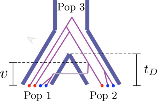
The time v until the first coalescent event occurs between an ancestor of one of n_1,0 type-1 alleles (red) and an ancestor of one of n_2,0 type-2 alleles (blue). The alleles are sampled from two populations, 1 and 2, of sizes N₁(t) and N₂(t) that diverged at time t_D from an ancestral population (population 3) of size N₃(t).

We again consider a model in which two populations diverge at time t_D from a common ancestral population (Figure 10). Consider a sample of n_1,0 alleles from one or both of the populations, and denote these as “type-1” alleles. Suppose that a second sample of n_2,0 alleles is taken from one or both populations and denote these as “type-2” alleles. We refer to lineages ancestral to type-1 alleles as “type-1” lineages, and we refer to lineages ancestral to the type-2 alleles as “type-2” lineages. We are interested in computing the distribution of the time V until the first coalescent event occurs between a type-1 lineage and a type-2 lineage when the migration rates between the populations are nonzero. We refer to a coalescent event between a type-1 lineage and a type-2 lineage as an inter-sample coalescent event.

Inter-sample coalescence times have a number of applications. For example, when the type-1 and type-2 alleles are each sampled from two different populations, the time to the first inter-sample coalescent event can be used to estimate the divergence time of the two populations (Takahata and Nei 1985, Mossel and Roch 2010, Liu et al. 2010, Jewett and Rosenberg 2012). When n_1,0 = 1, the distribution of the time to the first inter-sample coalescent event can be used to compute the probability of observing a new haplotype, conditional on an observed set of n_2,0 haplotypes (Paul and Song 2010), or to predict the accuracy of imputing genotypes on a haplotype using a reference panel of existing haplotypes (Jewett et al. 2012, Huang et al. 2013). The expected time of the first intersample coalescent event was computed using simulations by Takahata and Slatkin (1990). Here, we show how a simple approximate analytical distribution can be derived using Equation (26).

5.3.1. Approximating the distribution of the inter-sample coalescence time

At time t in the past, suppose that x_1,t type-1 lineages and y_1,t type-2 lineages remain in population 1 and suppose that x_2,t type-1 lineages and y_2,t type-2 lineages remain in population 2. Under the classical stochastic coalescent model, the instantaneous rate of coalescence between type-1 and type-2 lineages in population 1 is x_1,ty_1,t/N₁(t) and the instantaneous rate of coalescence among type-1 and type-2 lineages in population 2 is x_2,ty_2,t/N₂(t). Therefore, because lineages can only coalesce within the same population, the instantaneous rate of coalescence among type-1 and type-2 lineages overall is $x_{1,t}{y}_{1,t}∕N_1\left(t\right)+x_{2,t}{y}_{2,t}∕N_2\left(t\right)$.

Let x_1,[0,∞], x_2,[0,∞], y_1,[0,∞], and y_2,[0,∞] denote sample paths of the stochastic processes describing the numbers of ancestors of each type in the time interval [0, ∞], and denote the collection of these paths by x_[0,∞]. Conditional on the sample paths x_[0,∞] and on the event that no inter-sample coalescent event has occurred by time t, it follows that in the small time interval [t, t + δ], the probability that no inter-sample coalescent event occurs is

$$\begin{array}{cc}\hfill \mathbb{P}({\mathcal{I}}_{[t,t+\delta ]}\mid {\mathcal{I}}_{[0,t]},{\mathbf{x}}_{[0,\infty ]})\approx & 1-(x_{1,t}{y}_{1,t}∕N_1\left(t\right)+x_{2,t}{y}_{2,t}∕N_2\left(t\right))\delta \hfill \\ \hfill \approx & \exp \{-(x_{1,t}{y}_{1,t}∕N_1\left(t\right)+x_{2,t}{y}_{2,t}∕N_2\left(t\right))\delta \},\hfill \end{array}$$ (32)

where ${\mathcal{I}}_{[r,s]}$ is the event that no inter-sample coalescence occurs in the time interval [r, s]. Thus, conditional on the sample paths x_[0,∞], the probability that no inter-sample coalescent event occurs in any of v/δ small time intervals of length between time 0 and time v is given approximately by

$$\begin{array}{cc}\hfill \mathbb{P}({\mathcal{I}}_{[0,\delta ]},{\mathcal{I}}_{[\delta ,2\delta ]},\dots ,{\mathcal{I}}_{[v-\delta ,v]}\mid {\mathbf{x}}_{[0,\infty ]})\approx & \prod _{i=1}^{v∕\delta }{e}^{-(x_{1,i\delta }{y}_{1,i\delta }∕N_1\left(i\delta \right)+x_{2,i\delta }{y}_{2,i\delta }∕N_2\left(i\delta \right))\delta }\hfill \\ \hfill =& e^{-\sum _{i=1}^{v∕\delta }(x_{1,i\delta }{y}_{1,i\delta }∕N_1\left(i\delta \right)+x_{2,i\delta }{y}_{2,i\delta }∕N_2\left(i\delta \right))\delta }.\hfill \end{array}$$ (33)

A similar result was obtained for the case of a single population by Jewett and Rosenberg (2012).

By letting δ → 0 in Equation (33), we obtain an approximation of the survival function S_V|_x(v) of the time until the first inter-sample coalescent event, conditional on the sample paths x_[0,∞]:

$$\begin{array}{cc}\hfill S_{V\mid \mathbf{x}}\left(v\right)=& \mathbb{P}({\mathcal{I}}_{[0,v]}\mid {\mathbf{x}}_{[0,\infty ]})\hfill \\ \hfill \approx & e^{-{\int }_{z=0}^v}(x_{1,z}{y}_{1,z}∕N_1\left(z\right)+x_{2,z}{y}_{2,z}∕N_2\left(z\right))dz.\hfill \end{array}$$ (34)

The unconditional survival function S(v) can be obtained by integrating over all sample paths as follows:

$$\begin{array}{cc}\hfill S\left(v\right)=& {\int }_{{\mathcal{A}}_{[0,\infty ]}}{S}_{V\mid \mathbf{x}}\left(v\right)p\left({\mathbf{x}}_{[0,\infty ]}\right)d{\mathcal{A}}_{[0,\infty ]}\hfill \\ \hfill =& {\int }_{{\mathcal{A}}_{[0,\infty ]}}{e}^{-{\int }_{z=0}^v(x_{1,z}{y}_{1,z}∕N_1\left(z\right)+x_{2,z}{y}_{2,z}∕N_2\left(z\right))dz}p\left({\mathbf{x}}_{[0,\infty ]}\right)d{\mathcal{A}}_{[0,\infty ]},\hfill \end{array}$$ (35)

where p(x_[0,∞]) is the probability density function of the sample paths x_[0,∞]. Equation (35) is of the form given in Equation (5), which is time-consuming to compute due to the integral over all sample paths x_[0,∞]. However, using an approximation of the form given in Equation (7), we can approximate S(v) by

$$S\left(v\right)\approx e^{-{\int }_{z=0}^v(E\left[x_{1,z}\right]E\left[y_{1,z}\right]∕N_1\left(z\right)+E\left[x_{2,z}\right]E\left[y_{2,z}\right]∕N_2\left(z\right))dz}.$$ (36)

Compared with Equation (35), Equation (36) is considerably faster to compute and it has a simple functional form.

5.3.2. The accuracy of the approximation in Equation (36)

We compared the approximate distribution S(v) given in Equation (36) with kernel density estimates of S(v) from simulations (Appendix F). In our example, we considered a scenario in which the type-1 and type-2 lineages were sampled from different populations that diverged at time t_D = 0.1 and which had equal and faster-than-exponentially growing sizes given by N₁(t) = N₂(t). The population sizes N_i(t) (i = 1, 2) satisfied Equation (27) with N_i(0) = 1, β = 10, and α = 5. The ancestral population was of constant size N₃(t) = 1 for t ≥ t_D.

To obtain kernel density estimates of S(v), we simulated genealogies from a coalescent model with transition probabilities given by Equation (22) as described in Appendix F. Figure 11 shows comparisons of S(v) computed using Equation (36) with kernel densities computed from 10⁵ replicates for a variety of different sample sizes n_1,0 and n_2,0. From the density plots, it can be seen that the approximation is very accurate, even when the sample sizes are small.

Figure 11.

Kernel density estimates (dashed lines) and analytical approximations (solid lines) of the survival function S(v) of the time V to the first inter-sample coalescent event between two samples of lineages taken from two separate populations. Analytical approximations were computed using Equation (36). These values were generated using a model in which the type-1 and type-2 lineages were sampled from different populations (Figure 10) that diverged at time t_D = 0.1 and which had equal and faster-than-exponentially growing sizes given by N₁(t) = N₂(t) = N(t). The migration rates between the populations in the time interval [0, t_D] are m₁₂ = m₂₁ = 10. The population sizes N(t) satisfied Equation (27) with N(0) = 1, β = 10, and α = 5. The ancestral population was of constant size N₃(t) = 1 for t ≥ t_D. The sharp change in the slope of the curves at time v = 0.1 is due to the instantaneous transition from two populations to a single population at the divergence time t_D.

6. Discussion

In this paper, we have considered the accuracy and applications of the deterministic approximation n_t ≈ E[n_t] for deriving approximate coalescent distributions that are fast and numerically stable to compute. In particular, we identified ways in which the approximation n_t ≈ E[n_t] can be applied procedurally to reduce the computational complexity and numerical instability of coalescent formulas that involve conditional summations over all possible values of n_t, or that involve integrals over all possible sample paths n_[r,s] of the coalescent process describing the number of ancestral lineages in a given time interval [r, s].

We have considered two different kinds of approximation. In Sections 2 and 3, we considered the approximation of n_t by its expected value E[n_t]. In Section 4, we considered a second kind of approximation: approximate formulas for E[n_t]. The first approximation, of n_t by E[n_t], holds whenever the behavior of n_t is nearly deterministic. As we showed in Lemma B.1, this deterministic behavior occurs in the limit as t → 0 and as t → ∞. By contrast, the range of values over which any given approximation of E[n_t] is valid depends on the approximation that is used. For instance, in Figure 3, we saw that the approximate function in Equation (18) is sensible in the limit as t → 0 and as t → ∞, whereas the simpler approximation in Equation (17) is sensible only in the limit as t → 0.

To facilitate the application of these approximations in practice, we showed that approximate coalescent formulas of the form given in Equation (4) converge to their true values as t → 0 and as t → ∞ under simple assumptions. We also derived an approximate expression for the error in these deterministic approximations (Equation 11). This approximate expression for the error can be used in practice to evaluate when any given approximate formula of the form given in Equation (4) is accurate.

We obtained approximate formulas for E[n_t] in the case of multiple populations with time-varying sizes and migration among them (Equation 26). These approximations were produced by extending differential equations for E[n_t] derived for the case of a single panmictic population by Slatkin and Rannala (1997), Volz et al. (2009), and Maruvka et al. (2011). The approximations of E[n_t] that we obtained facilitate the derivation of approximate coalescent formulas under complicated demographic scenarios. For example, we showed how approximations of E[n_t] under migration could be used to approximate the expected number of mutations occurring along the branches of a genealogy (Section 5.2) or to compute an approximate distribution of coalescent waiting times (Section 5.3) in demographic models involving multiple populations with migration. Such applications of the approximation n_t ≈ E[n_t] are useful because deriving exact formulas for coalescent quantities under models with both migration and population size changes can be difficult.

We have described a number of problems to which the approximation n_t ≈ E[n_t] can be applied. However, we have focused on quantities that can be derived conditional on knowledge of the total number of ancestral lineages remaining at a given time t or over a given time interval [r, s]. Quantities that require knowledge of the topology of the coalescent tree relating the ancestral lineages, or of the number of lineages of a particular type, may be more difficult to derive. It is likely that the approximation n_t ≈ E[n_t] can be used to derive a variety of approximate distributions beyond those discussed here; however, the approximation n_t ≈ E[n_t] must be applied in a new way for each new class of problem, and the theoretical accuracy of these applications must be evaluated anew.

One common use of the approximation n_t ≈ E[n_t] that we did not consider in this paper is the inference of the size of a population at each time in the past by fitting the observed values of n_t obtained from a reconstructed genealogy of a set of sampled alleles to the expected values E[n_t] (t ≥ 0) under a given demographic history (Frost and Volz 2010, Maruvka et al. 2011). The theoretical accuracy of such fitting approaches is difficult to determine analytically and remains a subject for further work.

The importance of coalescent approximations has been a subject of much recent interest, as it has become increasingly recognized that exact formulas or algorithms can be intractable in practical scenarios. Many recent studies have made use of a variety of simplifying assumptions and approximations to the coalescent, and to coalescent-like problems (Li and Stephens 2003, McVean and Cardin 2005, Marjoram and Wall 2006, Davison et al. 2009, Paul and Song 2010, RoyChoudhury 2011, Li and Durbin 2011, Sheehan et al. 2013). Our results on the approximation n_t ≈ E[n_t] contribute to this growing toolbox of coalescent-based approximations that can be used to derive functionally simple, computationally efficient, and numerically stable approximations of coalescent formulas under a variety of coalescent models. These, and similar kinds of approximations, will become increasingly important for making population-genetic computations tractable as the sizes of genomic data sets continue to grow.

Appendix A Proof of Theorem 2.1

Proof. Let $([r,s],\mathcal{L},\lambda )$ denote the measure space defined on the interval [r, s] with the Lebesgue σ-algebra on [r, s] and Lebesgue measure λ. Let ${\mathcal{A}}_{[r,s]}$ denote the space of sample paths n_[r,s] of the stochastic process n_t over the time interval [r, s], and define the measure space $({\mathcal{A}}_{[r,s]},S,p)$ where S is the σ-algebra generated by the process n_t and p is the probability distribution of sample paths on ${\mathcal{A}}_{[r,s]}$. We assume that $({\mathcal{A}}_{[r,s]},S,p)$ is complete, or if not, we assume that it is equal to its completion, which exists by the Completion Theorem (Rudin 1975, p.29). We have

$$E\left[L_{[r,s]}\right]=E\left[{\int }_{z=r}^s{n}_z{d}_z\right]={\int }_{{\mathcal{A}}_{[r,s]}}{\int }_{z=r}^z{n}_{z}p\left(n_{[r,s]}\right)dzd{\mathcal{A}}_{[r,s]}.$$ (A.1)

Tonelli's theorem (DiBenedetto 2002, Theorem 14.2, p.148) states that the integrals on the right-hand side of Equation (A.1) can be exchanged if $([r,s]\mathcal{L},\lambda )$ and $({\mathcal{A}}_{[r,s]},S,p)$ are complete σ-finite measure spaces and if n_zp(n_[r,s]) is a nonnegative measurable function on $[r,s]\times {\mathcal{A}}_{[r,s]}$. The function n_z is a positive step function on [r, s] and it is therefore measurable because a measurable function can be defined as a limit of step functions (Atkinson and Han 2009, p.17). The density function p(n_[r,s]) is also positive and measurable because probability density functions are positive and measurable by definition (Tao 2011, p.193). Therefore, the product n_zp(n_[r,s]) is positive and it is measurable because the product of measurable functions is measurable (Franks 2009, Page 48, Exercise 3.1.11). The space $([r,s],\mathcal{L},\lambda )$ is complete because the Lebesgue σ-algebra combined with the Lebesgue measure on a subset of the real numbers forms a complete measure space (Mas-Colell 1989, p.23), and $({\mathcal{A}}_{[r,s]},S,p)$ is complete by assumption. Because λ ([r, s]) = s − r < ∞ and $p\left({\mathcal{A}}_{[r,s]}\right)=1<\infty$, the measure spaces $([r,s],\mathcal{L},\lambda )$ and $({\mathcal{A}}_{[r,s]},S,p)$ are both sets of finite measure, and are therefore σ-finite by definition (DiBenedetto 2002, p.71). Therefore, it follows that the integrals in Equation (A.1) can be exchanged by Tonelli's Theorem, yielding

$$\begin{array}{cc}\hfill E\left[L_{[r,s]}\right]=& {\int }_{{\mathcal{A}}_{[r,s]}}{\int }_{z=r}^s{n}_{z}p\left(n_{[r,s]}\right)dzd{\mathcal{A}}_{[r,s]}\hfill \\ \hfill & {\int }_{z=r}^s{\int }_{{\mathcal{A}}_{[r,s]}}{n}_{z}p\left(n_{[r,s]}\right)d{\mathcal{A}}_{[r,s]}dz\hfill \\ \hfill =& {\int }_{z=r}^{s}E\left[n_z\right]dz,\hfill \end{array}$$ (A.2)

which completes the proof.

Appendix B. A lemma for proving Theorem 3.1

In this section we present a lemma that is necessary for proving Theorem 3.1. The lemma states that the number of lineages n_t that are ancestral to a set of n₀ sampled lineages approaches its expected value E[n_t] as t → 0 and as t → ∞. Specifically, we show that the random variable n_t − E[n_t] converges in probability to 0 as t → 0 and as t → ∞. We first show that Var(n_t) → 0 as t → 0 and as t → ∞ for fixed n₀ in a population of arbitrary size N(t).

Lemma B.1. Consider a panmictic population of variable size N(t) such that ${\lim }_{t\to 0}{\int }_{z=0}^t\frac{1}{N\left(s\right)}dz=0$ and ${\lim }_{t\to \infty }{\int }_{z=0}^t\frac{1}{N\left(z\right)}dz=\infty$. For a fixed number, n₀, of lineages sampled at time t = 0 from this population, Var(n_t) → 0 as t → 0 and as t → ∞.

Proof. Tavaré (1984, p.131) showed that the moments of n_t in a panmictic population of constant effective size N can be obtained using the function

$$E\left[{\left(n_t\right)}_{\left[k\right]}\right]=\sum _{i=k}^{n_0}(2i-1)\left(\begin{array}{c}\hfill i-1\hfill \\ \hfill k-1\hfill \end{array}\right)\frac{i_{(k-1)}{\left(n_0\right)}_{\left[i\right]}}{{\left(n_0\right)}_{\left(i\right)}}{e}^{-i(i-1)t∕2},$$ (B.1)

where E[(n_t)_[k]|n₀] is the kth factorial moment of $n_t,n_{\left[i\right]}=n!∕(n-i)$ and $n_{\left(i\right)}=(n-1+i)!∕(n-1)!$, and where time t is in coalescent units of N generations.

Chen and Chen (2013) noted that this formula can be extended to the case of a population of variable size N(t) using a result from Griffiths and Tavaré (1994). Specifically, Griffiths and Tavaré showed that in a population of variable size N(t), n_t has the same distribution as the number n _(t of ancestral lineages at time $\tau \left(t\right)={\int }_{z=0}^t\frac{1}{N\left(z\right)}dz$ in a population of constant size one. Thus, in a population of variable size N(t), Equation (B.1) becomes

$$E\left[{\left(n_t\right)}_{\left[k\right]}\right]=\sum _{i=k}^{n_0}(2i-1)\left(\begin{array}{c}\hfill i-1\hfill \\ \hfill k-1\hfill \end{array}\right)\frac{i_{(k-1)}{\left(n_0\right)}_{\left[i\right]}}{{\left(n_0\right)}_{\left(i\right)}}{e}^{-i(i-1)\tau \left(t\right)∕2},$$ (B.2)

where $\tau \left(t\right)={\int }_{z=0}^t\frac{1}{N\left(z\right)}dz$, and where t is in units of generations.

Using the definitions ${\left(n_t\right)}_{\left[2\right]}=n_t^2-n_t$ and (n_t)_[1] = n_t we can write

$$\mathrm{Var}\left(n_t\right)=E\left[n_t^2\right]-E{\left[n_t\right]}^2=E\left[{\left(n_t\right)}_{\left[2\right]}\right]+E\left[{\left(n_t\right)}_{\left[1\right]}\right]-E{\left[{\left(n_t\right)}_{\left[1\right]}\right]}^2,$$ (B.3)

where, from Equation (B.1), we have

$$E\left[{\left(n_t\right)}_{\left[2\right]}\right]=\sum _{i=2}^{n_0}(2i-1)(i-1)\frac{i{\left(n_0\right)}_{\left[i\right]}}{{\left(n_0\right)}_{\left(i\right)}}{e}^{-\left(\begin{array}{c}\hfill i\hfill \\ \hfill 2\hfill \end{array}\right)\tau \left(t\right)}$$ (B.4)

and

$$E\left[{\left(n_t\right)}_{\left[1\right]}\right]=\sum _{i=2}^{n_0}(2i-1)\frac{{\left(n_0\right)}_{\left[i\right]}}{{\left(n_0\right)}_{\left(i\right)}}{e}^{-\left(\begin{array}{c}\hfill i\hfill \\ \hfill 2\hfill \end{array}\right)\tau \left(t\right)}.$$ (B.5)

By assumption, we have τ(t) → ∞ as t → ∞. Since e⁻ → 0 as τ(t) → ∞ for i ≥ 2, it follows from Equation (B.4) that E[(n_t)_[2]] → 0 as t → ∞. Similarly, since n_[1] = n₍₁₎, Equation (B.5) yields

$$E\left[{\left(n_t\right)}_{\left[1\right]}\right]=1+\sum _{i=2}^{n_0}(2i-1)\frac{{\left(n_0\right)}_{\left[i\right]}}{{\left(n_0\right)}_{\left(i\right)}}{e}^{-\left(\begin{array}{c}\hfill i\hfill \\ \hfill 2\hfill \end{array}\right)\tau \left(t\right)}=1+\mathcal{O}\left(e^{-\tau \left(t\right)}\right),$$ (B.6)

from which it follows that E[(n_t)_[1]|n₀] → 1 as t → ∞. Thus, Var(n_t) → 0 as t → ∞ by plugging the limiting values of Equations (B.4) and (B.5) into the right-hand side of Equation (B.3).

To obtain the limiting behavior of Var(n_t) as t → 0, we can use the fact that $e^{-\left(\begin{array}{c}\hfill i\hfill \\ \hfill 2\hfill \end{array}\right)\tau \left(t\right)}=1-\left(\begin{array}{c}\hfill i\hfill \\ \hfill 2\hfill \end{array}\right)\tau \left(t\right)+\mathcal{O}\left(\tau {\left(t\right)}^2\right)$. Thus, from Equation (B.4), we have

$$\begin{array}{cc}\hfill E\left[{\left(n_t\right)}_{\left[2\right]}\right]& =\sum _{i=2}^{n_0}(2i-1)(i-1)\frac{i{\left(n_0\right)}_{\left[i\right]}}{{\left(n_0\right)}_{\left(i\right)}}\left[1-\left(\begin{array}{c}\hfill i\hfill \\ \hfill 2\hfill \end{array}\right)\tau \left(t\right)+\mathcal{O}\left(\tau {\left(t\right)}^2\right)\right]\hfill \\ \hfill & =\sum _{i=2}^{n_0}(2i-1)(i-1)\frac{i{\left(n_0\right)}_{\left[i\right]}}{{\left(n_0\right)}_{\left(i\right)}}-\tau \left(t\right)\sum _{i=2}^{n_0}(2i-1)(i-1)\frac{i{\left(n_0\right)}_{\left[i\right]}}{{\left(n_0\right)}_{\left(i\right)}}\left(\begin{array}{c}\hfill i\hfill \\ \hfill 2\hfill \end{array}\right)+\mathcal{O}\left(\tau {\left(t\right)}^2\right)\hfill \\ \hfill & ={n_0}^2-n_0-\tau \left(t\right)\sum _{i=2}^{n_0}(2i-1)i(i-1)\frac{{\left(n_0\right)}_{\left[i\right]}}{{\left(n_0\right)}_{\left(i\right)}}\left(\begin{array}{c}\hfill i\hfill \\ \hfill 2\hfill \end{array}\right)+\mathcal{O}\left(\tau {\left(t\right)}^2\right),\hfill \end{array}$$ (B.7)

where the three terms in the second equality correspond to the three terms in brackets in the first equality. The first term, $n_0^2-n_0$, in the third equality is obtained by noting that the first term in the second equality is equal to $E\left[{\left(n_0\right)}_{\left[2\right]}\right]=n_0^2-n_0$ (Equation B.4).

Similarly, from Equation (B.5) we have

$$\begin{array}{cc}\hfill E\left[{\left(n_t\right)}_{\left[1\right]}\right]& =\sum _{i=1}^{n_0}(2i-1)\frac{{\left(n_0\right)}_{\left[i\right]}}{{\left(n_0\right)}_{\left(i\right)}}\left[1-\left(\begin{array}{c}\hfill i\hfill \\ \hfill 2\hfill \end{array}\right)\tau \left(t\right)+\mathcal{O}\left(\tau {\left(t\right)}^2\right)\right]\hfill \\ \hfill & =n_0-\tau \left(t\right)\sum _{i=1}^{n_0}(2i-1)\frac{{\left(n_0\right)}_{\left[i\right]}}{{\left(n_0\right)}_{\left(i\right)}}\left(\begin{array}{c}\hfill i\hfill \\ \hfill 2\hfill \end{array}\right)+\mathcal{O}\left(\tau {\left(t\right)}^2\right)\hfill \\ \hfill & =n_0-\tau \left(t\right)\left(\begin{array}{c}\hfill n_0\hfill \\ \hfill 2\hfill \end{array}\right)+\mathcal{O}\left(\tau {\left(t\right)}^2\right),\hfill \end{array}$$ (B.8)

where the third equality is obtained by noting that the second term in the second equality is equal to half the expression for E[(n_t)_[2]] evaluated at time t = 0; it is therefore equal to $\left(\begin{array}{c}\hfill n_0\hfill \\ \hfill 2\hfill \end{array}\right)$. Squaring Equation (B.8) gives

$$E{\left[{\left(n_t\right)}_{\left[1\right]}\right]}^2=n_0^2-2n_0\tau \left(t\right)\left(\begin{array}{c}\hfill n_0\hfill \\ \hfill 2\hfill \end{array}\right)+\mathcal{O}\left(\tau {\left(t\right)}^2\right).$$ (B.9)

Thus, by plugging Equations (B.7), (B.8), and (B.9) into Equation (B.3), we obtain

$$\mathrm{Var}\left(n_t\right)=n_0^2-n_0+\mathcal{O}\left(\tau \left(t\right)\right)+n_0+\mathcal{O}\left(\tau \left(t\right)\right)-n_0^2+\mathcal{O}\left(\tau \left(t\right)\right)=\mathcal{O}\left(\tau \left(t\right)\right).$$ (B.10)

Here, we have used the fact that $\tau {\left(t\right)}^2=\mathcal{O}\left(\tau \left(t\right)\right)$. The right-hand side of Equation (B.10) follows from the linearity of order notation (Miller 2006, p.21). Thus, it follows from our assumption that N(t) varies in such a way that τ(t) → 0 as t → 0 that Var(n_t) → 0 as t → 0 for fixed values of n₀.

We now show that n_t − E[n_t] converges in probability to 0 as t → 0 and as t → ∞.

Lemma B.2. Consider a panmictic population of variable size N(t) at time t, such that ${\lim }_{t\to 0}{\int }_{z=0}^t\frac{1}{N\left(z\right)}dz=0$ and ${\lim }_{t\to \infty }{\int }_{z=0}^t\frac{1}{N\left(z\right)}dz=\infty$. Suppose that n₀ lineages are sampled from this population and consider the number of ancestral lineages n_t at time t in the past. Under the coalescent model, the random variable n_t − E[n_t] converges in probability to 0 as t → 0 and as t → ∞.

Proof. The quantity n_t is bounded above by n₀ and below by unity. Thus, n_t has finite mean and variance and therefore satisfies Chebyshev's inequality (Ross 2007, p.77). In particular, for any ε > 0, direct application of Chebyshev's inequality gives

$$\mathrm{Pr}(\mid n_t-E\left[n_t\right]\mid >∊)\le \frac{\mathrm{Var}\left(n_t\right)}{{∊}^2}.$$ (B.11)

In Lemma B.1 we showed that for fixed n₀, Var(n_t) → 0 as t → 0 and as t → ∞. By the sandwich theorem applied to Equation (B.11), it follows that, Pr(|n_t − E[n_t]| > ε) → 0 as t → 0 and as t → ∞. Thus, by the definition of convergence in probability (Casella and Berger 2002, p.232), n_t − E[n_t] converges in probability to 0.

Appendix C Proof of Theorem 3.1

Here, we prove that the deterministic approximation (Equation 4) is accurate as t → 0 and as t → ∞ for fixed n₀.

Proof. To prove Theorem 3.1, we can expand f(x|n_t) around the point E[n_t]. The first term in this expansion is simply our approximation f(x|E[n_t]), and we can show that the higher-order terms in the expansion converge to zero as t → 0 and as t → ∞.

By the second-order mean value theorem (Hendrix and Tóth 2010, p. 41), we have

$$f(x\mid {\mathbf{n}}_t)=f(x\mid E\left[{\mathbf{n}}_t\right])+{\nabla }_{{\mathbf{n}}_t}f(x\mid E\left[{\mathbf{n}}_t\right])({\mathbf{n}}_t-E\left[{\mathbf{n}}_t\right])+{({\mathbf{n}}_t-E\left[{\mathbf{n}}_t\right])}^T\frac{1}{2}{H}_{{\mathbf{n}}_t}\left[f(x\mid {\mathbf{c}}_t)\right]({\mathbf{n}}_t-E\left[{\mathbf{n}}_t\right]),$$ (C.1)

Where H_nt [f(x|c_t)] is the Hessian of f(x|n_t) with respect to n_t evalutated at a point c_t given by c_t = E[n_t] + q(n_t − E[n_t]) for some q ∈ [0, 1]. Taking the expectation of both sides with respect to n_t and noting that f(x) = Σ_nt f(x|n_t) Pr(n_t) = E[f(x|n_t)], we obtain

$$f\left(x\right)=E\left[f(x\mid {\mathbf{n}}_t)\right]=f(x\mid E\left[{\mathbf{n}}_t\right])+\frac{1}{2}E\left[{({\mathbf{n}}_t-E\left[{\mathbf{n}}_t\right])}^T{H}_{{\mathbf{n}}_t}\left[f(x\mid {\mathbf{c}}_t)\right](n_t-E\left[{\mathbf{n}}_t\right])\right],$$ (C.2)

where the expectation of the second term in Equation (C.1) is equal to zero because E[n_t − E[n_t]] = 0. Rearranging Equation (C.2) and taking absolute values gives

$$\begin{array}{cc}\hfill \mid f\left(x\right)-f(x\mid E\left[{\mathbf{n}}_t\right])\mid =& \mid E\left[\frac{1}{2}{({\mathbf{n}}_t-E\left[{\mathbf{n}}_t\right])}^T{H}_{{\mathbf{n}}_t}\left[f(x\mid {\mathbf{c}}_t)\right]({\mathbf{n}}_t-E\left[{\mathbf{n}}_t\right])\right]\mid \hfill \\ \hfill =& \mid E\left[\frac{1}{2}\sum _{i=1}^k\sum _{j=1}^k(n_{i,t}-E\left[n_{i,t}\right])(n_{j,t}-E\left[n_{j,t}\right])\frac{{\partial }^2}{\partial n_{i,t}\partial n_{j,t}}f(x\mid {\mathbf{c}}_t)\right]\mid .\hfill \end{array}$$ (C.3)

To prove that f(x|E[n_t]) converges uniformly to f(x) on D as t → 0 and as t → ∞, we can bound the right-hand side of Equation (C.3) and show that this bounded quantity goes to zero as t → 0 and as t → ∞ for all x ∈ D. From Equation (C.3), we have

$$\begin{array}{cc}\hfill \mid f\left(x\right)-f(x\mid E\left[{\mathbf{n}}_t\right])\mid & \le \frac{1}{2}E\left[\frac{1}{2}\sum _{i=1}^k\sum _{j=1}^k\mid (n_{i,t}-E\left[n_{i,t}\right])(n_{j,t}-E\left[n_{j,t}\right])\mid \mid \frac{{\partial }^2}{\partial n_{i,t}\partial n_{j,t}}f(x\mid {\mathbf{c}}_t)\mid \right]\hfill \\ \hfill & \le M\sum _{i=1}^k\sum _{j=1}^{k}E\left[\mid (n_{i,t}-E\left[n_{i,t}\right])(n_{j,t}-E\left[n_{j,t}\right])\mid \right].\hfill \end{array}$$ (C.4)

Here, $M={\max }_{i,j\in \{1,\dots ,k\}}{\sup }_{c\in \mathcal{N}}\frac{1}{2}\mid \frac{{\partial }^2}{\partial n_{i,t},\partial n_{j,t}}f(x\mid c)$ exists on $D\times \mathcal{N}$ because we have assumed that the second-order partial derivatives $\frac{{\partial }^2}{\partial n_{i,t},\partial n_{j,t}}f(x\mid {\mathbf{n}}_t)$ are bounded. Considering the summand on the right-hand side of Equation (C.4), we have

$$E\left[\mid (n_{i,t}-E\left[n_{i,t}\right])(n_{j,t}-E\left[n_{j,t}\right])\mid \right]\le E\left[\mid n_{i,t}-E\left[n_{i,t}\right]\mid \mid n_{j,t}-E\left[n_{j,t}\right]\mid \right]\le n_{i,0}E\left[\mid n_{j,t}-E\left[n_{j,t}\right]\mid \right],$$ (C.5)

because |n_i,t−E[n_i,t]| ≤ n_i,0. Now, to show that the term on the right-hand side in Equation (C.5) converges to 0 as t → 0 and as t → ∞, we can use a convergence theorem from Van der Vaart (2000, Thm. 2.20). This theorem states that if a sequence W_n of random variables converges in probability to W in the limit as n → ∞, then E[W_n] → E[W ] as n → ∞, whenever W_n is asymptotically uniformly integrable. Thus, in Equation (C.5), E[|n_j,t − E[n_j,t]|] → E[0] = 0 if |n_i,t − E[n_i,t]| is asymptotically uniformly integrable.

A sequence of random variables W_n is asymptotically uniformly integrable (Van der Vaart 2000, p.17) if

$$\underset{M\to \infty }{\lim }\underset{n\to \infty }{\lim \sup }E\left[\mid W_n\mid 1_{\{\mid W_n\mid >M\}}\right]=0,$$ (C.6)

where 1_{|Wn|>M} is the indicator random variable with 1_{|Wn|>M} = 1 if |W_n| > M and 1_{|Wn|>M} = 0, otherwise. From this definition, it can be seen that |n_j,t − E[n_j,t]| is asymptotically uniformly integrable because E[|n_j,t−E[n_j,t]|1_{|nj,t−E[nj,t]|>M}] = 0 whenever M > sup |n_j,t − E[n_j,t]| = n_j,0. Therefore, the right-hand side of Equation (C.5) converges to zero as t → 0 and as t → ∞ for all x ∈ D and for fixed ${\mathbf{n}}_0\in \mathcal{N}$. By the sandwich theorem, it follows that E[|(n_i,t − E[n_i,t])(n_j,t − E[n_j,t])|] → 0 as t → 0 and as t → ∞. From a second application of the sandwich theorem, it follows that the left-hand-side of Equation (C.4), |f(x) − f(x|E[n_t])|, converges uniformly to 0 for all x in D as t → 0 and as t → ∞.

Appendix D Approximate error in the deterministic approximation

Equation (C.3) in the proof of Theorem 3.1 allows us to obtain an estimate of the error | f(x) − f(x|E[n_t])| in the deterministic approximation f(x) ≈ f(x|E[n_t]). From Equation (C.3), we have

$$\mid f\left(x\right)-f(x\mid E\left[{\mathbf{n}}_t\right])\mid =\mid \frac{1}{2}\sum _{i=1}^k\sum _{j=1}^{k}E\left[(n_{i,t}-E\left[n_{i,t}\right])(n_{j,t}-E\left[n_{j,t}\right])\frac{{\partial }^2}{\partial n_{i,t}\partial n_{j,t}}f(x\mid {\mathbf{c}}_t)\right]\mid .$$ (D.1)

Now, we showed in Lemma B.2 that n_i,t − E[n_i,t] converges in probability to 0 as t → 0 and as t → ∞. It follows that $\mathbb{P}(\Vert {\mathbf{n}}_t-E\left[{\mathbf{n}}_t\right]\Vert >∊)\to 0$ for any ε > 0 as t → 0 and as t → ∞. Thus, recalling that c_t = E[n_t] + q(n_t − E[n_t]), we have $\mathbb{P}(\Vert {\mathbf{c}}_t-E\left[{\mathbf{n}}_t\right]]\Vert >∊)=\mathbb{P}(\Vert {\mathbf{n}}_t-E\left[{\mathbf{n}}_t\right]]\Vert >∊∕q)\to 0$ as t → 0 and as t → ∞. Therefore, as t → 0 and as t → ∞, we can make the approximation c_t ≈ E[n_t]. Using the approximation c_t ≈ E[n_t] as t → 0 and as t → ∞, and approximating the expectation of a product by the product of the expectations, we obtain

$$\begin{array}{cc}\hfill \mid f\left(x\right)-f(x\mid E\left[{\mathbf{n}}_t\right])\mid \approx & \mid \frac{1}{2}\sum _{i=1}^k\sum _{j=1}^{k}E\left[(n_{i,t}-E\left[n_{i,t}\right])(n_{j,t}-E\left[n_{j,t}\right])\right]\left[\frac{{\partial }^2}{\partial n_{i,t}\partial n_{j,t}}f(x\mid E\left[{\mathbf{n}}_t\right])\right]\mid \hfill \\ \hfill =& \mid \frac{1}{2}\sum _{i=1}^k\sum _{j=1}^k\mathrm{Cov}(n_{i,t},n_{j,t})\frac{{\partial }^2}{\partial n_{i,t}\partial n_{j,t}}f(x\mid E\left[{\mathbf{n}}_t\right])\mid .\hfill \end{array}$$ (D.2)

Appendix E Details of the derivation of Equation (25)

To obtain Equation (25), we multiply both sides of Equation (24) by ${\phi }_{\ell }$ and sum over all ${\prod }_{i=1}^k{n}_{i,0}$ possible values of φ. We allow the summation over each index φ_i (i = 1, ... , k) to run from − ∞ to ∞:

$$\begin{array}{cc}\hfill \frac{dE\left[n_{\ell t}\right]}{dt}& =\frac{d}{dt}\sum _{\phi }{\phi }_{\ell }{p}_{\phi }\left(t\right)\hfill \\ \hfill & =-\sum _{i=1}^k\sum _{\phi }{\phi }_{\ell }\left(\begin{array}{c}\hfill {\phi }_i\hfill \\ \hfill 2\hfill \end{array}\right)\frac{1}{N_{\ell }\left(t\right)}{p}_{\ell }\left(t\right)-\sum _{i=1}^k\sum _{\begin{array}{c}\hfill j=1\hfill \\ \hfill j\ne i\hfill \end{array}}^k\sum _{\phi }{\phi }_{\ell }{\phi }_i{m}_{ij}{p}_{\phi }\left(t\right)+\sum _{i=1}^k\sum _{\begin{array}{c}\hfill j=1\hfill \\ \hfill j\ne i\hfill \end{array}}^k\sum _{\phi }{\phi }_{\ell }({\phi }_{\ell }+1)m_{ij}{p}_{\phi +{\mathbf{e}}_i-{\mathbf{e}}_j}\left(t\right)+\sum _{i=1}^k\sum _{\phi }{\phi }_{\ell }\left(\begin{array}{c}\hfill {\phi }_i+1\hfill \\ \hfill 2\hfill \end{array}\right)\frac{1}{N_{\ell }\left(t\right)}{p}_{\phi +{\mathbf{e}}_i}\left(t\right).\hfill \end{array}$$ (E.1)

Each term in Equation (E.1) can be separated into cases: cases in which $\ell \ne i,j$, or $\ell =i$ and $\ell \ne j$, or $\ell =j$ and $\ell \ne i$. The first and last terms on the right-hand side of Equation (E.1) separate into two terms each (corresponding to the cases $\ell =i$ and $\ell \ne i$), and the middle terms on the right-hand side of Equation (E.1) separate into three terms each (corresponding to the cases $\ell =i$, $\ell =j$, and $\ell \ne i,j$). Each of these terms can be further simplified by noting that summations over indices ${\phi }_h(h\ne \ell ,i)$ are summations over the marginal densities and result in factors of one. Thus, we obtain

$$\begin{array}{cc}\hfill \frac{dE\left[n_{\ell t}\right]}{dt}=& -\sum _{\begin{array}{c}\hfill i=1\hfill \\ \hfill i\ne \ell \hfill \end{array}}^k\sum _{{\phi }_{\ell }}\sum _{{\phi }_i}{\phi }_{\ell }\left(\begin{array}{c}\hfill {\phi }_i\hfill \\ \hfill 2\hfill \end{array}\right)\frac{1}{N_{\ell }\left(t\right)}{p}_{{\phi }_{\ell },{\phi }_i}\left(t\right)-\sum _{{\phi }_{\ell }}{\phi }_{\ell }\left(\begin{array}{c}\hfill {\phi }_{\ell }\hfill \\ \hfill 2\hfill \end{array}\right)\frac{1}{N_{\ell }\left(t\right)}{p}_{{\phi }_{\ell }}\left(t\right)\hfill \\ \hfill & -\sum _{\begin{array}{c}\hfill i=1\hfill \\ \hfill i\ne \ell \hfill \end{array}}^k\sum _{\begin{array}{c}\hfill i=1\hfill \\ \hfill j\ne i,\ell \hfill \end{array}}^k\sum _{{\phi }_{\ell }}\sum _{{\phi }_i}{\phi }_{\ell }{\phi }_i{m}_{ij}{p}_{{\phi }_{\ell },{\phi }_i}\left(t\right)-\sum _{\begin{array}{c}\hfill i=1\hfill \\ \hfill j\ne \ell \hfill \end{array}}^k\sum _{{\phi }_{\ell }}{\phi }_{\ell }^2{m}_{{\ell }_j}{p}_{{\phi }_{\ell }}\left(t\right)-\sum _{\begin{array}{c}\hfill i=1\hfill \\ \hfill i\ne \ell \hfill \end{array}}^k\sum _{{\phi }_{\ell }}\sum _{{\phi }_i}{\phi }_{\ell }{\phi }_i{m}_{i\ell }{p}_{{\phi }_{\ell },{\phi }_i}\left(t\right)\hfill \\ \hfill & +\sum _{\begin{array}{c}\hfill i=1\hfill \\ \hfill i\ne \ell \hfill \end{array}}^k\sum _{\begin{array}{c}\hfill i=1\hfill \\ \hfill j\ne i,\ell \hfill \end{array}}^k\sum _{{\phi }_{\ell }}\sum _{{\phi }_i}{\phi }_{\ell }({\phi }_i+1)m_{ij}{p}_{{\phi }_{\ell },{\phi }_i+1}\left(t\right)+\sum _{\begin{array}{c}\hfill i=1\hfill \\ \hfill j\ne \ell \hfill \end{array}}^k\sum _{{\phi }_{\ell }}{\phi }_{\ell }({\phi }_{\ell }+1)m_{\ell j}{p}_{{\phi }_{\ell }+1}\left(t\right)+\sum _{\begin{array}{c}\hfill i=1\hfill \\ \hfill i\ne \ell \hfill \end{array}}^k\sum _{{\phi }_{\ell }}\sum _{{\phi }_i}{\phi }_{\ell }({\phi }_i+1)m_{i\ell }{p}_{{\phi }_{\ell }-1,{\phi }_i+1}\left(t\right)\hfill \\ \hfill & +\sum _{\begin{array}{c}\hfill i=1\hfill \\ \hfill i\ne \ell \hfill \end{array}}^k\sum _{{\phi }_{\ell }}\sum _{{\phi }_i}{\phi }_{\ell }\left(\begin{array}{c}\hfill {\phi }_i+1\hfill \\ \hfill 2\hfill \end{array}\right)\frac{1}{N_{\ell }\left(t\right)}{p}_{{\phi }_{\ell },{\phi }_i+1}\left(t\right)+\sum _{{\phi }_{\ell }}\left(\begin{array}{c}\hfill {\phi }_{\ell }+1\hfill \\ \hfill 2\hfill \end{array}\right)\frac{1}{N_{\ell }\left(t\right)}{p}_{{\phi }_{\ell }+1}\left(t\right),\hfill \end{array}$$ (E.2)

where p_φh,φm(t) is the probability that n_h,t and n_m,t lineages remain at time t from the sampled sets of alleles h and m, respectively. Numbering the terms in Equation (E.2) from 1 to 10, terms 1 and 9 cancel because they differ only by a shifted index (φ_i + 1 in term 9, compared with φ_i in term 1). Similarly, terms 3 and 6 cancel. In contrast, terms 2 and 10 do not cancel because the index is shifted only in the binomial coefficient in term 10. For the same reason, terms 4 and 7, and terms 5 and 8 do not cancel. Therefore, canceling terms in Equation (E.2) and reordering them in the order 2, 10, 4, 7, 5, 8, we obtain

$$\begin{array}{cc}\hfill \frac{dE\left[n_{\ell t}\right]}{dt}=& -\sum _{{\phi }_{\ell }}{\phi }_{\ell }\left(\begin{array}{c}\hfill {\phi }_{\ell }\hfill \\ \hfill 2\hfill \end{array}\right)\frac{1}{N_{\ell }\left(t\right)}{p}_{{\phi }_{\ell }}\left(t\right)+\sum _{{\phi }_{\ell }}{\phi }_{\ell }\left(\begin{array}{c}\hfill {\phi }_{\ell }+1\hfill \\ \hfill 2\hfill \end{array}\right)\frac{1}{N_{\ell }\left(t\right)}{p}_{{\phi }_{\ell }+1}\left(t\right)\hfill \\ \hfill & -\sum _{\begin{array}{c}\hfill i=1\hfill \\ \hfill j\ne \ell \hfill \end{array}}^k\sum _{{\phi }_{\ell }}{\phi }_{\ell }^2{m}_{\ell j}{p}_{{\phi }_{\ell }}\left(t\right)+\sum _{\begin{array}{c}\hfill i=1\hfill \\ \hfill j\ne \ell \hfill \end{array}}^k\sum _{{\phi }_{\ell }}{\phi }_{\ell }({\phi }_{\ell }+1)m_{{\ell }_j}{p}_{{\phi }_{\ell }+1}\left(t\right)\hfill \\ \hfill & -\sum _{\begin{array}{c}\hfill i=1\hfill \\ \hfill i\ne \ell \hfill \end{array}}^k\sum _{{\phi }_{\ell }}\sum _{{\phi }_i}{\phi }_{\ell }{\phi }_i{m}_{i\ell }{p}_{{\phi }_{\ell },{\phi }_i}\left(t\right)+\sum _{\begin{array}{c}\hfill i=1\hfill \\ \hfill i\ne \ell \hfill \end{array}}^k\sum _{{\phi }_{\ell }}\sum _{{\phi }_i}{\phi }_{\ell }({\phi }_i+1)m_{i\ell }{p}_{{\phi }_{\ell }-1,{\phi }_i+1}\left(t\right).\hfill \end{array}$$ (E.3)

The two terms in each row in Equation (E.3) can be simplified by adding and subtracting an additional term to each line to facilitate the matching of indices as follows:

$$\begin{array}{cc}\hfill \frac{dE\left[n_{\ell t}\right]}{dt}=& -\sum _{{\phi }_{\ell }}{\phi }_{\ell }\left(\begin{array}{c}\hfill {\phi }_{\ell }\hfill \\ \hfill 2\hfill \end{array}\right)\frac{1}{N_{\ell }\left(t\right)}{p}_{{\phi }_{\ell }}\left(t\right)+\sum _{{\phi }_{\ell }}({\phi }_{\ell }+1)\left(\begin{array}{c}\hfill {\phi }_{\ell }+1\hfill \\ \hfill 2\hfill \end{array}\right)\frac{1}{N_{\ell }\left(t\right)}{p}_{{\phi }_{\ell }+1}\left(t\right)-\sum _{{\phi }_{\ell }}\left(\begin{array}{c}\hfill {\phi }_{\ell }+1\hfill \\ \hfill 2\hfill \end{array}\right)\frac{1}{N_{\ell }\left(t\right)}{p}_{{\phi }_{\ell }+1}\left(t\right)\hfill \\ \hfill & -\sum _{\begin{array}{c}\hfill i=1\hfill \\ \hfill j\ne \ell \hfill \end{array}}^k\sum _{{\phi }_{\ell }}{\phi }_{\ell }^2{m}_{\ell j}{p}_{{\phi }_{\ell }}\left(t\right)+\sum _{\begin{array}{c}\hfill i=1\hfill \\ \hfill j\ne \ell \hfill \end{array}}^k\sum _{{\phi }_{\ell }}{({\phi }_{\ell }+1)}^2{m}_{\ell j}{p}_{{\phi }_{\ell }+1}-\sum _{\begin{array}{c}\hfill i=1\hfill \\ \hfill j\ne \ell \hfill \end{array}}^k\sum _{{\phi }_{\ell }}({\phi }_{\ell }+1)m_{\ell j}{p}_{{\phi }_{\ell }+1}\left(t\right)\hfill \\ \hfill & -\sum _{\begin{array}{c}\hfill i=1\hfill \\ \hfill i\ne \ell \hfill \end{array}}^k\sum _{{\phi }_{\ell }}\sum _{{\phi }_i}{\phi }_{\ell }{\phi }_i{m}_{i\ell }{p}_{{\phi }_{\ell },{\phi }_i}\left(t\right)+\sum _{\begin{array}{c}\hfill i=1\hfill \\ \hfill i\ne \ell \hfill \end{array}}^k\sum _{{\phi }_{\ell }}\sum _{{\phi }_i}({\phi }_{\ell }-1)({\varpi }_i+1)m_{i\ell }{p}_{{\phi }_{\ell }-1,\phi +1}\left(t\right)+\sum _{\begin{array}{c}\hfill i=1\hfill \\ \hfill i\ne \ell \hfill \end{array}}^k\sum _{{\phi }_{\ell }}\sum _{{\phi }_i}({\phi }_i+1)m_{i\ell }{p}_{{\phi }_{\ell }-1,{\phi }_i+1}\left(t\right).\hfill \end{array}$$ (E.4)

Numbering the terms in Equation (E.4) from 1 to 9, the adjacent terms 1 and 2, 4 and 5, and 7 and 8 cancel because they differ only by a shifted index. Thus, we obtain

$$\begin{array}{cc}\hfill \frac{dE\left[n_{\ell t}\right]}{dt}& =-\sum _{{\phi }_{\ell }}\left(\begin{array}{c}\hfill {\phi }_{\ell }+1\hfill \\ \hfill 2\hfill \end{array}\right)\frac{1}{N_{\ell }\left(t\right)}{p}_{{\phi }_{\ell }+1}-\sum _{\begin{array}{c}\hfill j=1\hfill \\ \hfill j\ne \ell \hfill \end{array}}^k\sum _{{\phi }_{\ell }}({\phi }_{\ell }+1)m_{\ell j}{p}_{{\phi }_{\ell }+1}\left(t\right)+\sum _{\begin{array}{c}\hfill i=1\hfill \\ \hfill i\ne \ell \hfill \end{array}}^k\sum _{{\phi }_{\ell }}\sum _{{\phi }_i}({\phi }_i+1)m_{i\ell }{p}_{{\phi }_{\ell }-1,{\phi }_i+1}\left(t\right)\hfill \\ \hfill & =-\frac{1}{N_{\ell }\left(t\right)}E\left[\left(\begin{array}{c}\hfill n_{\ell t}\hfill \\ \hfill 2\hfill \end{array}\right)\right]-\sum _{\begin{array}{c}\hfill j=1\hfill \\ \hfill j\ne \ell \hfill \end{array}}^{k}E\left[n_{\ell t}\right]m_{\ell j}+\sum _{\begin{array}{c}\hfill i=1\hfill \\ \hfill i\ne \ell \hfill \end{array}}^{k}E\left[n_{it}\right]m_{i\ell }\hfill \\ \hfill & =-\frac{1}{2N_{\ell }\left(t\right)}[E\left[n_{\ell t}^2\right]-E\left[n_{\ell t}\right]]+\sum _{\begin{array}{c}\hfill j=1\hfill \\ \hfill j\ne \ell \hfill \end{array}}^k(E\left[n_{it}\right]m_{i\ell }-E\left[n_{\ell t}\right]m_{\ell j})\hfill \\ \hfill & =-\frac{1}{2N_{\ell }\left(t\right)}[E\left[n_{\ell t}^2\right]-E{\left[n_{\ell t}\right]}^2+E{\left[n_{\ell t}\right]}^2-E\left[n_{\ell t}\right]]+\sum _{\begin{array}{c}\hfill j=1\hfill \\ \hfill j\ne \ell \hfill \end{array}}^k(E\left[n_{it}\right]m_{i\ell }-E\left[n_{\ell t}\right]m_{\ell j})\hfill \\ \hfill & =-\frac{\mathrm{Var}\left(n_{\ell t}\right)}{2N_{\ell }\left(t\right)}-\frac{1}{N_{\ell }\left(t\right)}\left(\begin{array}{c}\hfill E\left[n_{\ell t}\right]\hfill \\ \hfill 2\hfill \end{array}\right)+\sum _{\begin{array}{c}\hfill j=1\hfill \\ \hfill j\ne \ell \hfill \end{array}}^k(E\left[n_{it}\right]m_{i\ell }-E\left[n_{\ell t}\right]m_{\ell j}).\hfill \end{array}$$ (E.5)

This completes the derivation of Equation (25) from Equation (24).

Appendix F Simulation procedure

The accuracy of the approximate expressions in Equations (31) and (36) was evaluated by comparing each approximation with estimates of the exact values obtained using simulations. The simulation procedure that was used to validate each approximation was similar to that described elsewhere (Jewett et al. 2012); however, we provide a brief description of the procedure here.

All simulations were performed under a model in which two populations of sizes N₁(t) and N₂(t), respectively, diverged at time t_D in the past from an ancestral population of size N₃(t). Under this model, if a alleles remain at time t in population i, then the additional time t_a until a coalescent event occurs among these a lineages can be simulated by first sampling the time t_a to coalescence in a population of constant size 1, and then re-scaling this time according to the formula ${\tau }_a\left(t\right)={\int }_{z=t}^{t_a}1∕N_i\left(z\right)dz$ (see the discussion of time scaling in Section 4.1). In a population of constant size 1, the time t_a until a alleles coalesce is exponentially distributed with mean $1∕\left(\begin{array}{c}\hfill a\hfill \\ \hfill 2\hfill \end{array}\right)$ generations.

In contrast to coalescence times, waiting times between migration events can be sampled without rescaling time. If a lineages remain at time t in population i, then the time until one of these a lineages migrates to the other population j is exponentially distributed with mean 1/(am_ij), where m_ij is the backward rate of migration from population i to population j.

The simulation proceeds as follows. Suppose that n_1,0 and n_2,0 lineages are initially sampled from populations 1 and 2, respectively. The time until the first event of any kind (coalescence or migration) is sampled by sampling the time t_1C until the first coalescence in population 1, the time t_2C until the first coalescence occurs in population 2, the time t_1M until the first migration from population 1 to population 2, and the time t_2M until the first migration event from population 2 to population 1. The minimum of these times, min{t_1C, t_1M, t_2C, t_2M}, is then identified. If t_iC (i = 1 or 2) is the minimum time, then two lineages from population i are randomly chosen and combined. If t_iM (i = 1 or 2) is the minimum time, a lineage in population i is randomly chosen and moved to population j [negationslash]= i. The current time is set to t = min{t_1C, t_1M, t_2C, t_2M} and the time until the next event (coalescence or migration) is sampled using the same procedure. This procedure is repeated until the time t + min{t_1C, t_1M, t_2C, t_2M} exceeds the divergence time t_D. Once t + min{t_1C, t_1M, t_2C, t_2M} exceeds t_D, all remaining lineages are merged into the ancestral population of size N₃(t) and, starting from time t_D, coalescence times are sampled until a single lineage remains.

F.1. Simulating the number of private alleles under migration. To obtain a Monte Carlo estimate of the number of private alleles in a sample of n_1,0 alleles from population 1, we sampled genealogies using the above procedure. For each sampled genealogy, the total sum of lengths L₁ of branches ancestral only to the sample of n_1,0 alleles from population 1 was computed. E[S₁] was obtained by multiplying each sampled value of L₁ by θb/4 and averaging the resulting values across all replicates. For each combination of parameter values we tested, E[S₁] was computed using 10⁴ sampled genealogies.

F.2. Simulating the time until the first inter-sample coalescent event. To obtain a Monte Carlo estimate the time until the first inter-sample coalescent event occurs between n_1,0 type-1 lineages and n_2,0 type-2 lineages sampled from two populations, we sampled genealogies using the above procedure. For each pair of sample sizes n_1,0 and n_2,0 that we considered, we simulated 10⁵ genealogies. For each genealogy, we recorded the time V of the first coalescent event between a type-1 and a type-2 lineage. We then computed kernel density estimates on the 10⁵ sampled values of V using Matlab's ksdensity function with default parameters and with the option ‘function’,‘survivor’.

References

- Ariani CV, Pickles RSA, Jordan WC, Lobo-Hajdu G, Rocha CFD. Mitochondrial DNA and microsatellite loci data supporting a management plan for a critically endangered lizard from Brazil. Conserv. Genet. 2013;14:943–951. [Google Scholar]
- Atkinson KE, Han W. Theoretical Numerical Analysis: a Functional Analysis Framework. Springer-Verlag; New York: 2009. [Google Scholar]
- Bryant D, Bouckaert R, Felsenstein J, Rosenberg NA, RoyChoudhury A. Inferring species trees directly from biallelic genetic markers: bypassing gene trees in a full coalescent analysis. Mol. Biol. Evol. 2012;29:1917–1932. doi: 10.1093/molbev/mss086. [DOI] [PMC free article] [PubMed] [Google Scholar]
- Casella G, Berger RL. Statistical Inference. Second Edition. Duxbury Press; Pacific Grove, CA.: 2002. [Google Scholar]
- Chen H, Chen K. Asymptotic distributions of coalescence times and ancestral lineage numbers for populations with temporally varying size. Genetics. 2013;194:721–736. doi: 10.1534/genetics.113.151522. [DOI] [PMC free article] [PubMed] [Google Scholar]
- Davison D, Pritchard JK, Coop G. An approximate likelihood for genetic data under a model with recombination and population splitting. Theor. Popul. Biol. 2009;75:331–345. doi: 10.1016/j.tpb.2009.04.001. [DOI] [PMC free article] [PubMed] [Google Scholar]
- Degnan JH. Probabilities of gene trees with intraspecific sampling given a species tree. In: Knowles LL, Kubatko LS, editors. Estimating Species Trees: Practical and Theoretical Aspects. Wiley-Blackwell; Hoboken, NJ: 2010. pp. 53–78. [Google Scholar]
- Degnan JH, Salter LA. Gene tree distributions under the coalescent process. Evolution. 2005;59:24–37. [PubMed] [Google Scholar]
- DiBenedetto E. Real Analysis. Birkhäuser; Boston: 2002. [Google Scholar]
- Donnelly P. The transient behaviour of the Moran model in population genetics. Math. Proc. Cambridge Philos. Soc. 1984;95:349–358. [Google Scholar]
- Efromovich S, Kubatko L. Coalescent time distributions in trees of arbitrary size. Stat. Appl. Genet. Mol. Biol. 2008;7 doi: 10.2202/1544-6115.1319. Article 2. [DOI] [PubMed] [Google Scholar]
- Franks JM. A (Terse) Introduction to Lebesgue Integration. American Mathematical Society; Providence, RI: 2009. [Google Scholar]
- Frost SDW, Volz EM. Viral phylodynamics and the search for an effective number of infections. Phil. Trans. R. Soc. B. 2010;365:1879–1890. doi: 10.1098/rstb.2010.0060. [DOI] [PMC free article] [PubMed] [Google Scholar]
- Griffiths RC. Lines of descent in the diffusion approximation of neutral Wright-Fisher models. Theor. Popul. Biol. 1980;17:37–50. doi: 10.1016/0040-5809(80)90013-1. [DOI] [PubMed] [Google Scholar]
- Griffiths RC. Asymptotic line-of-descent distributions. J. Math. Biology. 1984;21:67–75. [Google Scholar]
- Griffiths RC. Coalescent lineage distributions. Adv. Appl. Prob. 2006;38:405–429. [Google Scholar]
- Griffiths RC, Tavaré S. Sampling theorey for neutral alleles in a varying environment. Phil. Trans. R. Soc. B. 1994;29:403–410. doi: 10.1098/rstb.1994.0079. [DOI] [PubMed] [Google Scholar]
- Griffiths RC, Tavaré S. The age of a mutation in a general coalescent tree. Stoch. Models. 1998;14:273–295. [Google Scholar]
- Gutenkunst RN, Hernandez RD, Williamson SH, Bustamante CD. Inferring the joint demographic history of multiple populations from multidimensional SNP frequency data. PLoS Genet. 2009;5:e1000695. doi: 10.1371/journal.pgen.1000695. [DOI] [PMC free article] [PubMed] [Google Scholar]
- Helmkamp LJ, Jewett EM, Rosenberg NA. Improvements to a class of distance matrix methods for inferring species trees from gene trees. J. Comput. Biol. 2012;19:632–649. doi: 10.1089/cmb.2012.0042. [DOI] [PMC free article] [PubMed] [Google Scholar]
- Hendrix EMT, Tóth BG. Introduction to Nonlinear and Global Optimization. Springer; New York: 2010. [Google Scholar]
- Huang L, Buzbas EO, Rosenberg NA. Genotype imputation in a coalescent model with infinitely-many-sites mutation. Theor. Popul. Biol. 2013;87:62–74. doi: 10.1016/j.tpb.2012.09.006. [DOI] [PMC free article] [PubMed] [Google Scholar]
- Hudson RR, Coyne JA. Mathematical consequences of the genealogical species concept. Evolution. 2002;56:1557–1565. doi: 10.1111/j.0014-3820.2002.tb01467.x. [DOI] [PubMed] [Google Scholar]
- Jewett EM, Rosenberg NA. iGLASS: an improvement to the GLASS method for estimating species trees from gene trees. J. Comput. Biol. 2012;19:293–315. doi: 10.1089/cmb.2011.0231. [DOI] [PMC free article] [PubMed] [Google Scholar]
- Jewett EM, Zawistowski M, Rosenberg NA, Zöllner S. A coalescent model for genotype imputation. Genetics. 2012;191:1239–1255. doi: 10.1534/genetics.111.137984. [DOI] [PMC free article] [PubMed] [Google Scholar]
- Kalinowski ST. Counting alleles with rarefaction: private alleles and hierarchical sampling designs. Conserv. Genet. 2004;5:539–543. [Google Scholar]
- Li H, Durbin R. Inference of human population history from individual whole-genome sequences. Nature. 2011;475:493–496. doi: 10.1038/nature10231. [DOI] [PMC free article] [PubMed] [Google Scholar]
- Li N, Stephens M. Modeling linkage disequilibrium and identifying recombination hotspots using single-nucleotide polymorphism data. Genetics. 2003;165:2213–2233. doi: 10.1093/genetics/165.4.2213. [DOI] [PMC free article] [PubMed] [Google Scholar]
- Liu L, Yu L, Pearl DK. Maximum tree: A consistent estimator of the species tree. J. Math. Biol. 2010;60:95–106. doi: 10.1007/s00285-009-0260-0. [DOI] [PubMed] [Google Scholar]
- Marjoram P, Wall JD. Fast “coalescent” simulation. BMC Genet. 2006;7:16. doi: 10.1186/1471-2156-7-16. [DOI] [PMC free article] [PubMed] [Google Scholar]
- Maruvka YE, Shnerb NM, Bar-Yam Y, Wakeley J. Recovering population parameters from a single gene genealogy: an unbiased estimator of the growth rate. Mol. Biol. Evol. 2011;28:1617–1631. doi: 10.1093/molbev/msq331. [DOI] [PubMed] [Google Scholar]
- Mas-Colell A. The Theory of General Economic Equilibrium: A Differentiable Approach. Cambridge University Press; New York: 1989. [Google Scholar]
- McVean GAT, Cardin NJ. Approximating the coalescent with recombination. Phil. Trans. R. Soc. B. 2005;360:1387–1393. doi: 10.1098/rstb.2005.1673. [DOI] [PMC free article] [PubMed] [Google Scholar]
- Miller PD. Applied Asymptotic Analysis. American Mathematical Society; Providence, RI: 2006. [Google Scholar]
- Mossel E, Roch S. Incomplete lineage sorting: consistent phylogeny estimation from multiple loci. IEEE/ACM Trans. Comput. Biol. Bioinform. 2010;7:166–171. doi: 10.1109/TCBB.2008.66. [DOI] [PubMed] [Google Scholar]
- Nielsen R, Hubisz MJ, Hellmann I, Torgerson D, Andrés AM, Albrechtsen A, Gutenkunst R, Adams MD, Cargill M, Boyko A, Indap A, . Bustamante CD, . Clark AG. Darwinian and demographic forces affecting human protein coding genes. Genome Res. 2009;19:838–849. doi: 10.1101/gr.088336.108. [DOI] [PMC free article] [PubMed] [Google Scholar]
- Paul JS, Song YS. A principled approach to deriving approximate conditional sampling distributions in population genetics models with recombination. Genetics. 2010;186:321–338. doi: 10.1534/genetics.110.117986. [DOI] [PMC free article] [PubMed] [Google Scholar]
- Rauch EM, Bar-Yam Y. Estimating the total genetic diversity of a spatial field population from a sample and implications of its dependence on habitat area. Proc. Natl. Acad. Sci. USA. 2005;102:9826–9829. doi: 10.1073/pnas.0408471102. [DOI] [PMC free article] [PubMed] [Google Scholar]
- Reppell M, Boehnke M, Zöllner S. FTEC: a coalescent simulator for modeling faster than exponential growth. Bioinformatics. 2012;28:1282–1283. doi: 10.1093/bioinformatics/bts135. [DOI] [PMC free article] [PubMed] [Google Scholar]
- Rosenberg NA. The probability of topological concordance of gene trees and species trees. Theor. Popul. Biol. 2002;61:225–247. doi: 10.1006/tpbi.2001.1568. [DOI] [PubMed] [Google Scholar]
- Rosenberg NA. The shapes of neutral gene genealogies in two species: probabilities of monophyly, paraphyly, and polyphyly in a coalescent model. Evolution. 2003;57:1465–1477. doi: 10.1111/j.0014-3820.2003.tb00355.x. [DOI] [PubMed] [Google Scholar]
- Rosenberg NA, Feldman MW. The relationship between coalescence times and population divergence times. In: Slatkin M, Veuille D, editors. Modern Developments in Theoretical Population Genetics. Oxford University Press; Oxford: 2002. pp. 130–164. [Google Scholar]
- Ross S. Introduction to Probability Models. Ninth Edition. Academic Press; New York: 2007. [Google Scholar]
- RoyChoudhury A. Composite likelihood-based inferences on genetic data from dependent loci. J. Math. Biol. 2011;62:65–80. doi: 10.1007/s00285-010-0329-9. [DOI] [PubMed] [Google Scholar]
- Rudin W. Real and Complex Analysis. McGraw Hill; New York: 1975. [Google Scholar]
- Sheehan S, Harris K, Song YS. Estimating variable effective population sizes from multiple genomes: A sequentially Markov conditional sampling distribution approach. Genetics. 2013;194:647–662. doi: 10.1534/genetics.112.149096. [DOI] [PMC free article] [PubMed] [Google Scholar]
- Slatkin M. Allele age and a test for selection on rare alleles. Phil. Trans. R. Soc. Lond. B. 2000;355:1663–1668. doi: 10.1098/rstb.2000.0729. [DOI] [PMC free article] [PubMed] [Google Scholar]
- Slatkin M, Rannala B. Estimating the age of alleles by use of intraallelic variability. Am. J. Hum. Genet. 1997;60:447–458. [PMC free article] [PubMed] [Google Scholar]
- Szpiech ZA, Jakobsson M, Rosenberg NA. ADZE: a rarefaction approach for counting alleles private to combinations of populations. Bioinformatics. 2008;24:2498–2504. doi: 10.1093/bioinformatics/btn478. [DOI] [PMC free article] [PubMed] [Google Scholar]
- Takahata N. Gene genealogy in three related populations: consistency probability between gene and population trees. Genetics. 1989;122:957–966. doi: 10.1093/genetics/122.4.957. [DOI] [PMC free article] [PubMed] [Google Scholar]
- Takahata N, Nei M. Gene genealogy and variance of interpopulational nucleotide differences. Genetics. 1985;110:325–344. doi: 10.1093/genetics/110.2.325. [DOI] [PMC free article] [PubMed] [Google Scholar]
- Takahata N, Slatkin M. Genealogy of neutral genes in two partially isolated populations. Theor. Popul. Biol. 1990;38:331–350. doi: 10.1016/0040-5809(90)90018-q. [DOI] [PubMed] [Google Scholar]
- Tao T. An Introduction to Measure Theory. Amerian Mathematical Society; Providence, RI.: 2011. [Google Scholar]
- Tavaré S. Line-of-descent and genealogical processes, and their applications in population genetics models. Theor. Popul. Biol. 1984;26:119–164. doi: 10.1016/0040-5809(84)90027-3. [DOI] [PubMed] [Google Scholar]
- Tishkoff SA, Kidd KK. Implications of biogeography of human populations for ’race’ and medicine. Nat. Genet. 2004;36:S21–S27. doi: 10.1038/ng1438. [DOI] [PubMed] [Google Scholar]
- Van der Vaart AW. Asymptotic Statistics. Cambridge University Press; 2000. [Google Scholar]
- Volz EM, Kosakovsky Pond SL, Ward MJ, Leigh Brown AJ, Frost SDW. Phylodynamics of infectious disease epidemics. Genetics. 2009;183:1421–1430. doi: 10.1534/genetics.109.106021. [DOI] [PMC free article] [PubMed] [Google Scholar]
- Wakeley J, Hey J. Estimating ancestral population parameters. Genetics. 1997;145:847–855. doi: 10.1093/genetics/145.3.847. [DOI] [PMC free article] [PubMed] [Google Scholar]
- Watterson GA. On the number of segregating sites in genetical models without recombination. Theor. Popul. Biol. 1975;7:256–276. doi: 10.1016/0040-5809(75)90020-9. [DOI] [PubMed] [Google Scholar]
- Wilson AS, Marra PP, Fleischer RC. Temporal patterns of genetic diversity in Kirtlands warblers (Dendroica kirtlandii), the rarest songbird in North America. BMC Ecol. 2012;12:8. doi: 10.1186/1472-6785-12-8. [DOI] [PMC free article] [PubMed] [Google Scholar]
- Wu Y. Coalescent-based species tree inference from gene tree topologies under incomplete lineage sorting by maximum likelihood. Evolution. 2012;66:763–775. doi: 10.1111/j.1558-5646.2011.01476.x. [DOI] [PubMed] [Google Scholar]