

Abstract
The personal choices affecting the transmission of infectious diseases include the number of contacts an individual makes, and the risk-characteristics of those contacts. We consider whether these different choices have distinct implications for the course of an epidemic. We also consider whether choosing contact mitigation (how much to mix) and affinity mitigation (with whom to mix) strategies together has different epidemiological effects than choosing each separately. We use a set of differential equation compartmental models of the spread of disease, coupled with a model of selective mixing. We assess the consequences of varying contact or affinity mitigation as a response to disease risk. We do this by comparing disease incidence and dynamics under varying contact volume, contact type, and both combined across several different disease models. Specifically, we construct a change of variables that allows one to transition from contact mitigation to affinity mitigation, and vice versa. In the absence of asymptomatic infection we find no difference in the epidemiological impacts of the two forms of disease risk mitigation. Furthermore, since models that include both mitigation strategies are under-determined, varying both results in no outcome that could not be reached by choosing either separately. Which strategy is actually chosen then depends not on their epidemiological consequences, but on the relative cost of reducing contact volume versus altering contact type. Although there is no fundamental epidemiological difference between the two forms of mitigation, the social cost of alternative strategies can be very different. From a social perspective, therefore, whether one strategy should be promoted over another depends on economic not epidemiological factors.
Introduction
The behaviors behind contacts through which infectious diseases are spread may be divided into those affecting the number of contacts a susceptible person makes (how much they mix), and those affecting the nature of contacts (with whom they mix) (Mercer et al. (2009); Oster (2005)). The choice between behaviors depends on the value of contacts relative to the cost of disease. Mercer et al observe that the value of contacts within partnerships determines the probability of illness (see also Mah and Halperin (2010); Morris (2001)). For example, a monogamous couple engaged in a certain volume of sexual contacts carries less risk than couples engaged in fewer overall contacts with some of these being extra-relational Morris (2010). It has been shown that changes in the selective mixing strategy of individuals has been sufficient to cause epidemics to peak, Chan et al. (1997). From this, it would appear that the choice between a reduction in contact volume or an alteration in contact types may significantly affect the course of an epidemic.
There is a growing body of research on the effect of risk management behaviors on the course of epidemics (Gross et al. (2006); Plowright et al. (2008); Leach et al. (2010); Chowell et al. (2009); Herrera-Valdez et al. (2011)). A number of studies have done a post hoc estimation of these behaviors in order to improve the fit of models to observed data. A subset of these studies model behavior as the outcome of a goal-seeking, decision process in which individuals select either a reduction in contact volume or an adjustment of contact type so as to maximize the discounted stream of net benefits of contacts or, equivalently, to minimize the discounted net cost of disease and disease avoidance. This approach has been characterized as epidemiological economics (Fenichel et al. (2011); Morin et al. (2013); Fenichel and Wang (2013)). There are two ways in which private individuals are able to manage infection risk during an epidemic: adaptation and mitigation. Each addresses a different component of infection risk – the product of the probability of infection and the cost of infection. Adaptation affects the cost of infection and mitigation the probability of infection. The specific behaviors considered here are designed to reduce the probability of infection by reducing the likelihood that the individual susceptible (or otherwise ignorant of their immunity/infection) to a disease will encounter one who is symptomatically infectious.
Amongst mitigative behaviors we define contact mitigation as the alteration of an individual’s contact volume in order to avoid infection (e.g., staying home from work or school, avoiding social interactions or public transportation, etc…). This form of mitigation is a common response to epidemics (Castillo-Chavez et al. (2003); Hethcote (2000); Arino et al. (2007); Merl et al. (2009)). By contrast, affinity mitigation is the alteration of contact type, i.e., the probability that a susceptible individual mixes with an infectious individual (e.g., by avoiding particular individuals or locations while engaging in a normal amount of contacts). The difference between the two approaches is that affinity mitigation seeks to lower risk by reducing not the level of activity, but the likelihood that contacts will be infectious. Similarly, infection mitigation occurs where the susceptible individual takes precautionary measures designed to reduce the probability of infection given infectious contact. While we do not study the third here explicitly, we note that it is closely related to affinity mitigation and has frequently been identified as the mechanism driving the reduction of disease incidence as in Gregson et al. (2010).
To evaluate the relative effects of contact and affinity mitigation we first characterize the probability of contact between two types of individuals (the target of selective mixing) derived by Castillo-Chavez, Blythe, Busenburg, and Cooke (Castillo-Chavez et al. (1991); Busenberg and Castillo-Chávez (1991); Blythe et al. (1991)). We then present an intuitive argument for the equivalence between contact and affinity mitigation in the absence of asymptomatic individuals. We show, for example, that the quarantine of infectious individuals may be accomplished with affinity mitigation without any individual reducing contact volume to 0. We conclude the argument by showing the non-equivalence of the two types of mitigation when there are indivuals who are asymptomatic and infectious. Our Results section presents the full change-of-variables formula for models including compartments for susceptible, latently infected (asymptomatic and noninfectious), symptomatically infectious, and recovered/ immune individuals (i.e., SI, SIR, and SEIR models) with and without reentry into susceptibility.
1. Methods
1.1. Model Formulation
There is a large class of models for which the individual contact mitigation and affinity strategies are interchangeable. Some of these are depicted in Figure 1. We adopt the convention that state variables represent proportions of the population within a particular state: S for susceptible, E for latently infected (noninfectious and asymptomatic), I for symptomatically infectious, and R for recovered/immune individuals. We model epidemics using a system of differential equations describing the change of each epidemiological compartment. Infection within these models is generated by an incidence function of the form:
| (1) |
where cs denotes the per-unit time contact/ activity rate for susceptible individuals, βY is the probability of infection due to a susceptible mixing with an infectious individual of type Y (with Y including both symptomatic and asymptomatically infectious individuals), and PSY (t) is the conditional probability of a susceptible-infectious mixing pair at time t. Traditional forms for PSY (t) include mass-action, Y (t), standard incidence/ proportionate mixing, where N (t) is the total population, and conditional proportionate mixing, .
Figure 1.
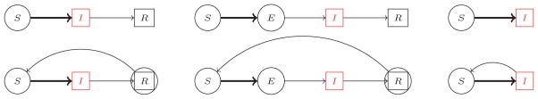
The models studied in this paper. Circles indicate the individuals who engage in mitigation behaviors. The red compartments indicate infectious individuals. Thick arrows indicate non-linear flow rates. Within the context of loss of immunity the recovered individuals may engage in some limited mitigation due to their inability to assess their own immunity.
Disease-risk mitigation is represented by either reducing contact volume, cx, or committing effort to avoiding contact with high-risk groups, altering PXY (t). We assume that mitigation is action intended to reduce the risk of infection so as to minimize the cost (disutility) of illness and illness avoidance. The only individuals engaged in mitigation are those who are either susceptible or unaware of their infectiousness/ immunity; we call these individuals “reactive”. In the models described in Figure 1 they comprise the S and E compartments (and to a lesser degree the R compartment in the presence of loss of immunity). Furthermore, we assume that all individuals within a particular compartment behave identically (we describe the behavior of a representative individual). Finally, we assume that all individuals are aware of their own symptomatically infectious status, and that these symptoms are readily recognizable by others.
1.2. Mixing Probability
The specification of the mixing probability presented here includes the classical incidence function as a special case. Effort committed to avoiding risk (either in terms of contact or affinity mitigation) is implicit in the estimated parameters (see Schmitz and Castillo-Chavez (1994) and Morin et al. (2010) for details). The mixing matrix, P = (Pij), composed of the mixing probabilities, satisfies three axioms at each moment t, (Blythe et al. (1991)):
0 ≤ Pij ≤ 1, for all i, j ∈ X,
ΣjPij = 1, for all i ∈ X,
cii(t)Pij = cjj(t)Pji, for all i, j ∈ X,
where X = {S, E, I, R}. Only a subset of states are attainable for a given compartmental model. The first two conditions imply that P is a matrix of conditional probabilities, and the third implies that activity incidence is symmetric. This symmetry induces an “activity-market” clearing condition. Each individual engages in a “normal” volume of activity for their disease state, ci, with individuals to mix with selected through the preferences/affinities expressed in Φ. It has been shown that the unique solution to these mixing axioms, and the solution that may describe all other mixing functions (at least asymptotically), is given by
| (2) |
where
and Φ = (ϕij) is a symmetric matrix (Blythe et al. (1991); Busenberg and Castillo-Chávez (1991); Castillo-Chavez et al. (1991)).
The affinity-based mixing preferences reflected in Φ represents the level of affinity mitigation effort as a function of the health status of individuals, the expected cost of illness and the cost of illness avoidance. This is the total cost of illness. Susceptible individuals seeking to minimize the expected cost of illness and the cost of illness avoidance can drive down the value of ϕSI = ϕIS directly. Recovered individuals seeking to maximize the benefits of R − S contacts can drive up ϕSR = ϕRS and lower herd immunity thresholds. Infectious individuals seeking to minimize the duration of the epidemic can drive down S−I and R−I contacts. This can further reduce ϕSI, ϕIR = ϕRI. In some cases, particular choices of Φ can induce a quarantine of infectious individuals (where PSI and PRI are very small, PIS and PIR are small, and PII is nearly 1).
We choose here a simple parameterization of Φ that ignores all strategies other than reduction of personal infection risk. Note that if all affinity values, ϕij, are equivalent, then the resulting mixing is based solely on availability, implying proportionate mixing. As already noted, we classify individuals in different health states as either reactive or nonreactive (either symptomatically infectious or recovered from such a state). Reactive individuals are assumed to avoid observably infectious individuals while nonreactive individuals mix equally with all health classes. That is, we exclude the possibility that individuals who are infected sequester themselves, or that individuals who are immune try to target specific individuals. We set the ϕij for all pairs of nonreactive states i and j to zero (there is no mitigation cost to be born if mixing is proportionate).
Under a contact mitigation strategy we assume that reactive individuals choose a contact volume, 0 ≤ cs = ce ≤ cr ≤ c. If there is no contact mitigation, all individuals make c contacts per unit time4. Under an affinity mitigation strategy, reactive individuals choose the effort they are willing to make to avoid infection, −vMax ≤ −v = ϕsi = ϕse ≤ ϕri ≤ 0 (the value vMax is the minimum, positive value that sets PSI equal to zero). A negative value for the affinity between a reactive class and a nonreactive class, e.g., ϕsi, reflects the desire of the reactive class to avoid the other (incentive or necessity is required for such contacts to occur), while a positive value reflects the desire to mix more than proportionately (a cost is willing to be born in order for the contact to occur; a behavior not considered here for reactive, non-reactive interactions). The cases where cr < c and/or ϕri < 0 occur only when the recovered individual is subject to a loss of immunity.
By way of example, consider a model where individuals are in states S, E, I, or R and where there is no loss of immunity. The affinity matrix will then take the form:
| (3) |
Note that S and E are both reactive since the latter do not know about their infection status, and I and R are both nonreactive.
1.2.1. The Heuristic for Equivalence
We consider two strategies for each of the model structures described in Figure 1. With the affinity mitigation strategy all individuals engage in the same amount of activity, c, but select/vary the people with whom they mix, PXY (t, Φ; c⃗). With the contact mitigation strategy reactive individuals (those who undertake disease-risk mitigation) are allowed to vary their contact volume, cx ≤ c, while having constant affinity, QXY (t, c⃗; Φ). The conditional probability PXY (t, Φ; c⃗) may thus take on different values over time as a function of both the availability of individuals within various states (X(t) and Y (t)) and their affinity for mixing (ϕxy); in contrast, QXY (t, c⃗; Φ) varies in time as a function of availability of individuals within various states and the volume of activity they are engaging in (all cx). We wish to show that within the affinity mitigation strategy there exists a choice of affinity, Φ, such that for any contact volume(s) chosen by the contact mitigation strategy, c⃗, the resulting dynamics of the two models are equivalent. To do this it is sufficient to equate the infection causing incidence between the two models:
| (4) |
First note that the left hand side, at time t, is a smooth function of Φ with maximum5 cI(t) and minimum 0. The right hand side is a smooth function of activity with the same maximum6 and minimum. It follows that for any given value of csQSI (t, c⃗; Φ) there exists a choice of affinity which equates the two.
It is also clear that by allowing both contact volume and affinity to vary (the “full” mitigative strategy) one does not introduce any further possible outcomes (the minimum is still zero and infectious contacts are not sought out, so the maximum holds at cI(t)). Therefore, addressing the pair directly results in an underdetermined system, and an unparsimonious characterization of behavior.
2. Results/ Examples
We now complete the steps involved in finding the change of variable, for a variety of epidemiological models, that equates contact mitigation with affinity mitigation. We begin with the SIR model and note that the basic structure of argument extends naturally to the SI and SEIR models both with and without reentry into the susceptible class. We do not equate the contact and affinity mitigation strategies directly. Rather, we equate the affinity mitigation strategy with the full model where both affinity and contact mitigations are allowed to take place (cs ≠ c and ν ≠ 0). We do this for 3 two reasons: 1) contact mitigation is a special case of the full model and 2) the resulting generality of the result leaves no doubt that the full mitigation strategy is indeed underdetermined. To translate the change-of-variable formula to be analogous to contact mitigation alone simply let ν = 0 and thus , the appropriate proportionate mixing ratio for the chosen contact volumes. The major result of our work may be summarized as follows
Theorem 1 (Model Equivalence)
If new infection only occurs in a reactive susceptible class (S) due to contact with a non-reactive infectious class (I) (one that is aware of its infection status) any change in incidence created both by allowing both contact and affinity mitigation can be achieved by either mitigative strategy alone.
Epi-Corollary 1
For standard SIR, SEIR, and SI models with and without loss of immunity, all possible solutions generated by varying the volume of contacts can be generated by a choosing with whom to mix. Furthermore, combining the two effects offers no additional outcomes. We conclude that in terms of their impact on epidemics, there is at least formal equivalence between contact and affinity mitigation strategies.
The Theorem and resulting Epi-Corollary (the outcomes of which are demonstrated in the following subsections) point out important questions when it comes to fashioning epidemic models with individual-based mitigative strategies. From a phenomenological sense, it suffices to allow for only a single strategy (contact or affinity mitigation) so long as there are no limitations on choice, and if a mixture of strategies is allowed within the population then there will be identifiability issues with respect to parameter estimation from data that does not explicitly detail the behavioral effects the population undertakes.
2.1. SIR full calculation
We assume that the only mitigation response is by the susceptible class, and define c to be the contact rate – the per unit time volume of contacts – for all non-reactive classes7 and assert that cs ≤ c. The calculations follow.
For the affinity mitigation strategy, let PSI be the probability structure as defined above:
| (5) |
with , MR = 1, and . Also define for the full mitigation strategy
| (6) |
with , NR = 1, and . Assume that cs and ν are chosen; thus we are tasked with finding a value for v such that for a given state of the world (S(t), I(t), and R(t)) we have
| (7) |
Leaving QSI intact and solving for v results in
| (8) |
We first show that it will never be the case that . Thus neither root, v±, is complex or negative, and v may then be chosen from its valid range to make the affinity mitigation strategy equivalent to the full mitigation strategy.
We show that by decomposing QSI in order to solve for ν:
| (9) |
If it is true that then the inequality (9) is always satisfied with positive ν (i.e., both roots are either complex or negative and thus for the positive ν axis the quadratic is positive). By assuming that cs ≤ c we may show this (noting that ):
Therefore we have that v+, the positive root of equation (8), is a candidate substitution for equality between the two strategies so long as . The upper bound is constructed by solving for when PSI = 0; beyond this point PSI < 0. The validity of v+ can be shown directly by noting
| (10) |
and then building each side up to
2.2. Loss of Immunity: SIRS
The problem posed by the SIRS model is that recovered individuals cannot assess whether or not they’ve lost immunity. For single outbreak epidemics where the loss of immunity is on a much longer time scale than the epidemic spread, we should be able to omit the dynamic. In general, however, loss of immunity imposes some uncertainty for the recovered individual. Let k ∈ [0, 1] be a function of time since the individual has recovered from infection, the state of the world, or any other such metric. Regardless of the form of the loss of immunity function the affinity matrix will have the form
| (11) |
or
| (12) |
Furthermore, in the full mitigation strategy we assume that recovered individuals may choose to adjust their contact volumes such that 0 ≤ cs ≤ cr ≤ c. Thus equating incidence rates between the two strategies implies that
| (13) |
where . The quantities k and κ play no role in the equivalence other than through the requirement that k, κ ≤ 1.
If we denote the avoidance of infectious individuals by immune individuals via u < v and μ < ν the proof is less straightforward. However, one may then return to the parameterization of u = kv (μ = kν) because we left the exact nature of k and κ general enough to account for any possible form of u and μ.
2.3. Unknown Infection: SEIR/ SEIRS
Consider the impact of latent infection, and equate only the susceptible-infectious (infection causing) incidence between the strategies (even though latent individuals engage in mitigative behavior). Since we are seeking a change of variables that equates infection causing incidence, and thus the trajectory of the state variables, this suffices. The calculations are fundamentally identical to the SIR case with
| (14) |
and . Following the exact same arguments as in the SIRS case results in
| (15) |
with , as the change of variable formula for the SEIRS model.
2.4. No Recovery: SI/SIS
A single calculation holds for both the SI and SIS models. Note that since S + I = 1 we have . Equating the incidences results in
| (16) |
2.5. The Problem of Asymptomatic Individuals
What effects do the decisions of asymptomatic individuals have on mixing probabilities? Recall that these are conditional probabilities, i.e., ΣY PXY = 1, and if v is some avoidance effort we have that (PSI decreases with increased affinity mitigation effort) and (PSA increases with affinity mitigation effort). The fact that PSI decreases with avoidance is clear. Since asymptomatic individuals do not know of their infectiousness, they seek to avoid infectious individuals and thus distribute their remaining activity evenly about the remaining indistinguishable states, resulting in an increase in their mixing with susceptible individuals. However, under contact mitigation, reactive individuals may choose to participate in no activity, cs = ca = 0, and thus total incidence is 0. It follows that affinity and contact mitigation strategies are not, in general, equivalent in the presence of asymptomatic infection! If infectious individuals engage in risk-avoidance behavior, mitigation creates additional infection as in Meloni et al. (2011). In general, because contact mitigation always results in a decrease in incidence, we may assert that only when affinity mitigation does not result in more infections than proportionate mixing may it be possible to equate both the contact and affinity mitigation strategies. Thus it becomes a study of the sign of : when positive, an increase in affinity mitigation increases the infection risk, and when negative, an increase in affinity mitigation decreases the infection risk. This expression is quite complicated and the conditions for which it is negative are complex. However, as a first step to understanding this we may consider the end points: an absence of affinity mitigation (v = 0) and the maximum affinity mitigation response (v = vMax → PSI = 0).
As an illustration, consider the simplest model where loss of infection implies immediate and permanent immunity and asymptomatic infection is simply a stage before symptomatic infection. When there is no affinity mitigation, the incidence for the affinity model is given by Inc0 := c (βI I + βAA). At vMax avoidance has driven PSI to 0 and thus the incidence, which is unobservable at that moment, is strictly between susceptible and asymptomatically infectious individuals given by IncM := cβAP̂SA. In general the incidence is of course Inc := c (βI PSI + βAPSA).
Consider first solving for Inc0 = IncM. This results in a quadratic in v (technically vMax) with roots v±. From the sign of the coefficients we may assert that for when vMax ∈ (v−, v+) (implying that v± ∈ ℝ) then IncM >Inc0, or more simply that the effective quarantine (produced by individual affinity mitigation actions) of symptomatically infectious individuals results in more new infection than “doing nothing”. In the case that v± ∈
 then all values8 of vMax produce fewer infections than proportionate mixing. The general conditions for IncM > Inc0 favor processes that produce (or contain in some a priori sense) a great deal of asymptomatic individuals:
| (17) |
The bound on I(t) is a surface on which the third requirement gives that βA = βI. The bounding surface for I(t) (the second condition) compromises only 1.2% of the volume of the total state-space, the unit tetrahedron in (S, A, I). Couple that with the fact that the third condition comprises 58.2% of the valid range of . The conditions in which selective mixing results in more infection than proportionate mixing are extremely restrictive: requiring widespread asymptomatic infection, almost no symptomatic infection, and roughly equivalent infectiousness in both cases, .
If asymptomatic individuals do not subsequently become symptomatic, i.e. the two path diagram in Figure 2, affinity mitigation will never generate more infection than proportionate mixing. In the two-path asymptomatic model a subset of the recovered/immune population engages in mitigation as if they were susceptible (RA(t)). Thus, the S – A contacts may become diluted enough such that vMax > v+ will always be true. With the two-path model we may even extend this result to say that if
Figure 2.

Two examples of models with asymptomatic infections. On the left, asymptomatic infection is a stage before symptomatic infection. To the right there are two separate infection paths: individuals either become symptomatically or asymptomatically infectious and eventually recover from this state. When asymptomatic, or after recovering from asymptomatic infection in the two-path model, individuals continue to engage in mitigation because they are unaware of their infectious status.
| (18) |
where , then any level of affinity mitigation is better than doing nothing, and thus equivalence between the mitigation strategies may be possible.
3. Discussion
It has been shown that describes all mixing functions that meet the mixing conditions of Busenberg and Castillo-Chávez (1991). While specific discussion of the mechanism by which individuals make contact is omitted here (see Hadeler (2012) for more detail) we assume that individuals make contacts based on their preferences, the availability of others, and the preferences of others. is the availability of I type individuals, who are then paired with others as a function of the jointly determined affinity for that pairing to occur. Quantities such as MS = 1 −Σx ϕXSX(t) are a measure of the unmet desires of other groups to mix with S type individuals. Thus is a normalized measure of the contacts to be made with infectious individuals that are “left-over” after contacts made in the purely desirous sense (e.g., PI (t)ϕSI) are made. This is further scaled by MS to measure the left-over contacts that need be met for the susceptible group.
By contrast, affinity-based mixing found in population genetics and behavioral ecology literature of Karlin, Levin and Segel, and others (see Karlin and McGregor (1972); Levin and Segel (1982)), and in the context of epidemiology via works such as by Koopman et al. (1989) and Hyman and Li (1997), allows individuals to encounter others at random and then decide to mate or pair per the probability α(i, j). In these two-sex formulations it is standard that one mate (first argument) does the selecting. Therefore, the proportion of all pairs probability of an S pairing with an I as
| (19) |
where αij are all non-negative affinities between groups (not symmetric). It should be clear that this form does not meet the third mixing condition (that all contacts made by group i with group j are equivalent to the contacts group j makes with group i) because of the asymmetry between intergroup preferences (αij ≠ αji). The mechanism described by such a formulation also assumes a process driven by only desire and availability. In other words there is no activity-market clearing mechanism as in PSI (t) (i.e., not all individuals need make a requisite volume of contacts). Individuals within this frame work will not settle for left-over contacts and may engage in fewer contacts than they are allowed to maximally make. However, from the individual perspective within the context of epidemics, this can be translated to the full mitigation strategy (which we’ve described as underdetermined). This is more or less what was done in Hyman and Li (1997) with proportionate availabiliy, and can be made equivalent to the affinity mitigation strategy as shown above.
While finding conditions where equivalence may hold for models that include asymptomatically infectious individuals is tedious, we have encountered numerical examples where this is true. These occur where affinity mitigation is less costly than contact mitigation (a situation perhaps most true for the working poor). In this case the likelihood of a choice causing cs = 0 is low. Thus with cs bounded away from zero the equivalence arguments for the one-path SAIR model reduces to those in the SEIR model. We also found that conditions where undertaking affinity mitigation in the presence of asymptomatic individuals will rarely result in a worse scenario than doing nothing.
Note, though, that the cost of each strategy need not be the same. Infectious disease imposes two costs on individuals: the cost of disease, CD, and the cost of mitigation, CM. In both cases (contact or affinity mitigation) the cost of disease comprises the disutility of illness (pain and suffering), the cost of treatment, and forgone earnings caused by disability or hospitalization. The cost of mitigation, however, depends on the strategy applied. With the contact mitigation strategy the cost of mitigation comprises any forgone earnings due to the reduction in contact volume, i.e. CM ≡ contact value= cS. With the affinity mitigation strategy the cost of mitigation is the cost of avoiding infectious individuals, i.e. C̃M ≡ affinity=v.
To evaluate the implications of differences in the cost of contact and affinity mitigation we assume that people aim to minimize the cost of containing infection risk to an acceptable level. Moreover, they do this by choosing between these two mitigation strategies. That is, they identify which combination of strategies is most cost-effective. If we describe the cost of disease as a function of the incidence associated with each of two strategies, C(cPSI (t, Φ; c⃗), csQSI (t, c⃗; Φ)), then a first order necessary condition for this to be minimized is that the marginal value of the reduction in the cost of disease under each strategy is equalized. This requires that . It follows that if the marginal cost of affinity mitigation is less than the marginal cost of contact mitigation, and the individual will commit effort to selective mixing rather than sequestration. is identical to asserting that
for all positive v. Consider the equivalent problem of −P4 > 0. The Routh-Hurwitz conditions then state that if −A > 0, BC > AD, and BCD < AD2+B2E then all roots of −P4 are in the left-hand plane (i.e., with negative real part). Therefore, ∀ v > 0 we have implying that affinity mitigation will be preferred to contact mitigation wherever people prefer to avoid infectious individuals (v > 0).
In Figures 3 – 5 we show the region of S–I space where the Routh-Hurwitz criterion is met if people are minimizing the cost of containing disease risk within acceptable limits. Overall, as c increases, the individual has more contact-capital with which to work with and thus is more inclined to sacrifice a portion of those contacts. For c ≤ 1 there is insufficient contact-capital and over the entire phase-space affinity mitigation is preferred to contact mitigation. For 1 < c < 4.6, in our numerical example, the results are mostly intuitive; it is more costly to meet an infectious risk target by choosing with whom to mix than by choosing how much to mix as long as infectious individuals are a large proportion of the population. However, for low levels of infection, it is more cost effective to use affinity mitigation. This partly reflects the fact that we have considered only the case where all the roots of P4 are in the left hand plane. Other configurations for the roots of P4 could yield different results.
Figure 3.

For contact volume less than 4.6 the resuls are largely intuitive. When the infectious population out numbers the susceptible population a relative small sized recovered population induces contact mitigation to be favored (shown for small S(t) and moderate I(t)). Less intuitively, and possibly due to the fact that we’ve analyzed only one possible condition for the polynomial P4, is when S(t) dominates the population and still there are cases where contact mitigation is favored (e.g., when S(t) + I(t) ≈ 1).
Figure 5.

Shown here are 3 values for c > 4.6 which demonstrate the general trend for the shape of the shaded region (where affinity mitigation is favored). For c > 50 the shaded region partitions the phase space into three regions by separating the region where contact mitigation is favored.
Note that for c ≥ 4.6 the shaded region “doubles back” into the permissable phase-space and presents a set of counterintuitive nonlinearities. Thus, for c ≥ 4.6 we may have the case for a given S(t) there exists 0 < I1 < I2 < I3 < 1 such that for I(t) ∈ [0, I1] ∪ [I2, I3] affinity mitigation is preferred, but for I(t) ∈ (I1, I2) ∪ (I3, 1] contact mitigation is preferred. The middle region of (I1, I2) is not intuitive because it contains more recovered/immune individuals than in (I2, I3) and thus more opportunities for infection-free contacts. This may again be attributed to our method. Figure 6 has the results for c [0, 50] distilled to a single metric: the proportion of the phase space for which our method says that affinity mitigation is preferred to contact mitigation. What these figures measure is the likelihood that affinity mitigation will dominate contact mitigation given the total number of contacts that could be made. Since the cost of avoiding a single contact is being held constant, an increase in the number of available contacts is equivalent to an increase in the relative cost of affinity mitigation. So the figures measure the sensitivity of choice of affinity mitigation over contact mitigation to the cost of mixing.
Figure 6.

Shown here are the nominal contact volumes required for affinity mitigation to be preferred over contact mitigation for particular proportions of the phase space (the horizontal axis).
Which strategy, contact or affinity mitigation, is selected depends on the relative cost of each strategy. Yet most studies of the effect of human behavior on epidemiology assumes that the contact mitigation strategy operates. This is partly because the contact volume is easier to understand and to estimate using data (although there are problems with this if the data do not reflect effects such as monogamy9). Indeed, determining whether people are engaging in fewer contacts or an altering of contact type is hard (see Khan et al. (2013) for a detail on airline behavior given the 2009 A(H1N1) epidemic). The choice of mitigation strategy does matter, however. We have shown that while the two strategies may have the same epidemiological consequences, the cost of illness to the individual and the cost of an epidemic to society will potentially be different. Where people are able to select between contact and affinity mitigation, though, they will make choices that minimize the cost of illness to themselves and the cost of an epidemic to society.
Figure 4.

The “doubling back” of the region where selective mixing is favored is shown here for c = 4.6 and 5.6. The pattern of the “upper edge” decreasing and the cusp reaching further into the S – I plane persists as c increases. The region where affinity mitigation is favored rapidly shifts at first (when small gains in c represent large proportionate changes in contact-capital) and then slows as c becomes quite large.
Footnotes
This publication was made possible by grant number 1R01GM100471-01 from the National Institute of General Medical Sciences (NIGMS) at the National Institutes of Health. Its contents are solely the responsibility of the authors and do not necessarily represent the official views of NIGMS.
This simplification is strictly for the purpose of computations and does not alter the results so long as symptomatically infectious individuals do not engage in greater than normal levels of activity.
If PSI (t) exceeded the availability of infectious individuals there would exist some incentive to get sick.
The conditional probability QSI (t) is also assumed to have a maximum of I(t) since it should not exceed the availability of infectious individuals without some incentive to seek them out.
This implies that each non-reactive group has the same contact volume between the two models PSI and QSI. We take this case, where ci = cr =: c, simply to save some notation.
The affinity value which drives PSI (t) to 0 is a function of the state variables.
This is a long standing problem. See Oster (2005) for a treatment of low and high risk groups and Morris (2010) for a commentary on the various problems/inconsistencies in trying to tease this effect out of data.
Publisher's Disclaimer: This is a PDF file of an unedited manuscript that has been accepted for publication. As a service to our customers we are providing this early version of the manuscript. The manuscript will undergo copyediting, typesetting, and review of the resulting proof before it is published in its final citable form. Please note that during the production process errors may be discovered which could affect the content, and all legal disclaimers that apply to the journal pertain.
References
- Arino J, Jordan R, Van den Driessche P. Quarantine in a multi-species epidemic model with spatial dynamics. Mathematical biosciences. 2007;206 (1):46–60. doi: 10.1016/j.mbs.2005.09.002. [DOI] [PubMed] [Google Scholar]
- Blythe S, Castillo-Chavez C, Palmer M. Toward a unified theory of sexual mixing and pair formation. Mathematical Biosciences. 1991;107 (2):379–405. doi: 10.1016/0025-5564(91)90015-b. [DOI] [PubMed] [Google Scholar]
- Busenberg S, Castillo-Chávez C. A general solution of the problem of mixing of subpopulations and its application to risk-and age-structured epidemic models for the spread of AIDS. Mathematical Medicine and Biology. 1991;8 (1):1. doi: 10.1093/imammb/8.1.1. [DOI] [PubMed] [Google Scholar]
- Castillo-Chavez C, Busenberg S, Gerow K. Pair formation in structured populations. Differential Equations with Applications in Biology, Physics and Engineering. 1991:47–65. [Google Scholar]
- Castillo-Chavez C, Castillo-Garsow CW, Yakubu AA. Mathematical models of isolation and quarantine. JAMA: The Journal of the American Medical Association. 2003;290 (21):2876–2877. doi: 10.1001/jama.290.21.2876. [DOI] [PubMed] [Google Scholar]
- Chan M, Bradley M, Bundy D. Transmission patterns and the epidemiology of hookworm infection. International journal of epidemiology. 1997;26 (6):1392–1400. doi: 10.1093/ije/26.6.1392. [DOI] [PubMed] [Google Scholar]
- Chowell G, Viboud C, Wang X, Bertozzi SM, Miller MA. Adaptive vaccination strategies to mitigate pandemic influenza: Mexico as a case study. PLoS One. 2009;4 (12):e8164. doi: 10.1371/journal.pone.0008164. [DOI] [PMC free article] [PubMed] [Google Scholar]
- Fenichel EP, Castillo-Chavez C, Ceddia M, Chowell G, Parra PAG, Hickling GJ, Holloway G, Horan R, Morin B, Perrings C, et al. Adaptive human behavior in epidemiological models. Proceedings of the National Academy of Sciences. 2011;108 (15):6306–6311. doi: 10.1073/pnas.1011250108. [DOI] [PMC free article] [PubMed] [Google Scholar]
- Fenichel EP, Wang X. Modeling the Interplay Between Human Behavior and the Spread of Infectious Diseases. Springer; 2013. The mechanism and phenomena of adaptive human behavior during an epidemic and the role of information; pp. 153–168. [Google Scholar]
- Gregson S, Gonese E, Hallett TB, Taruberekera N, Hargrove JW, Lopman B, Corbett EL, Dorrington R, Dube S, Dehne K, et al. Hiv decline in zimbabwe due to reductions in risky sex? evidence from a comprehensive epidemiological review. International Journal of Epidemiology. 2010;39 (5):1311–1323. doi: 10.1093/ije/dyq055. [DOI] [PMC free article] [PubMed] [Google Scholar]
- Gross T, DLima CJD, Blasius B. Epidemic dynamics on an adaptive network. Physical review letters. 2006;96 (20):208701. doi: 10.1103/PhysRevLett.96.208701. [DOI] [PubMed] [Google Scholar]
- Hadeler K. Pair formation. Journal of mathematical biology. 2012;64 (4):613–645. doi: 10.1007/s00285-011-0454-0. [DOI] [PubMed] [Google Scholar]
- Herrera-Valdez M, Cruz-Aponte M, Castillo-Chavez C. Multiple outbreaks for the same pandemic: Local transportation and social distancing explain the different” waves” of a-h1n1pdm cases observed in méxico during 2009. Mathematical Biosciences and Engineering (MBE) 2011;8 (1):21–48. doi: 10.3934/mbe.2011.8.21. [DOI] [PubMed] [Google Scholar]
- Hethcote HW. The mathematics of infectious diseases. SIAM review. 2000;42 (4):599–653. [Google Scholar]
- Hyman JM, Li J. Behavior changes in sis std models with selective mixing. SIAM Journal on Applied Mathematics. 1997;57 (4):1082–1094. [Google Scholar]
- Karlin S, McGregor J. Polymorphisms for genetic and ecological systems with weak coupling. Theoretical population biology. 1972;3 (2):210–238. doi: 10.1016/0040-5809(72)90027-5. [DOI] [PubMed] [Google Scholar]
- Khan K, Eckhardt R, Brownstein JS, Naqvi R, Hu W, Kossowsky D, Scales D, Arino J, MacDonald M, Wang J, et al. Entry and exit screening of airline travellers during the a (h1n1) 2009 pandemic: a retrospective evaluation. Bulletin of the World Health Organization. 2013;91 (5):368–376. doi: 10.2471/BLT.12.114777. [DOI] [PMC free article] [PubMed] [Google Scholar]
- Koopman JS, Simon CP, Jacquez JA, Park TS. Mathematical and statistical approaches to AIDS epidemiology. Springer; 1989. Selective contact within structured mixing with an application to hiv transmission risk from oral and anal sex; pp. 316–348. [Google Scholar]
- Leach M, Scoones I, Stirling A. Governing epidemics in an age of complexity: Narratives, politics and pathways to sustainability. Global Environmental Change. 2010;20 (3):369–377. [Google Scholar]
- Levin SA, Segel LA. Models of the influence of predation on aspect diversity in prey populations. Journal of mathematical biology. 1982;14 (3):253–284. doi: 10.1007/BF00275393. [DOI] [PubMed] [Google Scholar]
- Mah TL, Halperin DT. Concurrent sexual partnerships and the hiv epidemics in africa: evidence to move forward. AIDS and Behavior. 2010;14 (1):11–16. doi: 10.1007/s10461-008-9433-x. [DOI] [PubMed] [Google Scholar]
- Meloni S, Perra N, Arenas A, Gómez S, Moreno Y, Vespignani A. Modeling human mobility responses to the large-scale spreading of infectious diseases. Scientific reports. 2011:1. doi: 10.1038/srep00062. [DOI] [PMC free article] [PubMed] [Google Scholar]
- Mercer CH, Copas AJ, Sonnenberg P, Johnson AM, McManus S, Erens B, Cassell JA. Who has sex with whom? characteristics of heterosexual partnerships reported in a national probability survey and implications for sti risk. International Journal of Epidemiology. 2009;38 (1):206–214. doi: 10.1093/ije/dyn216. [DOI] [PubMed] [Google Scholar]
- Merl D, Johnson LR, Gramacy RB, Mangel M. A statistical framework for the adaptive management of epidemiological interventions. PloS One. 2009;4 (6):e5807. doi: 10.1371/journal.pone.0005807. [DOI] [PMC free article] [PubMed] [Google Scholar]
- Morin BR, Castillo-Chavez C, Hsu Schmitz SF, Mubayi A, Wang X. Notes from the heterogeneous: a few observations on the implications and necessity of affinity. Journal of Biological Dynamics. 2010;4 (5):456–477. doi: 10.1080/17513758.2010.510212. [DOI] [PubMed] [Google Scholar]
- Morin BR, Fenichel EP, Castillo-Chavez C. Sir dynamics with economically driven contact rates. Natural Resource Modeling. 2013 Nov;26 (4):505–525. doi: 10.1111/nrm.12011. [DOI] [PMC free article] [PubMed] [Google Scholar]
- Morris M. Concurrent partnerships and syphilis persistence: new thoughts on an old puzzle. Sexually transmitted diseases. 2001;28 (9):504–507. doi: 10.1097/00007435-200109000-00005. [DOI] [PubMed] [Google Scholar]
- Morris M. Barking up the wrong evidence tree. comment on lurie & rosenthal, concurrent partnerships as a driver of the hiv epidemic in sub-saharan africa? the evidence is limited. AIDS and Behavior. 2010;14 (1):31–33. doi: 10.1007/s10461-009-9639-6. [DOI] [PMC free article] [PubMed] [Google Scholar]
- Oster E. Sexually transmitted infections, sexual behavior, and the hiv/aids epidemic. The Quarterly Journal of Economics. 2005;120 (2):467–515. [Google Scholar]
- Plowright RK, Sokolow SH, Gorman ME, Daszak P, Foley JE. Causal inference in disease ecology: investigating ecological drivers of disease emergence. Frontiers in Ecology and the Environment. 2008;6 (8):420–429. [Google Scholar]
- Schmitz S-FH, Castillo-Chavez C. Modeling the AIDS Epidemic: Planning Policy and Prediction. New York: Raven Press Limited; 1994. Parameter estimation in non-closed social networks related to dynamics of sexually transmitted diseases. [Google Scholar]