Abstract
Recently we have proposed the use of Tikhonov regularization with temporal smoothness constraints to estimate the BOLD fMRI hemodynamic response function (HRF). The temporal smoothness constraint was imposed on the estimates by using second derivative information while the regularization parameter was selected based on the generalized cross-validation function (GCV). Using one-dimensional simulations, we previously found this method to produce reliable estimates of the HRF time course, especially its time to peak (TTP), being at the same time fast and robust to over-sampling in the HRF estimation. Here, we extend the method to include simultaneous temporal and spatial smoothness constraints. This method does not need Gaussian smoothing as a pre-processing step as usually done in fMRI data analysis. We carried out two-dimensional simulations to compare the two methods: Tikhonov regularization with temporal (Tik-GCV-T) and spatio-temporal (Tik-GCV-ST) smoothness constraints on the estimated HRF. We focus our attention on quantifying the influence of the Gaussian data smoothing and the presence of edges on the performance of these techniques. Our results suggest that the spatial smoothing introduced by regularization is less severe than that produced by Gaussian smoothing. This allows more accurate estimates of the response amplitudes while producing similar estimates of the TTP. We illustrate these ideas using real data.
Keywords: ER-fMRI, HRF estimation, Tikhonov regularization, GCV
Introduction
Blood oxygen level dependent (BOLD) signal in fMRI (Ogawa et al 1990) has become one of the main imaging tools to study the brain in vivo. Common assumptions made in fMRI data analysis are the linearity and time invariance of the observed time series (Friston et al 1994). While in general these assumptions are not true (Boynton et al 1996, Friston et al 2000), they produce reasonable approximations in many practical situations. A linear and time-invariant system can be characterized by an impulse response function that when convolved with the system’s input, defines its output. For BOLD fMRI signals, the input of the system is a given stimulation pattern while the output is the observed time series that is compounded by noise due to the scanning process and biological processes. The so-called hemodynamic response function (HRF) plays the role of the impulse response function at each voxel of the brain.
The detection of functional activity in fMRI is often carried out by assuming some fixed shape of the HRF and solving a voxel-wise regression model (Friston et al 1995). Though this approach has rendered great services to the neuroimaging community, it has the intrinsic problem of biasing detection toward the assumed shape. This opens the possibility of a loss of statistical power in situations where the elicited HRF greatly differs from the assumed shape, as previously reported in epileptic (Lu et al 2006) and stroke (Bonakdarpour et al 2007) patients as well as in normal subjects (Fuhrmann Alpert et al 2007, Marrelec et al 2003). It has been proposed that the estimated HRF time course can be used to extract valuable information about the timing of neuronal events in different regions of the brain (Menon et al 1998, Miezin et al 2000). While caution should be exercised in this type of analysis due to differences in vasculature across brain regions (Miezin et al 2000), this is potentially another useful application of fMRI. Thus, estimating HRF without assuming any shape is very desirable even though it is a complex problem confounded by different factors including low signal-to-noise ratios and nonlinearities of the BOLD fMRI signals. In addition, the huge number of voxels that characterizes the fMRI images makes this problem computationally challenging. Different approaches have been proposed to estimate the HRF time course. These include window averaging (Dale and Buckner 1997), FIR (Dale 1999, Lange et al 1999), Bayesian regularization (Goutte et al 2000, Marrelec et al 2003, Woolrich et al 2004) and different versions of Tikhonov regularization (Vakorin et al 2007, Zhang et al 2007). Recently, we proposed (Casanova et al 2008) the use of Tikhonov regularization with boundary and temporal smoothness constraints (Goutte et al 2000, Marrelec et al 2003) for HRF estimation. We explored its properties in different contexts using one-dimensional simulations, and we found it to be fast and reliable for estimating HRF. The regularization parameter was selected using generalized cross-validation (Carew et al 2003, Wahba 1990). Here, we extend the algorithm by adding a spatial smoothness constraint. The basic idea is to use information from neighboring voxels when estimating the HRF at a given voxel. The spatial smoothness constraint is imposed by using second derivative information. Similar ideas have been implemented before in the context of the MEG-EEG inverse problem by Pascual-Marqui (1994). Penny et al (2005) used spatial priors based on second derivative information similar to those used by LORETA in their Bayesian approach for fMRI data analysis. We relied on Tikhonov regularization with GCV to choose the regularization parameter. Our method imposes not only spatial but also temporal smoothness on the estimated HRF and does not require prior Gaussian smoothing of the images which is often performed in fMRI data analysis as a preprocessing step. Though useful in many respects, the smoothing step introduces distortions in the data. These distortions are particularly evident in voxels at the edges of the brain since voxels belonging to the background are used in the smoothing operation introducing a bias toward zero of the signal. Here we present the results of different two-dimensional simulations comparing the relative performance of these two different versions (temporal versus spatio-temporal) of Tikhonov regularization. We focus these simulations on examining the impact of the smoothing introduced by the Gaussian filter or by the spatio-temporal Tikhonov regularization when estimating the HRF. Special attention is directed to the edges of the brain and activations. We also use real data to illustrate these concepts.
Materials and methods
Linear model
If we assume that the fMRI response is linear and time invariant, then the BOLD signal y at a given voxel can be represented as
| (1) |
where y is a N × 1 vector representing the fMRI signal from a voxel, N is the number of time samples, X = [X1X2 … XNe], h = [h1, h2 … hNe]T, where Xi and hi are the stimulus convolution matrix and the vector representation of the HRF corresponding to the event i, respectively and Ne is the number of events. The stimulus convolution matrix Xi is generated based on the stimulus sequence. The dimension Ns of the vector hi determines a fixed time-span of the HRF and its time resolution. Finally, n is additive noise with covariance matrix V.
In this work, we model the drift usually observed in the fMRI times series using orthogonal polynomials, the number of events was set to Ne = 1, and the noise was considered to be independent and identical distributed (i.i.d.) Gaussian (V = I). In order to account for the autocorrelation present in the fMRI time series, the temporal covariance structure should be estimated based on the acquired data (Bullmore et al 2001, Worsley et al 2002) and used to pre-whiten the fMRI time series before applying the model. So, our linear model will be defined as
| (2) |
where P is a N × M matrix containing a basis of M orthonormal polynomial functions that takes a potential drift into account. The highest order of the polynomials is M − 1 and l is the M × 1 vector of the drift coefficients. We took M = 3 in our implementation to model first- and second-order drift commonly observed in fMRI times series.
HRF estimation methods based on regularization
Tikhonov regularization with temporal smoothness constraint (Tik-GCV-T)
The Tikhonov solution of (2) with temporal smoothness constraining (Casanova et al 2008) is obtained by solving the following optimization problem:
| (3) |
where λ is the regularization parameter. The solution of (3) is given by
| (4) |
The last equality results from orthogonality of P in our case. The resulting X⊥ amounts to removing the drift from the stimulus convolution matrix (Liu et al 2001). L1 is a (Ns − 2)(Ns − 2) matrix embodying the discrete second derivative (Marrelec et al 2003) and we assumed the boundary conditions h1 = hNs = 0 (Goutte et al 2000) that implies removing two columns from matrix X. For the particular case when λ = 0 this method reduces to the common least squares (LS).
Tikhonov regularization with spatio-temporal smoothness constraints (Tik-GCV-ST)
We have implemented a version of Tikhonov regularization with both spatial and temporal smoothness regularization. The basic idea is to estimate the HRF at a given voxel and its neighbors simultaneously using an additional second derivative spatial smoothness constraint. The same temporal smoothness and boundary constraints used in equation (3) are imposed on all HRFs being simultaneously estimated. The Tikhonov functional for a given voxel is then defined by
| (5) |
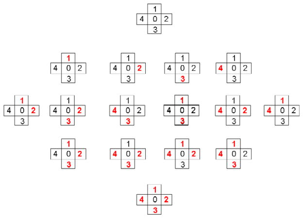
where Nn is the number of cardinal neighboring voxels (see figure 1) based on a four neighborhood system, h̃ is the (Ns − 2) * (Nn + 1) × 1 vector that contains the stacked HRFs of the voxel of interest and its Nn neighbors. Similarly ỹ and l̃ are the N(Nn + 1) × 1 and M(Nn + 1) × 1 vectors containing the stacked data and drift parameters. The symbol ⊗ is the matrix kronecker product. L1 is the same as in equation (3) and L2 (2D Laplacian) and are (Ns − 2) × ((Ns − 2)(Nn + 1)) matrices that embody spatial second derivative constraints on the voxel of interest and its neighbors. The two-dimensional discrete Laplacian L2 is computed by assigning to the diagonal elements the number of neighbors of the analyzed voxel. It has to be noted that this is not used by LORETA (Pascual-Marqui et al 1994) nor the one used in Penny et al (2005) since the weight we assigned to the voxel of interest is Nn. Our Laplacian by itself is singular but our choice for renders the matrix Ls non-singular. Specifically, we chose it as the second derivative with weight fixed to −2 for a given neighboring voxel and 1 for the voxel of interest. The advantage of our choice of the second derivative constraint is that it avoids the bias toward zero of parameter estimates in the voxels at the boundary of the brain produced by Gaussian smoothing of the data or other choices of regularization operators. The Ls, h̃, l̃, ỹ displayed after equation (5) correspond to the situation when the voxel has all of its four neighbors present (see figure 1) or it does not lie in the brain boundary. The computation of Ls, Lt requires for each voxel a customized treatment according to the number of neighboring voxels Nn.
Figure 1.
All possible situations for the 4-neighborhood system are shown. The first row corresponds to the case when the voxel is not in the boundary of the brain (Nn = 4). The second, third, forth and fifth correspond to the cases when 1, 2, 3 or 4 voxels are missing or Nn = 3, 2, 1, 0, respectively. The missing ones are highlighted in red bold.
The ĥ that minimizes the problem defined in equation (5) is
| (6) |
where
After simultaneously estimating the HRFs for the voxel of interest and its neighbors, we retain ĥ0 as the final estimator of the HRF and discard the others.
The selection of the regularization parameter in both algorithms is based on generalized cross-validation GCV (Golub et al 1979, Wahba 1990). In our implementation, we used a MATLAB package for regularization available publicly at http://www2.imm.dtu.dk/~pch/Regutools/regutools.html) (Hansen 1994).
Simulated data
Signal generation
We generate sequences of two-dimensional 17 × 17 images, where activations have been added in different positions, to simulate one slice of the fMRI time series. For the voxels inside the activated regions, single event sequences generated with a geometric probabilistic distribution of the intertrial intervals (ITI) (Burock et al 1998) were convolved with the difference of gamma densities function (Worsley et al 2002)
where a1 = 6, a2 = 12, b1 = b2 = 0.9, c = 0.35, HR = 0.3. In this case the time to peak (TTP) was 5.4 s, the hemodynamic response (amplitude) HR was the same for all activated voxels.
The fMRI signal was simulated by putting together the sequence of events at a finer temporal grid. The event onsets were approximated to the nearest point in the grid and then convolved with the test function h(t). The resulting signal was under-sampled to TR = 1 s and Gaussian white noise with a fixed standard deviation was added to the data together with a quadratic drift. The durations of the experiment and the HRF were set to 310 s and 20 s, respectively.
Measures of performance
The comparative results presented below are based on the relative errors for TTP, HR and the root mean square error (RMS) given in percentages. We estimate TTP and HR as
where dt is the time resolution of the HRF estimation. The measures of performance we will use in our simulations are
| (7) |
| (8) |
| (9) |
where Nr, Nav stand for the number of realizations of the noise and the number of activated voxels, respectively. and are the true and estimated amplitudes of the response for individual voxels inside the simulated activation. and TTPtrue are the estimated and true time to peak for individual voxels inside the simulated activation. The latter is constant for all activated voxels (5.4 s). Finally, and stand for the estimated and true HRF samples for individual voxels inside the simulated activation. These measures of the relative error were computed for the most efficient design (Dale 1999) generated using a random walk of 1000 iterations (Casanova et al 2008). The efficiency when optimizing the designs was computed according to Dale (1999) and taking into account the drift (Liu et al 2001).
Simulations
In all simulations we assumed that the HRF is smooth and that the fMRI signal was linear and time invariant, common assumptions in fMRI data analysis. The amplitude of the HRFs was the same for all activated voxels (HR = 0.3) in all simulations with the exception of the simulation 1 c) where a spatially varying profile of the HRF amplitudes was simulated. We compare the performance of Tikhonov regularization with temporal and spatio-temporal smoothness constraints, and we attempt to quantify the relative impact of these constraints on the HRF estimation in different situations. The least-square method is also included in some of these simulations as a reference since it has been used often in the past (Dale 1999, Miezin et al 2000, Serences 2004). In these simulations, TR = 1 s, the HRF estimation resolution was TR and the minimum inter trial interval (ITImin) was 2 s. The time span of the HRF was fixed to 20 s. As a rule, when Tikhonov-GCV-ST is employed the data are never smoothed with a Gaussian filter.
Simulation 1
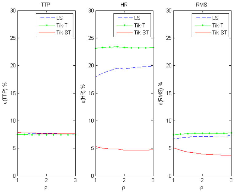
This simulation was designed to quantify the effects of smoothing the data with a Gaussian kernel and to assess the relative performance of the algorithm with spatio-temporal constraints versus Tikhonov-GCV-T and LS. The activation in all cases was simulated in the center of the image as shown in the left panel of figure 2. We analyze three situations: (a) the data are not smoothed and (b) the data are smoothed with a Gaussian isotropic kernel with full width half maximum (FWHM) of 2 pixels as a pre-processing step before using LS or Tik-GCV-T. These simulations are performed across different levels of Gaussian white noise (0.1–0.5 std). (c) The same as the previous one but we fixed the noise level (0.1 std) and we simulated a spatially varying activation profile. We used the Gaussian function , where x, y are the pixels coordinates and the pixel (x0, y0) lies at the center of the simulated circular activation in the left panel of figure 2. We experimented different widths of the Gaussian function by changing the parameter ρ given in the number of pixels.
Figure 2.

In the left and right panels the simulated activations used in simulations 1 and 2 are depicted. They contain 49 and 60 voxels, respectively.
Simulation 2
This simulation focuses on the performance of these methods exclusively at the edges. One activation is simulated on the edge of the region of interest (gray square) as shown in the right panel of figure 2. The boundary of the activation was determined. The HRFs and the measures of performance are computed only for the voxels lying on the boundary to quantify the impact of the edges on the HRF estimates by these methods. These simulations are performed across different levels of Gaussian white noise (0.1–0.5 std). The data were smoothed with a Gaussian isotropic kernel with full width half maximum (FWHM) of 2 pixels as a pre-processing step before using LS or Tik-GCV-T.
Simulation 3
These simulations were designed to compare the performance of the two regularization techniques in terms of the variability of the estimates. For four different ITImean values (3, 7, 10 and 15 s), the mean TTP and HR values, together with their 2.5% lower and upper tails, were computed for 200 realizations of the noise. Three different levels of white noise (0.1, 0.2 and 0.3 std) were explored. Other parameters in this simulation were TR = 1 s and temporal estimation resolution TR. The data were smoothed with a Gaussian isotropic kernel with full width half maximum (FWHM) of 2 pixels as a previous step before using LS or Tik-GCV-T.
Real data
Stimulus presentation
A healthy volunteer (47 year old male) provided written consent for MRI scanning. The subject was instructed to maintain fixation on a gray cross in the center of a projection screen and to concentrate on the visual stimulus, a black and white checkerboard (250 ms duration) that encompassed ~3° of visual space displayed using MR-compatible goggles (Resonance Technology, www.mrivideo.com). The subject was instructed to respond as quickly and as accurately as possible to the occurrence of a single flash of the checkerboard using the right index finger on a keypad. The single event-related paradigm used a geometric design optimized in terms of efficiency (Dale 1999) among 10 000 events generated at random. It consisted of 78 events totaling 330.8 s. The ITImin was 1.7 s, and there were null events built into the paradigm (p = 0.5) (Burock et al 1998).
Image acquisition
The experiment was conducted on a 1.5-T GE Twin-speed MRI scanner with EXCITE technology (GE Medical Systems, Milwaukee, WI). Functional imaging was performed in the axial plane using multi-slice gradient echo-planar imaging with a field of view of 24 cm (frequency) × 15 cm (phase) and an acquisition matrix of 64 × 40 (28 slices, 5 mm thickness, no gap, TR/TE = 2100 ms/40 ms, flip angle = 90°). A high-resolution structural image was obtained using a 3D spoiled gradient-echo sequence with matrix, 256 × 256; field of view, 24 cm; section thickness, 3 mm with no gap between sections; the number of sections, 128; and in-plane resolution, 0.94 mm.
Image Processing
Images were motion corrected within SPM99, normalized to Montreal Neurological Institute space using image header information (Maldjian et al 1997) combined with the SPM99 normalization, and resampled to 4 × 4 × 5 mm using sinc interpolation. Statistical parametric maps were generated using SPM99 from the Wellcome Department of Cognitive Neurology, London, England, and implemented in Matlab (The Mathworks Inc., Sherborn, MA) with an IDL (Research Systems Inc., Boulder, CO) interface. The data sets were smoothed using an 8 × 8 × 10 mm full-width-half-maximum Gaussian kernel. The data were high-pass filtered, detrended and globally normalized using the corresponding options in the SPM estimation module. Regional activity was detected using SPM by fitting a regression model based on the stimulus time series convolved with the canonical HRF and the first derivative. The SPMs were thresholded at uncorrected p < 0.000 01 and corrected for multiple comparisons using the random field theory functions for family wise error rate (cluster size test p < 0.05 corrected). The significantly activated region of the visual cortex containing 371 voxels was selected to carry out the HRF estimation. The SPM pre-processed data (without high pass filtering and global normalization) were fed to a set of MATLAB programs with our implementation of the different regularized HRF estimation techniques. The detrending of the time series was carried out as part of the estimation process as shown in equation (2) by including the polynomial term. No high-pass filtering or global normalization was applied. When Tik-GCV-T was applied the data were smoothed with the Gaussian kernel described above. The time span was fixed to 21 s. To obtain full brain coverage in this data set a relatively long TR (2.1 s) was used. We employ a time resolution of TR/4 to estimate the HRF. We have shown before (Casanova et al 2008) that LS performs worse than Tik-GCV-T when a time resolution finer than TR is used for HRF estimation. Therefore we do not present results for real data with LS. The computer used in all analyzes was a dual-core AMD processor system running at 3 GHz with 8 GB of RAM and 64 bit Redhat Linux OS.
Results and discussion
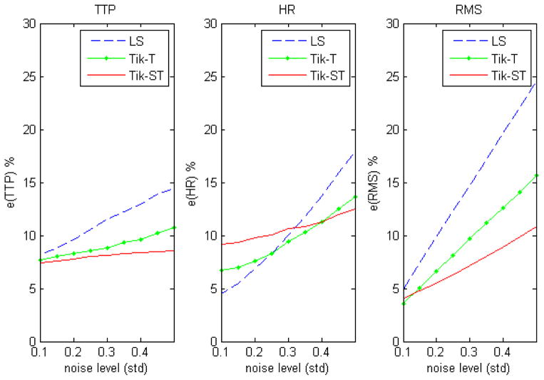
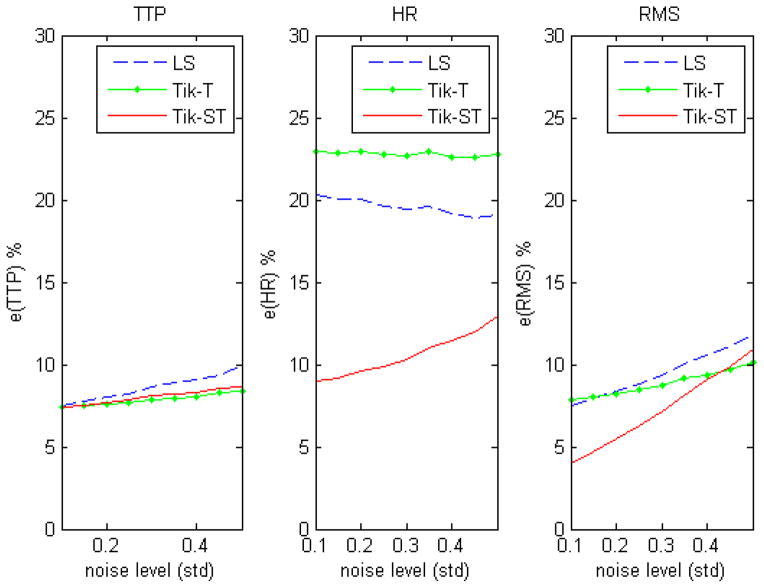
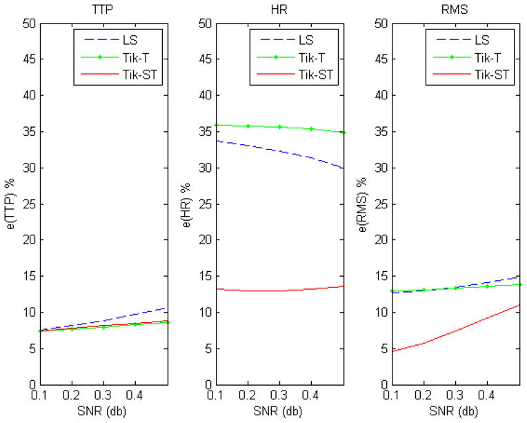
Comparisons of simulations across different noise levels using non-smoothed data are shown in figure 3. Tikhonov-GCV-ST is more accurate than the other two methods for all measures except for HR when the signal-to-noise ratio is high. Figure 4 shows the results of the same simulations for the situation when the data are smoothed with a Gaussian kernel prior to using LS and Tik-GCV-T. In this case, the estimation accuracy of these three methods comes closer in terms of the TTP and mean square errors measures (equations (7, 9)) though Tik-GCV-ST produces more accurate estimates of the response amplitude. In fact, in this last case, the Gaussian smoothing decreases the quality of the amplitude estimates. These results suggest that the smoothing introduced by spatial regularization is less severe than that resulting from the isotropic Gaussian kernel. Figure 5 shows the results for a spatially varying activation profile introduced by using a Gaussian function for a fixed level of white noise (0.1 std). We observe a very similar qualitative result as before. Tik-GCV-ST produces better estimates of the amplitude and the HRF time course in general.
Figure 3.
Results for unsmoothed data. In general Tikhonov-GCV-ST produces more accurate estimates of the HRF across the activated region.
Figure 4.
The spatio-temporal estimates of the HRF time course metrics are compared with the estimates produced by LS and Tik-GCV-T preceded by the application of a Gaussian filter. We recall the reader that no filtering of the data is applied when Tik-GCV-ST is used. The TTP estimates produced by Tikhonov-GCV-T are very similar to those generated by its spatio-temporal counterpart. However, the estimates of the response amplitude are more accurate with Tik-GCV-ST.
Figure 5.
The signal-to-noise ratio was fixed at 0.1 std and a spatially varying activation profile was simulated using a Gaussian function. Different widths of the Gaussian were tested by changing the parameter ρ. Again Tik-GCV-ST produces better estimates of the HRF response amplitude and the time course.
Figure 6 shows the results of simulations that quantify the difference in performance of the three methods when estimating the HRF at the edges for 100 realizations of the noise and across different signal-to-noise ratios (0.1–0.5 std). The spatio-temporal method produces similar estimates of TTP and is often more accurate when estimating the HRF amplitude. The results of the simulation 3 showed a very similar performance of the two regularization techniques in terms of bias and variability when estimating the TTP. However the estimates of the response amplitude were less biased and variable when the Tik-GCV-ST is used. We did not observe major differences of the time course metrics estimates across the different inter trial intervals (3, 7, 10 and 15 s) of the random designs.
Figure 6.
Measures of performance computed at the edge of the activation. As expected, the difference in performance when estimating the response amplitude is even greater than in the absence of an edge (see figure 4).
Real data results
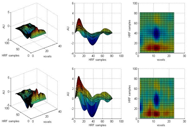
In figure 7, an activated region of the visual cortex is superimposed on the corresponding anatomical slice. A horizontal row crossing the activation is highlighted. HRFs across voxels lying in this row were estimated using both regularization methods. Figure 8 illustrates different three-dimensional views of the estimated HRFs using Tik-GCV-T (top row) and Tik-GCV-ST (bottom row) for the voxels along the horizontal row highlighted in figure 7. In both cases, 40 s of the HRF time course has been estimated. Though the spatio-temporal method produces a rougher image, a very good synchronization of the time to peaks is observed. Tik-GCV-ST also produces estimates with a higher amplitude than Tik-GCV-T, potentially increasing the sensitivity of this technique.
Figure 7.
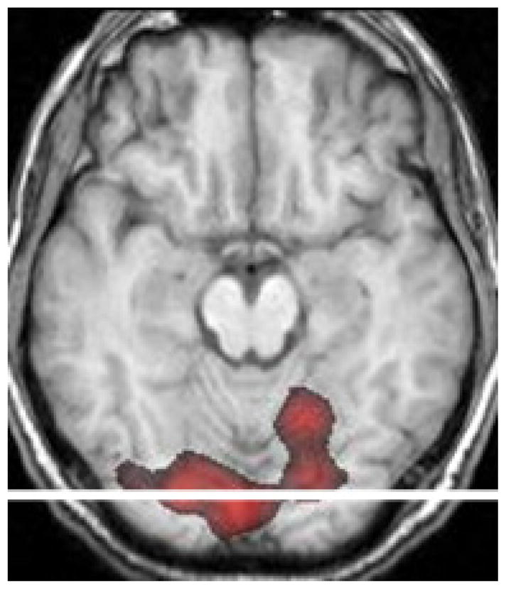
An activated region in the visual cortex is overlaid on the corresponding anatomical slice. A row crossing the activation horizontally is highlighted.
Figure 8.
Different views of the estimated HRFs by Tik-GCV-T (top row) and Tik-GCV-ST (bottom row), respectively, across the horizontal line shown in figure 8. Both methods produce well-synchronized time to peaks. However, the spatio-temporal method estimates higher response amplitudes.
It should be mentioned that the spatio-temporal algorithm is much slower than its temporal counterpart, due to the increased scale of the regression problem to be solved. In a whole brain computational experiment using the same real data set that contains around 23 000 voxels, Tik-GCV-T can be performed in less than 3 min while Tik-GCV-ST did the same task in 41 min.
Conclusions
In this work, we have proposed a new method based on Tikhonov regularization which estimates the BOLD fMRI hemodynamic response function with spatio-temporal smoothness constraints. This method does not require smoothing the data with a Gaussian filter; instead the smoothness is introduced by the spatial regularization. We have studied its relative performance in relation to its temporal version through two-dimensional simulations. The effect of data smoothing was analyzed, and we found that when the data are not smoothed the spatio-temporal method often produces more accurate estimates of the HRF according to all measures. Although smoothing the data with a Gaussian kernel causes the performance of the two algorithms to be more similar in terms of estimated TTP, it produces less accurate estimates of the HRF amplitude when used as a previous step to Tik-GCV-T. Simulations performed only on the edges of the simulated brain and activations show that these differences, as expected, are even greater in those areas. We observed in both simulations and real data analysis that both algorithms produced robust estimates of the TTP across the activated regions, suggesting the possibility of generating robust TTP maps. In terms of variability of the estimates, both methods show very similar performance when estimating TTP but the spatio-temporal algorithm shows less variability and bias when estimating the response amplitude.
The spatio-temporal method was much more time consuming, although in the simulated situations (single event related designs) it was feasible. However, the performance of the latter could be improved by using more sophisticated matrix computation algorithms that take advantage of the structure of these matrices (sparsity, blocks, etc), coding in C or FORTRAN or distributed computing, which will be pursued in a future study.
In this work, we assumed the noise to be Gaussian and i.i.d. or that an efficient pre-whitening procedure is available to be applied as a previous step. A thorough simulation study will be performed in the future to evaluate the impact of the fMRI data spatio-temporal correlation structure on the Tik-GCV-ST HRF estimates. The spatial smoothness constraint used here is two dimensional, similar to that used by Penny et al (2005) although fMRI is intrinsically a 3D process. The method can be expanded to three dimensions by using a 6-neighborhood system (Pascual-Marqui et al 1994) or more complex neighborhood systems. However, the performance of the method in its current 2D form for some specific situations is not known, such as when an activation is located in a plane perpendicular to that of the 2D estimation or when the inherent fMRI activation is not smooth temporally. These can arise for example, in some fMRI paradigms involving speech (Birn et al 1999) or when one is interested in examining BOLD activation in the sub-thalamic nucleus (a small structure) whose spatial extent may not involve more than a few voxels. Finally, a shortcoming of our Tikhonov-regularization-based methods is that in contrast to their Bayesian counterparts (Ciuciu et al 2003, Marrelec et al 2003, Woolrich et al 2004), they lack a signal detection scheme. So far we have relied on them to study HRF estimation properties in simulations or, for real data, we have used SPM software to detect activations before estimating the HRF. The development of detection methods will be the focus of future research.
Acknowledgments
This work was supported by the Human Brain Project and NIBIB through grant number EB004673, and by NS042568, and EB003880. We are grateful to the anonymous reviewers for their suggestions and comments that helped to improve this work significantly.
Appendix. Description of matrices L2 and
These matrices are illustrated for the case of voxels with four neighbors and Ns = 12. In all cases the dimension is (Ns − 2) × ((Ns − 2) (Nn + 1)).
Footnotes
Some figures in this article are in colour only in the electronic version
References
- Birn RM, Bandettini PA, Cox RW, Shaker R. Event-related fMRI of tasks involving brief motion. Hum Brain Mapp. 1999;7:106–14. doi: 10.1002/(SICI)1097-0193(1999)7:2<106::AID-HBM4>3.0.CO;2-O. [DOI] [PMC free article] [PubMed] [Google Scholar]
- Bonakdarpour B, Parrish TB, Thompson CK. Hemodynamic response function in patients with stroke-induced aphasia: implications for fMRI data analysis. Neuroimage. 2007;36:322–31. doi: 10.1016/j.neuroimage.2007.02.035. [DOI] [PMC free article] [PubMed] [Google Scholar]
- Boynton GM, Engel SA, Glover GH, Heeger DJ. Linear systems analysis of functional magnetic resonance imaging in human V1. J Neurosci. 1996;16:4207–21. doi: 10.1523/JNEUROSCI.16-13-04207.1996. [DOI] [PMC free article] [PubMed] [Google Scholar]
- Bullmore E, Long C, Suckling J, Fadili J, Calvert G, Zelaya F, Carpenter TA, Brammer M. Colored noise and computational inference in neurophysiological (fMRI) time series analysis: resampling methods in time and wavelet domains. Hum Brain Mapp. 2001;12:61–78. doi: 10.1002/1097-0193(200102)12:2<61::AID-HBM1004>3.0.CO;2-W. [DOI] [PMC free article] [PubMed] [Google Scholar]
- Burock MA, Buckner RL, Woldorff MG, Rosen BR, Dale AM. Randomized event-related experimental designs allow for extremely rapid presentation rates using functional MRI. Neuroreport. 1998;9:3735–9. doi: 10.1097/00001756-199811160-00030. [DOI] [PubMed] [Google Scholar]
- Carew JD, Wahba G, Xie X, Nordheim EV, Meyerand ME. Optimal spline smoothing of fMRI time series by generalized cross-validation. Neuroimage. 2003;18:950–61. doi: 10.1016/s1053-8119(03)00013-2. [DOI] [PubMed] [Google Scholar]
- Casanova R, Ryali S, Serences J, Yang L, Kraft R, Laurienti PJ, Maldjian JA. The impact of temporal regularization on estimates of the BOLD hemodynamic response function: a comparative analysis. Neuroimage. 2008;40:1606–18. doi: 10.1016/j.neuroimage.2008.01.011. [DOI] [PMC free article] [PubMed] [Google Scholar]
- Ciuciu P, Poline JB, Marrelec G, Idier J, Pallier C, Benali H. Unsupervised robust nonparametric estimation of the hemodynamic response function for any fMRI experiment. IEEE Trans Med Imaging. 2003;22:1235–51. doi: 10.1109/TMI.2003.817759. [DOI] [PubMed] [Google Scholar]
- Dale A. Optimal experimental design for event-related fMRI. Hum Brain Mapp. 1999;8:109–14. doi: 10.1002/(SICI)1097-0193(1999)8:2/3<109::AID-HBM7>3.0.CO;2-W. [DOI] [PMC free article] [PubMed] [Google Scholar]
- Dale A, Buckner RL. Selected averaging of rapidly presented individual trials using fMRI. Hum Brain Mapp. 1997;5:329–40. doi: 10.1002/(SICI)1097-0193(1997)5:5<329::AID-HBM1>3.0.CO;2-5. [DOI] [PubMed] [Google Scholar]
- Friston KJ, Holmes AP, Worsley KJ, Poline J-B, Frith C, Frackowiak RSJ. Statistical parametric maps in functional imaging: a general linear approach. Hum Brain Mapp. 1995;2:189–202. [Google Scholar]
- Friston KJ, Jezzard P, Turner R. Analysis of functional MRI time series. Hum Brain Mapp. 1994;1:153–71. [Google Scholar]
- Friston KJ, Mechelli A, Turner R, Price CJ. Nonlinear responses in fMRI: the Balloon model, Volterra kernels, and other hemodynamics. Neuroimage. 2000;12:466–77. doi: 10.1006/nimg.2000.0630. [DOI] [PubMed] [Google Scholar]
- Fuhrmann Alpert G, Sun FT, Handwerker D, D’Esposito M, Knight RT. Spatio-temporal information analysis of event-related BOLD responses. Neuroimage. 2007;34:1545–61. doi: 10.1016/j.neuroimage.2006.10.020. [DOI] [PMC free article] [PubMed] [Google Scholar]
- Golub GH, Heath M, Wahba G. Generalized cross-validation as a method for choosing a good ridge parameter. Technometrics. 1979;21:215–23. [Google Scholar]
- Goutte C, Nielsen FA, Hansen LK. Modeling the haemodynamic response in fMRI using smooth FIR filters. IEEE Trans Med Imaging. 2000;19:1188–201. doi: 10.1109/42.897811. [DOI] [PubMed] [Google Scholar]
- Hansen PC. Regularization tools: a Matlab package for analysis and solution of discrete ill-posed problems. Numer Algorithms. 1994;6:1–35. [Google Scholar]
- Lange N, Strother SC, Anderson JR, Nielsen FA, Holmes AP, Kolenda T, Savoy R, Hansen LK. Plurality and resemblance in fMRI data analysis. Neuroimage. 1999;10(3 Pt 1):282–303. doi: 10.1006/nimg.1999.0472. [DOI] [PubMed] [Google Scholar]
- Liu TT, Frank LR, Wong EC, Buxton RB. Detection power, estimation efficiency and predictability in event-related fMRI. Neuroimage. 2001;13:759–73. doi: 10.1006/nimg.2000.0728. [DOI] [PubMed] [Google Scholar]
- Lu Y, Bagshaw AP, Grova C, Kobayashi E, Dubeau F, Gotman J. Using voxel-specific hemodynamic response function in EEG-fMRI data analysis. Neuroimage. 2006;32:238–47. doi: 10.1016/j.neuroimage.2005.11.040. [DOI] [PubMed] [Google Scholar]
- Maldjian JA, Schulder M, Liu WC, Mun IK, Hirschorn D, Murthy R, Carmel P, Kalnin A. Intraoperative functional MRI using a real-time neurosurgical navigation system. J Comput Assist Tomogr. 1997;21:910–2. doi: 10.1097/00004728-199711000-00013. [DOI] [PubMed] [Google Scholar]
- Marrelec G, Benali H, Ciuciu P, Pelegrini-Issac M, Poline J-B. Robust estimation of the hemodynamic response function in event-related BOLD fMRI using basic physiological information. Hum Brain Mapp. 2003;19:1–17. doi: 10.1002/hbm.10100. [DOI] [PMC free article] [PubMed] [Google Scholar]
- Menon RS, Luknowsky DC, Gati JS. Mental chronometry using latency-resolved functional MRI. Proc Natl Acad Sci USA. 1998;95:10902–7. doi: 10.1073/pnas.95.18.10902. [DOI] [PMC free article] [PubMed] [Google Scholar]
- Miezin FM, Maccotta L, Ollinger JM, Petersen SE, Buckner RL. Characterizing the hemodynamic response: effects of presentation rate, sampling procedure, and the possibility of ordering brain activity based on relative timing. Neuroimage. 2000;11:735–59. doi: 10.1006/nimg.2000.0568. [DOI] [PubMed] [Google Scholar]
- Ogawa S, Lee TM, Kay AR, Tank DW. Brain magnetic resonance imaging with contrast dependent on blood oxygenation. Proc Natl Acad Sci USA. 1990;87:9868–72. doi: 10.1073/pnas.87.24.9868. [DOI] [PMC free article] [PubMed] [Google Scholar]
- Pascual-Marqui RD, Michel CM, Lehmann D. Low resolution electromagnetic tomography: a new method for localizing electrical activity in the brain. Int J Psychophysiol. 1994;18:49–65. doi: 10.1016/0167-8760(84)90014-x. [DOI] [PubMed] [Google Scholar]
- Penny WD, Trujillo-Barreto NJ, Friston KJ. Bayesian fMRI time series analysis with spatial priors. Neuroimage. 2005;24:350–62. doi: 10.1016/j.neuroimage.2004.08.034. [DOI] [PubMed] [Google Scholar]
- Serences JT. A comparison of methods for characterizing the event related BOLD time series in rapid fMRI. Neuroimage. 2004;21:1690–700. doi: 10.1016/j.neuroimage.2003.12.021. [DOI] [PubMed] [Google Scholar]
- Vakorin VA, Borowsky R, Sarty GE. Characterizing the functional MRI response using Tikhonov regularization. Stat Med. 2007;26:3830–44. doi: 10.1002/sim.2981. [DOI] [PubMed] [Google Scholar]
- Wahba G. Spline Models for Observational Data. Philadelphia: SIAM; 1990. [Google Scholar]
- Woolrich MW, Behrens TE, Smith SM. Constrained linear basis sets for HRF modelling using variational Bayes. Neuroimage. 2004;21:1748–61. doi: 10.1016/j.neuroimage.2003.12.024. [DOI] [PubMed] [Google Scholar]
- Worsley KJ, Liao CH, Aston J, Petre V, Duncan GH, Morales F, Evans A. A general statistical analysis for fMRI data. Neuroimage. 2002;15:1–15. doi: 10.1006/nimg.2001.0933. [DOI] [PubMed] [Google Scholar]
- Zhang CM, Jiang Y, Yu T. A comparative study of one-level and two-level semiparametric estimation of hemodynamic response function for fMRI data. Stat Med. 2007;26:3845–61. doi: 10.1002/sim.2936. [DOI] [PubMed] [Google Scholar]


