Statistical tests for measures of colocalization in biological microscopy

Summary

Colocalization analysis is the most common technique used for quantitative analysis of fluorescence microscopy images. Several metrics have been developed for measuring the colocalization of two probes, including Pearson's correlation coefficient (PCC) and Manders' correlation coefficient (MCC). However, once measured, the meaning of these measurements can be unclear; interpreting PCC or MCC values requires the ability to evaluate the significance of a particular measurement, or the significance of the difference between two sets of measurements. In previous work, we showed how spatial autocorrelation confounds randomization techniques commonly used for statistical analysis of colocalization data. Here we use computer simulations of biological images to show that the Student's one-sample t-test can be used to test the significance of PCC or MCC measurements of colocalization, and the Student's two-sample t-test can be used to test the significance of the difference between measurements obtained under different experimental conditions.

Introduction

Fluorescence microscopy is one of the most widely used tools in biomedical research, where it is used to determine the cellular and subcellular localization of biological molecules. In general, this involves a process in which the distribution of a fluorescent probe targeting a particular molecule is compared to that of a second fluorescent probe that labels a specific population of cells or subcellular compartment. Images of cells labelled with both probes are collected and evaluated for the degree of ‘colocalization’ of the two probes, and interpreted in terms of the function of the molecule. Colocalization is often evaluated subjectively; for example, one protein is labelled with a probe that fluoresces red, a second molecule is labelled with a probe that fluoresces green and colocalization of the two is visually identified in the regions of the image that appear yellow. If most of an image consists of yellow areas (where both proteins are present) on a black background (where both proteins are absent), the two proteins are clearly colocalized and no statistical analysis is necessary. As an example, Figure 1 shows cells that were incubated with both TexasRed-transferrin (red) and Cy5-transferrin (green). Because both probes interact with the same transferrin receptor, we would expect to see a high degree of colocalization between the two. Indeed, the degree of overlap is so complete that the case for colocalization of the two probes is convincing even in the absence of a statistical analysis.

Fig 1.

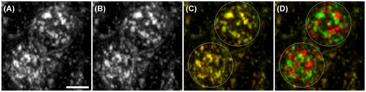
Living PTR cells incubated with TexasRed-transferrin (A) and Cy5-transferrin (B). Both probes bind to the transferrin receptor at the surface of cells, from which they are internalized into early endosomes. The extensive colocalization of the two is shown in panel C, which shows the two images merged together (red, TexasRed; green, Cy5). Panel D: the same image shown in panel C, after 90° rotation of the red image in each of the indicated regions. Scale bar indicates length of 10 μm.

However, this situation is uncommon; more often colocalization is less obvious than this, so that subjective evaluations are inconclusive. It would therefore be desirable to have a statistical test to help decide whether two proteins are colocalized. This requires two things: a statistical measure of colocalization, and knowledge of the distribution of that measure when the null hypothesis (that the proteins are not colocalized) is true. If the observed value of the colocalization statistic is unlikely under the null hypothesis, then the null hypothesis is rejected and the alternative hypothesis, that the two proteins are colocalized, is accepted. There are currently two widely accepted statistical measures of colocalization – Pearson's correlation coefficient (PCC) and Manders' colocalization coefficient (MCC) (Manders et al., 1993).

In PCC analyses, each pixel is considered one data point, and the intensity of the red signal and green signal is measured at each pixel. The correlation coefficient is then measured across all pixels in the area of interest in an image. PCC values range from −1 to +1, and they are simple to interpret. If there is no association between the proteins, the expected PCC is 0. A positive PCC means the two proteins are colocalized to some extent; higher values of red are associated with higher values of green. And a negative PCC value indicates that the distributions of the two probes are inversely related, with higher red values being associated with lower green values; for example, if one protein is restricted to the cell nucleus, and a second is localized in the cell cytosol.

When N data points are statistically independent of each other, the significance of a PCC value is tested by calculating t = PCC √([N − 2]/[1 − PCC²]), which is t-distributed with N − 2 degrees of freedom (Fisher, 1915; McDonald, 2009, pp. 207–220). However, in images of cells, the pixels are not statistically independent data points. Instead, they are autocorrelated, meaning that each pixel is likely to have similar values to its neighbouring pixels. This autocorrelation occurs for two reasons. The first source of autocorrelation is the point-spread function of the imaging system, which spreads the signal of a point source to several adjacent pixels in a properly designed imaging system. The second source of autocorrelation is the subcellular structure of the cell itself. The size of subcellular structures is such that their images typically occupy a large number of pixels. Thus, if the probe fluorescence is strong in one pixel in the image of the structure, it is also likely to be strong in the adjacent pixels as well. It has long been known that autocorrelation causes the expected distribution of PCC under the null hypothesis to be much broader than if the same number of data points were independent (Student, 1914). Using the usual test of a PCC value for an image that is 200 × 200 pixels (39 998 degrees of freedom), any PCC greater than 0.01 or less than −0.01 would be significant at the p < 0.05 level. When tested using this inappropriate method, simulated data with no real colocalization can yield a ‘significant’ (p < 0.05) result almost all of the time. For example, Figure 1D shows images of the cells that were incubated with both TexasRed-transferrin (red) and Cy5-transferrin (green) after rotating a circular region of the red channel by 90°, a procedure that would result in random overlap between the two channels. Even though this randomization should produce no real correlation between red and green values, PCC values in each cell are 0.17, which is highly significant under the usual significance test for PCC. In simulated 200 × 200 pixel images with red and green circular ‘objects’ positioned randomly, almost all of the images have PCC values greater than 0.01 or less than −0.01 (Fig. 2), which could mislead an investigator into thinking that there was significant colocalization or anticolocalization between almost any pair of proteins in a cell.

Fig 2.

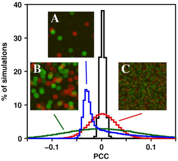
Distribution of PCC values for simulated images with different amounts of autocorrelation. Blue line, images with high autocorrelation and a small number of objects (5 red and 5 green objects, diameter 21 pixels, example image A); green line, images with high autocorrelation and a larger number of objects (50 red and 50 green objects, diameter 21 pixels, example image B); red line, images with moderate autocorrelation (1000 red and 1000 green objects, diameter 5 pixels, example image C); black line, images with no autocorrelation (each pixel with a random red and green value, no PSF applied).

In one approach that has been developed to test the significance of a colocalization measurement, the probability of obtaining a particular measurement is estimated based upon a distribution of values measured for ‘randomized’ data, in which colocalization is measured between images after one has been shifted relative to the other (van Steensel et al., 1996; Fay et al., 1997; Ramírez et al., 2010) or between images from different regions in the image (Lachmanovich et al., 2003). In practice, it is frequently difficult to obtain enough mismatched image regions to generate a useful random distribution. In a second approach, the probability of obtaining a particular measurement is estimated based upon a distribution of values measured after one of the images has been divided into blocks of pixels, which are then randomly distributed (Costes et al., 2004). We have previously shown that this approach can spuriously indicate colocalization even in random data, as it reduces autocorrelation in the scrambled images, resulting in ‘randomized’ data with far too many low correlation values (Dunn et al., 2011).

Here we describe a much more straightforward method for testing the significance of PCC and MCC values measured in colocalization studies. In studies of simulated data and in examples of biological image data, we show how deriving estimates of variability from the measured variates themselves can be used to reliably estimate probability values, which in turn can be used to evaluate the significance of colocalization measurements. We also show that the two-sample t-test (McDonald, 2009, pp. 118–122) can be used to compare measurements of colocalization, an approach that has been previously used (Wang et al., 2001; Babbey et al., 2006; Rondanino et al., 2007; Khandelwal et al., 2008), but without consideration of possible statistical artefacts. Here we use simulated data to show that the two sample t-test and the paired t-test give accurate results across a variety of conditions.

Materials and methods

Simulation procedures

To test the accuracy of the one-sample t-test, a Pascal computer program was written to simulate a square image, 200 by 200 pixels, with two colours, red and green. The image was divided into background and objects. Background pixels were given greyscale values of red and green chosen from a uniform random distribution ranging from 0 to 1000, to simulate the noise inherent in imaging (e.g. shot noise and detector noise). Circular objects were then added to the background, with a maximum value for each object chosen from a uniform random distribution ranging from 1000 to 4095 (the maximum greyscale value in a 12-bit image). The value of each pixel within an object was chosen from a uniform random distribution ranging from 1000 to the maximum value for the object. The number and size of the objects was varied to test the performance of the one-sample t-test under different conditions. The centre of each object was positioned at random in the image; if this would make the object extend past the edge of the image, the object was wrapped around to the other side. Red and green objects were positioned independently to simulate the null hypothesis of no colocalization. After the initial greyscale values of the pixels were determined, a Gaussian point spread function was applied using a kernel of 9 by 9 pixels and a standard deviation of 2. Examples of simulated images are shown in Figures 2 and 3A.

Fig 3.

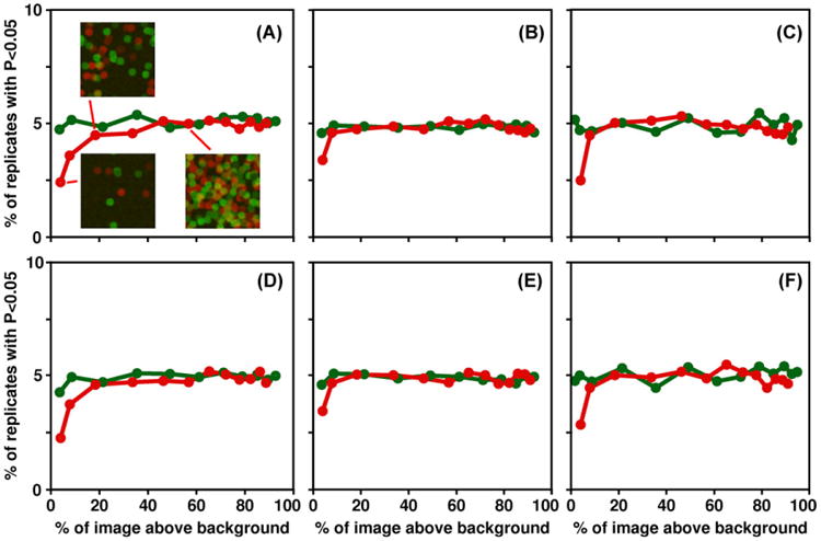
Percentage of simulated images with p values less than 0.05 for three statistical tests: one-sample t-test (A and D), two-sample t-test (B and E) and paired t-test (C and F). Results for PCC are on the top row, MCC_diff on the bottom row. Red lines are objects with a diameter of 21 pixels, green lines a diameter of 5 pixels; the number of objects was varied to produce images with different percentages of the image above the background threshold. Examples of images with 5, 25 and 100 objects of each color, diameter 21 pixels, are shown in A.

For each image, PCC (McDonald, 2009, pp. 207–220) was calculated between the greyscale values of the red and green channels. The PCC was calculated for a set of six simulated images, to simulate imaging a sample of six different cells. The p value was calculated using a one-sample Student's t-test (Sokal & Rohlf, 2012, pp. 152–153) comparing the mean PCC for each set of images with the value of 0 expected if there were no colocalization. Because most studies are only interested in colocalization and would not test the significance of a negative correlation value, one-tailed tests (considering only positive mean PCC values) were done, and the proportion of simulated p values that were below 0.05 was counted over 10 000 replicate sets of images for each combination of object size and number of objects.

For each image, Mander's correlation coefficients MCC₁ and MCC₂ (Manders etal.,1993) were calculated, using a threshold between ‘present’ and ‘background’ of 1000 greyscale units. The expected MCC (proportion of green pixels above background for MCC₁, proportion of red pixels above background for MCC₂) was subtracted from the observed MCC to yield an MCC_diff for each image, and Student's one-sample t-test was used to compare the mean MCC_diff to 0.

To test the accuracy of the two-sample t-test, a second program was written that performed simulations as described above, except that PCC and MCC_diff values were calculated for two sets of six images. The significance of the difference in mean PCC or MCC_diff values was then calculated for each pair of image sets, and the proportion of simulated p values that were below 0.05 was counted over 10 000 replicate sets of images for each combination of sample size, object size and number of objects.

To test the accuracy of the paired t-test, a third program was written that performed simulations as described above, except that three colours (red, green and blue) were simulated for sets of six images. The red–green PCC was compared with the red–blue PCC using the paired t-test, and the proportion of simulated p values that were below 0.05 was counted over 10 000 replicate sets of images for each combination of sample size, object size and number of objects.

The source code for all three Pascal programs is available (Supplementary material).

Fluorescence microscopy studies

Microscopy studies were conducted using PTR cells, MDCK strain II cells transfected with both the human TfR and the rabbit pIgR, previously described (Brown et al., 2000). Transient expression of GFP–Rab10 and GFP–Rab10–Q68L, immunofluorescence localization of Rab11a and endocytic labelling with fluorescent transferrin were accomplished as previously described (Babbey et al., 2006). All experiments were conducted using a Perkin–Elmer Ultraview confocal microscope system mounted on a Nikon TE 2000U inverted microscope, using Nikon 60× NA 1.2 water immersion or Nikon 100×, NA 1.4 oil immersion planapochromatic objectives.

Digital image analysis

Image processing, including measurement of PCC was conducted using Metamorph software (Universal Imaging, West Chester, PA, U.S.A.). Images shown in figures were contrast stretched to enhance the visibility of dim structures, with specific care taken to ensure that dim objects were never deleted from an image. Montages were assembled and annotated using Photoshop (Adobe, Mountain View, CA, U.S.A.).

Results

Testing mean PCC measurements

The simulations calculate a PCC value for each of six images and use the one-tailed, one-sample t-test to see whether the mean PCC value is significantly greater than 0, and repeat this for 10 000 sets of six images. Because the simulated objects are placed randomly in the images, there is no real colocalization, so a p value less than 0.05 is a false positive. A well-behaved statistical test should give a p value less than 0.05 in about 5% of replicate simulations. The one-tailed, one-sample t-test behaves well; about 5% of the sets of simulated images give a false positive, for a broad range of number and size of objects (Fig. 3A). When there is a small number of objects, so that most of the image is background, the test is conservative; the percentage of false positives is less than 5%. We have done other simulations with other background levels, other object sizes, other numbers of images, and a difference between the numbers of red and green objects, and all yield a false positive rate of about 5% or less (results not shown).

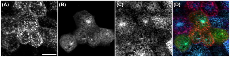
In Figure 1, we showed an example of a biological imaging study for which the colocalization of the two probes is so obvious that statistical analysis is unnecessary. In Figure 4, we show fluorescence microscopy images that are more typical of colocalization studies; the case for colocalization is less obvious, and a test of statistical significance would be useful.

Fig 4.

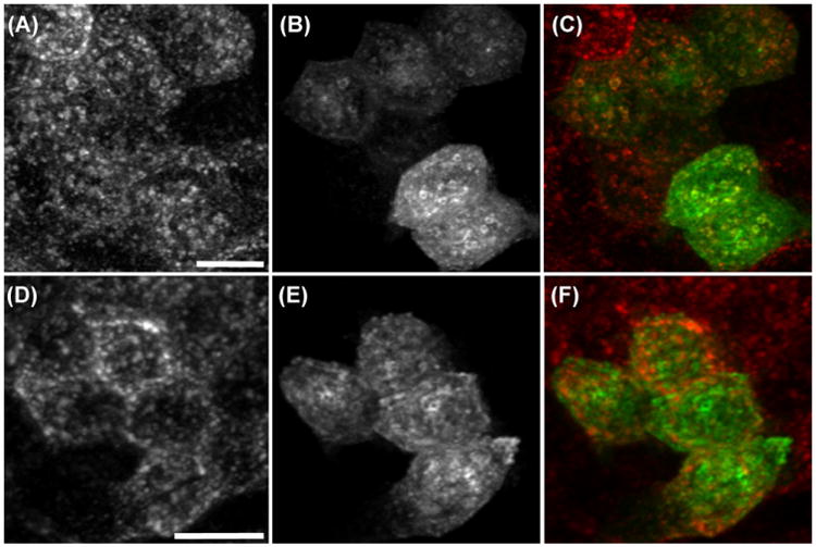
Studies of colocalization of endosomal proteins. (A) TexasRed-transferrin internalized into endosomes of a living PTR cell, transiently expressing GFP–Rab10 (B). (C) Merger of images shown in panels A and B (red, TexasRed; green, GFP). (D) TexasRed-transferrin internalized into endosomes of a living PTR cell, transiently expressing GFP–Rab10–Q68L (E). (F) Merger of images shown in panels D and E (red, TexasRed; green, GFP). Scale bars indicate length of 20 μm.

The top three panels show fluorescence microscopy images of the distribution of internalized TexasRed-transferrin (A) and GFP–Rab10 (B) in living, polarized PTR cells. Although careful examination reveals many examples of colocalization of the two probes, the degree of colocalization is unclear. The merger of the two images shown in panel C is no help; because of the disparity in signal levels of the two probes, very few of the endosomes take on the yellow colour reflecting the combination of red and green probes. For the five cells in this field, PCC measured 0.52, 0.20, 0.59, 0.62 and 0.60, suggesting some degree of colocalization of the two probes. The mean PCC is 0.51, a highly significant value according to a one-tailed t-test (t = 6.46, 4 d.f., p = 0.0015).

Most colocalization studies only consider positive PCC values to be of interest, so a one-tailed t-test is appropriate. If the investigator decides, before looking at the data, that either colocalization or anticolocalization would be interesting, then a two-tailed test should be used. It should be used with caution, however. As shown by the blue line in Figure 2, when there are a small number of objects, most images will have no overlapping objects and thus will have a slightly negative PCC, whereas a small number of images will include overlapping red and green objects and have a larger positive PCC. Under these conditions, testing a small number of images can result in more than 5% false positives (results not shown). When the probability is small that an image includes overlapping red and green images, a large number of images must be tested before concluding that there is significantly less overlap than predicted by the null hypothesis.

The bottom three panels of Figure 4 show fluorescence microscopy images of the distribution of TexasRed-transferrin (D) and anti-Rab11 antibody (E) in polarized PTR cells, with the merger of the two images shown in panel F. Unlike Rab10, Rab11 associates with an apical compartment that is inaccessible to transferrin (Brown et al., 2000; Babbey et al., 2006). Consistent with these previous studies, PCC analysis of the distributions of transferrin and Rab11 in 36 cells yields a mean PCC of −0.067. This mean PCC value is less than zero, which might suggest that transferrin is excluded from Rab11-containing compartments. However, the two-tailed t-test is not significant (t = 0.91, 19 d.f., p = 0.37), so the data fail to indicate either colocalization or anticolocalization between transferrin and Rab11a.

Testing the difference between PCC measurements

In order to evaluate whether colocalization measurements obtained from two samples (e.g. different cells, different pairs of proteins or different experimental conditions) differ significantly from one another, one uses a two-sample t-test to test the null hypothesis that that the mean PCC values are equal for two sets of cells. Simulations show that it gives accurate estimates of the p value across a broad range of conditions (Fig. 3B). It is some what conservative when there are very few objects and almost all of the image is background.

The use of the two-sample t-test to test the effect of a protein mutation is demonstrated with the following example. In previous studies of Rab10 (Babbey et al., 2006), we demonstrated that a single amino acid change (Q68L) altered the intracellular distribution such that Rab10 associated with apical recycling endosomes located at the top of PTR cells. This redistribution is apparent in a comparison of the association of GFP–Rab10 and transferrin, shown in Figure 4C, with the association of GFP–Rab10–Q68L and transferrin, shown in Figure 5A and B. GFP–Rab10 and transferrin have a mean PCC of 0.61, whereas GFP–Rab10–Q68L and transferrin have a mean PCC of 0.12. A two-sample t-test applied to test the hypothesis that the Q68L mutation reduces the colocalization of Rab10 with transferrin indicates a highly significant difference (t = 10.73, 50 d.f., p < 10⁻¹³).

Fig 5.

Studies of colocalization of endosomal proteins. Living PTR cells with endosomes labelled with TexasRed-transferrin (A), GFP–Rab10–Q68L (B) and Cy5-IgA (C). (D) Merger of images shown in panels A–C. Scale bar indicates length of 20 microns.

A potentially more powerful way to compare colocalization of A and B to the colocalization of A and C would be through a paired t-test (McDonald, 2009, pp. 191–197). In this case, cells would be labelled for all three proteins, and the PCC value for A with B is compared with the PCC value for A with C in each cell. By eliminating cell–cell variability from the comparison, this approach provides a more sensitive test of whether the mean difference in PCC values is significantly different from 0. The paired t-test has the null hypothesis that within each cell, the PCC value for A with B is equal to the PCC value for A with C. Like the two-sample t-test, it gives accurate estimates of the p value for most conditions, and is conservative when most of the image is background (Fig. 3C).

The application of the paired t-test is demonstrated in an evaluation of the redistribution of Rab10 induced by the Q68L mutation. As mentioned above, our previous studies indicated that the Q68L mutation induced a redistribution of Rab10 from endosomes containing transferrin to a population of apical recycling endosomes (Babbey et al., 2006). To test the hypothesis, cells were transfected with Rab10–Q68L, and incubated with both TexasRed-transferrin and Cy5-IgA, an endocytic ligand that labels the apical recycling endosomes. Consistent with our hypothesis, a paired t-test determined that Rab10–Q68L colocalizes significantly more with IgA than with transferrin (t = 17.02, 29 d.f., p < 10⁻¹²).

Statistical analyses of MCC

An alternative, commonly used metric for measuring colocalization is MCC, which provides a measure of the fraction of one probe that colocalizes with a second probe (Manders et al., 1993). Although providing a colocalization metric that some find easier to interpret than PCC, MCC analysis is more challenging, as it is very sensitive to the threshold separating objects from background, which can be difficult to assign (Dunn et al., 2011).

In terms of significance testing, MCC differs from PCC in that the expected MCC value under the null hypothesis of no colocalization will vary from cell to cell. For example, if 60% of the pixels in an image are above the threshold for the green probe, the expected fraction of the red probe that is colocal with A (MCC₁) is 0.60; one would expect 60% of the pixels with red signal to fall on pixels with green signal, if distributed randomly. This makes MCC values difficult to interpret in isolation: an MCC₁ of 0.60 would mean strong colocalization if only 5% of the image was green, no association if 60% of the image was green, and strong anticolocalization if 95% of the image was green. Evidence for colocalization or anticolocalization comes from the difference between the observed and expected MCC, not from MCC by itself. Thus, any statistical test must analyze the difference between the observed and expected MCC. We therefore use simulated images to determine whether the one-sample t-test, two-sample t-test and paired t-test can be used to test the significance of the difference between observed and expected MCC values (MCC_diff).

The results of simulations demonstrate that MCC_diff performs very similarly to PCC. One-tailed one-sample t-tests are accurate for most conditions, as the p value is less than 0.05 for about 5% of simulated images (Fig. 3D). When most of the image is background, the t-test is conservative: less than 5% of simulated images have a p value less than 0.05. The two-sample t-test and paired t-test of MCC_diff also give accurate estimates of the p value across a broad range of conditions (Figs. 3E and 3F). The similar results are not surprising as MCC_diff is highly correlated with PCC (Fig. 6).

Fig 6.

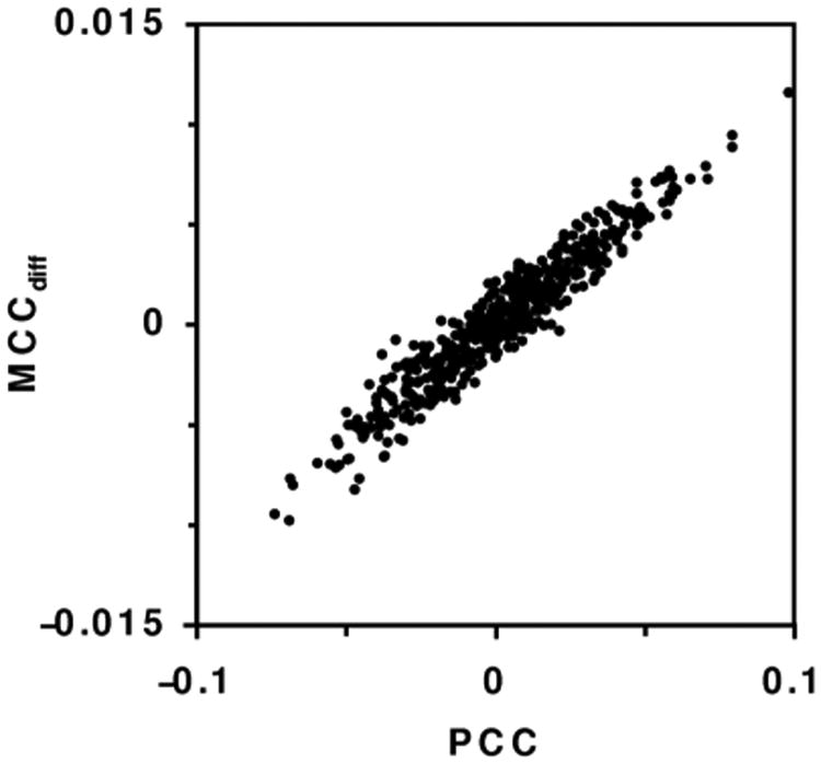
PCC and MCC_diff for 500 images with 1000 objects and object diameter 5 pixels.

Discussion

Both of the statistics considered here – PCC and MCC_diff – can be used as measures of colocalization in cell imaging studies. Here we have shown that the one-tailed, one-sample t-test is an effective method for statistically testing whether there is more association between two proteins than expected by chance. The PCC or MCC_diff is calculated for multiple images, and the t-test is used to test whether the mean value is significantly greater than zero. Our simulations show that if there is no actual colocalization, the t-test would give a false positive result (p < 0.05) about 5% or less of the time, as a well-behaved statistical test should.

Most biological uses of one-sample t-tests use the two-tailed p value, because a deviation from the null expectation in either direction would be interesting. For example, if one was studding asymmetry of arm length, one might use the one-sample t-test to see if the average ratio of right arm to left arm length was different from 1, and values of the right/left ratio that were either greater than one (indicating longer right arms) or less than one (longer left arms) could be important. In contrast, colocalization studies generally address the question of whether two molecules are colocal with each other, so a negative correlation value and zero correlation have the same interpretation, that there is no positive colocalization. This makes the one-tailed test appropriate for most colocalization studies. A one-tailed test is more powerful than a two-tailed test when there is positive correlation, and when the image is mostly background, a two-tailed test can yield an excessive number of false positives; using a one-tailed test avoids this artefact. In the rare cases where an investigator is interested in determining whether the distributions of two molecules are negatively correlated, either a one-tailed test that considers both positive and zero correlation values to be evidence of lack of anticolocalization, or a two-tailed test, can be used, but a large sample size and caution in interpreting the results are necessary due to the potential artefact caused by sparse objects.

Although MCC provides a measure of colocalization (fractional overlap) that some find more intuitively meaningful than PCC (fraction of variance in A explained by its linear relation with B), it is more difficult to use. Unlike PCC, MCC requires estimation of threshold values that discriminate signal from background, and MCC values vary wildly depending upon how this threshold is set (Dunn et al., 2011). Responsible use of MCC therefore requires an a priori, or at least consistent, criterion for assigning the threshold value. Costes et al. (2004) developed a method in which the threshold value is set at the lower limit of the range of pixel values in which a positive PCC value is obtained. This technique has been implemented in a variety of image processing software packages, and works well in many, but not all cases (Dunn et al., 2011).

It is important to keep in mind that a statistically significant result should not be considered sufficient evidence of colocalization by itself. A statistically significant association between red and green signals could result from crosstalk, uneven illumination or poor definition of the region of interest (such as including extracellular space) (Dunn et al., 2011). Careful microscopy and careful inspection of images and scatterplots are important before concluding that proteins are actually colocalized. On the other hand, failure to find a statistically significant colocalization measure is compelling evidence that any visually apparent colocalization is likely to result from wishful thinking.

In addition to testing the significance of a colocalization measurement, cell biologists often want to know whether the strength of colocalization changes under different conditions, or whether one pair of proteins is more strongly colocalized than another. For this the two-sample t-test works well, whether applied to the PCC or MCC_diff. It is not surprising that the two-sample t-test works well, as it is known to be robust to violations of normality and differences in variance (Lix et al., 1996) under most conditions. This robustness applies when the sample sizes are equal, as in the simulations done here. If the two sample sizes are markedly different, it is possible for the two-sample t-test to give ‘significant’ results much too often (Lix et al., 1996). Experimenters should therefore strive to have approximately the same number of cells for each sample when performing a two-sample t-test.

When colocalization can be measured between two pairs of proteins (such as A with B and A with C) in the same cell, a paired t-test may be more powerful than the two-sample t-test. This is especially true when the A–B colocalization and A–C colocalization vary widely among cells, but the difference between the A–B and A–C colocalization is consistent. Again, both PCC and MCC_diff perform well in paired t-tests.

We have described a simple method for statistically evaluating measures of colocalization used in biological microscopy. These methods take advantage of the fact that measures can be obtained from multiple cells, supporting estimation of sample variation from direct measurements. This situation contrasts with that found in other scientific domains, where the question of colocalization may need to be addressed in a single sample, such as in astronomy or ecology. Modifications to the usual test for PCC that correct for autocorrelation (Clifford et al., 1989; Dutilleul, 1993) have been applied to ecological studies to assess the association of different ecological variables (Fortin & Payette, 2002). We have conducted preliminary studies of simulated image data indicating that the approach of Clifford et al. (1989) provides reasonably accurate tests of significance in studies of cells. However, it is difficult to imagine a legitimate circumstance in which a single image would comprise a data set in biological microscopy; thus we have not included these results here.

One can imagine experiments in which more complicated statistical tests could be applied to measures of colocalization, such as analysis of variance (anova) and regression. Although we have not simulated the broad variety of possible experimental designs, our results here suggest that treating PCC or MCC_diff as a variable to be analyzed like any other measurement variable is a promising approach that may not suffer from obvious statistical artefacts.

References

- Babbey CM, Ahktar N, Wang E, Chen CCH, Grant BD, Dunn KW. Rab10 regulates membrane transport through early endosomes of polarized Madin–darby canine kidney cells. Molec Biol Cell. 2006;17:3156–3175. doi: 10.1091/mbc.E05-08-0799. [DOI] [PMC free article] [PubMed] [Google Scholar]
- Brown PS, Wang EX, Aroeti B, Chapin SJ, Mostov KE, Dunn KW. Definition of distinct compartments in polarized Madin– darby canine kidney (MDCK) cells for membrane-volume sorting, polarized sorting and apical recycling. Traffic. 2000;1:124–140. doi: 10.1034/j.1600-0854.2000.010205.x. [DOI] [PubMed] [Google Scholar]
- Clifford P, Richardson S, Hemon D. Assessing the significance of the correlation between 2 spatial processes. Biometrics. 1989;45:123–134. [PubMed] [Google Scholar]
- Costes SV, Daelemans D, Cho EH, Dobbin Z, Pavlakis G, Lockett S. Automatic and quantitative measurement of protein–protein colocalization in live cells. Biophys J. 2004;86:3993–4003. doi: 10.1529/biophysj.103.038422. [DOI] [PMC free article] [PubMed] [Google Scholar]
- Dunn KW, Kamocka MM, McDonald JH. A practical guide to evaluating colocalization in biological microscopy. Am J Physiol Cell Physiol. 2011;300:C723–C742. doi: 10.1152/ajpcell.00462.2010. [DOI] [PMC free article] [PubMed] [Google Scholar]
- Dutilleul P. Modifying the t-test for assessing the correlation between 2 spatial processes. Biometrics. 1993;49:305–314. [Google Scholar]
- Fay FS, Taneja KL, Shenoy S, Lifshitz L, Singer RH. Quantitative digital analysis of diffuse and concentrated nuclear distributions of nascent transcripts, SC35 and poly (A) Exp Cell Res. 1997;231:27–37. doi: 10.1006/excr.1996.3460. [DOI] [PubMed] [Google Scholar]
- Fisher RA. Frequency distribution of the values of the correlation coefficient in samples from an indefinitely large population. Biometrika. 1915;10:507–521. [Google Scholar]
- Fortin MJ, Payette S. How to test the significance of the relation between spatially autocorrelated data at the landscape scale: a case study using fire and forest maps. Ecoscience. 2002;9:213–218. [Google Scholar]
- Khandelwal P, Ruiz WG, Balestreire-Hawryluk E, Weisz OA, Gold-enring JR, Apodaca G. Rab11a-dependent exocytosis of discoidal/fusiform vesicles in bladder umbrella cells. Proc Natl Acad Sci USA. 2008;105:15773–15778. doi: 10.1073/pnas.0805636105. [DOI] [PMC free article] [PubMed] [Google Scholar]
- Lachmanovich E, Shvartsman DE, Malka Y, Botvin C, Henis YI, Weiss AM. Co-localization analysis of complex formation among membrane proteins by computerized fluorescence microscopy: application to immunofluorescence co-patching studies. J Microsc. 2003;212:122–131. doi: 10.1046/j.1365-2818.2003.01239.x. [DOI] [PubMed] [Google Scholar]
- Lix LM, Keselman JC, Keselman HJ. Consequences of assumption violations revisited: a quantitative review of alternatives to the one-way analysis of variance F test. Rev Educ Res. 1996;66:579–619. [Google Scholar]
- Manders EMM, Verbeek FJ, Aten JA. Measurement of colocalization of objects in dual-color confocal images. J Microsc. 1993;169:375–382. doi: 10.1111/j.1365-2818.1993.tb03313.x. [DOI] [PubMed] [Google Scholar]
- McDonald JH. Handbook of Biological Statistics. 2nd. Sparky House Publishing; Baltimore, Maryland: 2009. [Google Scholar]
- Ramírez O, García A, Rojas R, Couve A, Härtel S. Confined displacement algorithm determines true and random colocalization in fluorescence microscopy. J Microsc. 2010;239:173–183. doi: 10.1111/j.1365-2818.2010.03369.x. [DOI] [PubMed] [Google Scholar]
- Rondanino C, Rojas R, Ruiz WG, Wang E, Hughey RP, Dunn KW, Apodaca G. RhoB-dependent modulation of postendocytic traffic in polarized madin-darby canine kidney cells. Traffic. 2007;8:932–949. doi: 10.1111/j.1600-0854.2007.00575.x. [DOI] [PubMed] [Google Scholar]
- Sokal RR, Rohlf FJ. Biometry. 4th. W.H. Freeman; New York: 2012. [Google Scholar]
- Student. The elimination of spurious correlation due to position in time or space. Biometrika. 1914;10:179–181. [Google Scholar]
- van Steensel B, van Binnendijk EP, Hornsby CD, van der Voort HT, Krozowski ZS, de Kloet ER, van Driel R. Partial colocalization of glucocorticoid and mineralocorticoid receptors in discrete compartments in nuclei of rat hippocampus neurons. J Cell Sci. 1996;109:787–792. doi: 10.1242/jcs.109.4.787. [DOI] [PubMed] [Google Scholar]
- Wang EX, Pennington JG, Goldenring JR, Hunziker W, Dunn KW. Brefeldin A rapidly disrupts plasma membrane polarity by blocking polar sorting in common endosomes of MDCK cells. J Cell Sci. 2001;114:3309–3321. doi: 10.1242/jcs.114.18.3309. [DOI] [PubMed] [Google Scholar]
Associated Data
This section collects any data citations, data availability statements, or supplementary materials included in this article.