

Abstract
In this paper, we present a method based on Radial Basis Function (RBF)-generated Finite Differences (FD) for numerically solving diffusion and reaction-diffusion equations (PDEs) on closed surfaces embedded in ℝd. Our method uses a method-of-lines formulation, in which surface derivatives that appear in the PDEs are approximated locally using RBF interpolation. The method requires only scattered nodes representing the surface and normal vectors at those scattered nodes. All computations use only extrinsic coordinates, thereby avoiding coordinate distortions and singularities. We also present an optimization procedure that allows for the stabilization of the discrete differential operators generated by our RBF-FD method by selecting shape parameters for each stencil that correspond to a global target condition number. We show the convergence of our method on two surfaces for different stencil sizes, and present applications to nonlinear PDEs simulated both on implicit/parametric surfaces and more general surfaces represented by point clouds.
Keywords: radial basis functions, finite differences, mesh-free, manifolds, RBF-FD, method-of-lines, reaction-diffusion
1 Introduction
Methods based on global Radial Basis Functions (RBFs) have become quite popular for the numerical solution of the partial differential equations (PDEs) due to their ability to handle scattered node layouts, their simplicity of implementation and their spectral accuracy and convergence on smooth problems. While these methods have been successfully applied to the solution of PDEs on planar regions [10], they have also been applied to PDEs on the two-sphere
 (e.g. [13,14,25]).
Many methods have been developed for the solution of the class of PDEs known as diffusion (or reaction-diffusion) equations on more general surfaces. Of these, the so-called intrinsic methods attempt to solve PDEs using surface-based meshes and coordinates intrinsic to the surface under consideration; this approach can be efficient since the dimension of the discretization is restricted to the dimension of the surface under consideration (e.g. [3,9]). However, such intrinsic coordinates can contain singularities or distortions which are difficult to accomodate. A popular alernative is the class of so-called embedded, narrow-band methods that extend the PDE to the embedding space, construct differential operators in extrinsic coordinates, and then restrict them to a narrow band around the surface (e.g. [29, 30]). Such methods incur the additional expense of solving equations in the dimension of the embedding space; the curse of dimensionality will ensure these costs will grow rapidly depending on the order of accuracy of the method.
RBFs have recently been used to compute an approximation to the surface Laplacian in the context of a pseudospectral method for reaction-diffusion equations on manifolds [23]. In that study, global RBF interpolants were used to approximate the surface Laplacian at a set of “scattered” nodes on a given surface, combining the advantages of intrinsic methods with those of the embedded methods. This method showed very high rates of convergence on smooth problems on parametrically and implicitly defined manifolds. However, for N points on the surface, the cost of that method scales as O(N3). Furthermore, the dense nature of the resulting differentiation matrices means that the cost of applying those matrices to solution vectors is O(N2), assuming the manifold is static. Our goal is to develop a method that is less costly to apply than the global RBF method while still retaining the ability to use scattered nodes on the surface to approximate derivatives, thereby combining the benefits of the intrinsic and narrow-band approaches. Our motivation is to eventually apply this method for the simulation of chemical reactions on evolving surfaces of platelets and red blood cells. For this, we turn to RBF-generated Finite Differences (RBF-FD).
First discussed by Tolstykh [36], RBF-FD formulas are generated from RBF interpolation over local sets of nodes on the surface. This type of method is conceptually similar to the standard FD method with the exception that the differentiation weights enforce the exact reproduction of derivatives of shifts of RBFs (rather than derivatives of polynomials as is the case with the standard FD method) on each local set of nodes being considered. This results in sparse matrices like in the standard FD method, but with the added advantage that the RBF-FD method can naturally handle irregular geometries and scattered node layouts. We note that the RBF-FD method has proven successful for a number of other applications in planar domains in two and higher dimensions (e.g. [4,5,34,35,40]). The RBF-FD method has also been shown to be successful on the surface of a sphere [12, 17] for convective flows by stabilization with hyperviscosity.
An RBF-FD method for the solution of diffusion and reaction-diffusion equations on general 1D surfaces embedded in 2D domains was recently developed [33]. In our experiments, a straightforward extension of that approach to 2D surfaces proved to be unstable, requiring hyperviscosity-based stabilization as in the case of the RBF-FD method for purely convective flows. In this work, we modify the RBF-FD formulation presented in [33], and present numerical and algorithmic strategies for generating RBF-FD operators on general surfaces. Our approach appears to do away with the need for hyperviscosity-based stabilization.
The remainder of the paper is organized as follows. In Section 2, we briefly review RBF interpolation of both scalar and vector data on scattered node sets in ℝd. Section 3 discusses the formulation of surface differential operators in Cartesian coordinates. Section 4 then goes on to describe how these differential operators are discretized in the form of sparse differentiation matrices and presents a method-of-lines formulation for the solution of diffusion and reaction-diffusion equations on surfaces; this section also presents important implementation details and comments on the computational complexity of our RBF-FD method. In Section 5, we detail our shape parameter optimization approach and illustrate how it can be used to stabilize the RBF-FD discretization of the surface Laplacian without the need for hyperviscosity-based stabilization. In Section 6, we numerically demonstrate the convergence of our method for different stencil sizes (on two different surfaces) for the forced scalar diffusion equation using two different approaches to selecting the shape parameter ε. Section 7 demonstrates applications of the method to simulations of Turing Patterns on two classes of surfaces: implicit and parametric surfaces, and more general surfaces represented only by point clouds. We conclude our paper with a summary and discussion of future research directions in Section 8.
Note: Throughout this paper, we will use the terms surface or manifold to refer to smooth embedded submanifolds of codimension one in ℝd with no boundary, with the specific case of d = 3. Although not pursued here, straightforward extensions are possible for manifolds of higher codimension, or manifolds of codimension 1 embedded in higher or lower dimensional spaces.
2 A review of RBF interpolation
We start with a review of RBF interpolation, which is essential to understanding the RBF-FD approach outlined in the next section. Let Ω ⊆ ℝd, and ϕ: Ω × Ω → ℝ be a kernel with the property ϕ(x, y) := ϕ(||x − y||) for x, y ∈ Ω, where ||·|| is the standard Euclidean norm in ℝd. We refer to kernels with this property as radial kernels or radial functions. Given a set of nodes and a continuous target function f : Ω → ℝ sampled at the nodes in X, we consider constructing an RBF interpolant to the data of the following form:
| (1) |
The interpolation coefficients are determined by enforcing Iϕf|X = f|X and . This can be expressed as the following linear system:
| (2) |
where ri,j = ||xi − xj||. If ϕ is a positive-definite radial kernel or an order one conditionally positive-definite kernel on ℝd, and all nodes in X are distinct, then the matrix AX above is guaranteed to be invertible (see, for example, [38, Ch. 6{8]). The condition affects the far-field behavior of the interpolant, which also depends on the choice of radial kernel [15].
In the present study, we are interested in the set of interpolation nodes X lying on a lower dimensional surface Ω =
 in ℝd. However, we will still use the standard Euclidean distance in ℝd for || · || in Equation (1) (i.e., straight line distances rather than distances intrinsic to the surface). This significantly simplifies constructing interpolants as no explicit information about the surface is needed. A theoretical foundation for RBF interpolation on surfaces with this distance measure is given in [22], where the authors prove and demonstrate that favorable error estimates can be achieved.
In describing our method for approximating the surface Laplacian in the next section, it is useful to extend the above discussion to the interpolation of vector-valued functions g(x) : Ω → ℝd sampled at a set of nodes . For this problem, we simply apply scalar RBF interpolation as given in Equation (1) to each component of g(x) and represent the resulting interpolant as IΦg. For example, if d = 3 and , then the vector interpolant is given as
| (3) |
The interpolation coefficients for each component of IΦg can be determined by solving a system of equations similar to the one listed in Equation (2), but with the right-hand-side replaced with the respective component of g sampled on X. This allows some computational savings for determining the interpolation coefficients for Iϕf and IΦg with a direct solver since the matrix AX then only needs to be factored once.
There are many choices of positive definite or order one conditionally positive definite radial kernels that can be used in applications; see [10, Ch. 4, 8, 11] for several examples. These kernels can be classified into two types: finitely smooth and infinitely smooth. It is still an open question as to which kernel is optimal for which application. Typically infinitely smooth kernels such as the Gaussian (ϕ(r) = exp(−(εr)2)), multiquadric ( ), and inverse multiquadric ( ) are used in the RBF-FD method for numerically solving PDEs [2,7,12,34,40]. We continue with this trend in the present work and use the inverse multiquadric (IMQ) kernel, which is positive definite in ℝd, for any d.
All infinitely smooth kernels, features a free “shape parameter” ε, which can be used to change the kernels from peaked (large ε) to flat (small ε). In the limit as ε → 0 (i.e. a flat kernel), RBF interpolants to data scattered in ℝd typically (and always in the case of the Gaussian radial kernel) converge to (multivariate) polynomial interpolants [8, 27, 31], and, in the case of the surface of a sphere, they converge to spherical harmonic interpolants [19]. For smooth target functions, smaller (but non-zero) values of ε generally lead to more accurate RBF interpolants [20, 27]. However, the standard way of computing these interpolants by means of solving Equation (2) (referred to as RBF-Direct in the literature) becomes ill-conditioned for small ε (see, e.g., [21]). While some stable algorithms have been developed for bypassing this ill-conditioning [11, 16, 18{20], there are issues with applying them to problems where the interpolation nodes are arranged on a lower dimensional surface than the embedding space, as is the case in the present study. These issues are related to the nodes being “non-unisolvent” and some strategies have recently been undertaken to resolve them [28], but a robust approach is not yet available. In later sections of this study, we will detail strategies for selecting ε based on condition numbers of RBF interpolation matrices. We will also introduce a strategy for modifying ε to produce interpolants that compensate for irregularities in point spacing on our test surfaces.
3 Surface Laplacian in Cartesian coordinates
Here we review how to express the surface Laplacian in Cartesian (or extrinsic) coordinates; for a full discussion see [23]. Working with the operator in Cartesian coordinates is fundamental to our proposed method as it completely avoids singularities that are associated with using intrinsic, surface-based coordinates (e.g. the pole singularity in spherical coordinates). We restrict our discussion to surfaces
of dimension two embedded in ℝ3 since these are the most common in applications.
Let
 denote the projection operator that takes an arbitrary vector field in ℝ3 at a point x = (x, y, z) on the surface and projects it onto the tangent plane to the surface at x. Letting n = (nx, ny, nz) denote the unit normal vector to the surface at x, this operator is given by
| (4) |
where
 is the 3-by-3 identity matrix, and px, py and pz are vectors representing the projection operators in the x, y and z directions, respectively. We can combine
with the standard gradient operator in ℝ3,
, to define the surface gradient operator
is the 3-by-3 identity matrix, and px, py and pz are vectors representing the projection operators in the x, y and z directions, respectively. We can combine
with the standard gradient operator in ℝ3,
, to define the surface gradient operator
 in Cartesian coordinates as
| (5) |
Noting that the surface Laplacian
 is given as the surface divergence of the surface gradient, this operator can be written in Cartesian coordinates as
| (6) |
The approach we use to approximate the surface Laplacian mimics the formulation given in Equation (6) and is conceptually similar to the approach based on global RBF interpolation used in [23], with the important difference being that we use local RBF interpolants.
4 RBF-FD approximation to the surface Laplacian
Let
denote a set of (scattered) node locations on a surface
of dimension two embedded in ℝ3 and suppose f :
→ ℝ is some differentiable function sampled on X. Our goal is to approximate
f|X with finite-difference-style local approximations to the operator
. Without loss of generality, let the node where we want to approximate
f be x1, and let x2, …, xn be the n − 1 nearest neighbors to x1, measured by Euclidean distance in ℝ3. We refer to x1 and its n − 1 nearest neighbors as the stencil on the surface corresponding to x1 and denote this stencil as
. We seek an approximation to
f at x1 that involves a linear combination of the values of f over the stencil P1 of the form
| (7) |
The weights in this approximation will be computed using RBFs, and will be referred to as RBF-FD weights.
The first step to computing the RBF-FD weights is to construct an RBF interpolant of f similar to Equation (1), but now only over the nodes in P1, i.e.
| (8) |
where rj(x) = ||x − xj||. The interpolation coefficients cj can be determined by the solution to the system of equations given in Equation (2), but with X replaced with P1; we denote this system by AP1
cf = fP1. Second, we compute the surface gradient of the above interpolant using Equation (5) and evaluate it at the nodes in P1. In the case of the
 component of the gradient, this is given as
| (9) |
where the constant term from Equation (8) has vanished since its gradient is zero. We can rewrite Equation (9) in matrix-vector form using the fact that as follows:
| (10) |
Here is an n-by-n differentiation matrix that represents the RBF approximation to the x-component of the surface gradient operator over the set of nodes in P1. Similar approximations can be obtained to the y- and z-components of the surface gradient operator on this stencil as follows:
| (11) |
| (12) |
where the entries of and are given as
In the third step, we mimic the continuous formulation of the surface Laplacian in Equation (6) using the differentiation matrices
, and
in place of the operators
,
 , and
, and
 , respectively, which gives the following approximation to the surface Laplacian of f at all the nodes in P1:
| (13) |
This approximation is equivalent to the following operations: construct an interpolant of f over P1, compute its surface gradient, interpolate each component of the surface gradient, apply the surface divergence, and evaluate it at P1. Hence, we can use the vector interpolant notation from Equation (3), to write Equation (13) equivalently as
This approach of repeated interpolation and differentiation avoids the need to analytically differentiate the surface normal vectors of
, which implies closed form expressions for these values are not needed. This simplifies the computations and makes the method applicable to surfaces defined by point clouds (as illustrated in Section 7).
While the approximation in Equation (13) is for all the nodes in P1, we are only interested in the approximation at x = x1 (the “center” point of the stencil P1) according to Equation (7). Because of the ordering of nodes in P1, the value of Equation (7) is given by the first value in the vector that results from the product on the right of Equation (13). Thus, the weights wj in Equation 7 are given by the entries in the first row of the matrix LP1 from Equation (13). Extracting these entries from this matrix, and disregarding the rest, then completes the steps for determining the RBF-FD weights for the node x1.
For each node xk ∈ X, k = 1, …, N, we repeat the above procedure of finding its n − 1 nearest neighbors (stencil Pk), computing the corresponding matrix LPk according to Equation (13), and extracting out of this matrix the row of RBF-FD weights for xk. These weights are then arranged into a sparse N-by-N differentiation matrix LX for approximating the surface Laplacian over all the nodes in X.
The computational cost of computing each matrix LPk is O(n3), and there are N such stencils, so that the total cost of computing the entries of LX is O(n3N) (this is apart from the cost of determining the stencil nodes, for which an efficient method is discussed below). In practice, n ≪ N and would typically be fixed as N increases, so that the total cost scales like O(N). Furthermore, each LPk can be computed independently from the others and is thus a embarrassingly parallel computation. In contrast, the method from [23], requires O(N3) operations and results in a dense differentiation matrix. However, the accuracy of this global method is better than the local RBF-FD approach.
4.1 Implementation details
To efficiently determine the members of stencils Pk, k = 1, …, N, we first build a k-d tree for the full set of N nodes in X. The k-d tree is constructed in O(dN log N) operations, where d is the number of dimensions. The members of stencil Pk can then be determined from the k-d tree in O(log N) operations. Combining the computational cost of the k-d tree construction and look-ups with computing the RBF-FD weights, the total cost of building LX is O(N log N) + O(N), where the constants in the last term depend on the cube of n.
We note that points in each of the N stencils Pk on the surfaces are selected merely using a distance criterion; in other words, for a node xk, the stencil only comprises of its n − 1 nearest neighbors, with the distances measured in ℝ3, rather than along the surface. While it is possible to include more information to form more regular or biased stencils, we do not explore these possibilities in our current work. One consequence of using distances in the embedding space is that one must exercise caution when simulating PDEs on the surfaces of thin objects, or thin features of more general surfaces. If the distance between points across a thin feature is smaller than the distance between points on the same sides of the surface of the thin feature, a poor approximation to the surface Laplacian will result in that region. We will not address this issue in our work, except by taking care to have a sufficiently dense sampling of the surface around thin features.
In general, the nodes in X will lack any ordering, which may negatively impact the fill-in of the sparse matrix LX. We therefore re-order the matrix using the Reverse Cuthill-McKee algorithm [24] for all our tests. This usually results in faster iterations in an iterative solver involving LX, and improved sparsity in stored lower triangular and upper triangular factors within a sparse direct solver involving LX. Figure 1 shows two different surfaces, a idealized red blood cell and a double-torus, with corresponding nodes X, and the resulting sparsity pattern of LX after re-ordering with Reverse Cuthill-McKee.
Fig. 1.

The figure on the top left shows maximum determinant nodes mapped from the sphere to the surface of the Red Blood Cell. The figure on the top right shows the re-ordered matrix LX, obtained by applying the Reverse Cuthill-McKee re-ordering algorithm. 0.31% of the entries of the matrix are non-zeros for the Red Blood Cell. The figure on the bottom left shows a node set obtained on the double-torus. The figure on the bottom right shows the re-ordered matrix LX, obtained by applying the Reverse Cuthill-McKee re-ordering algorithm. 0.62% of the entries of the matrix are non-zeros for the double-torus. We use a stencil size of n = 31 for both objects.
4.2 Method-of-lines
In Sections 6 and 7, we use the RBF-FD discrete approximation to the surface Laplacian in the method-of-lines (MOL) to simulate diffusion and reaction-diffusion equations on surfaces. We briefly review this technique for the former equation, as its generalization to the latter follows naturally.
The diffusion of a scalar quantity u on a surface with a (non-linear) forcing term is given as
| (14) |
where ν > 0 is the diffusion coefficient, f(t, u) is the forcing term, and an initial value of u at time t = 0 is given. Letting and uX ∈ ℝN denote the vector containing the samples of u at the points in X, our RBF-FD method for (14) takes the form
| (15) |
where LX is an n-node RBF-FD differentiation matrix for approximating
over the nodes in X, as described above. This is a (sparse) system of N coupled ODEs and, provided it is stable (see Section 5), can be advanced in time with a suitably chosen time-integration method. For an explicit time-integration method, LX can be evaluated in O(N) operations. For a method that treats the diffusion term implicitly, one can use an iterative solver such a BICGSTAB, or form the sparse upper and lower triangular factors obtained from the LU factorization of the implicit equations and use them for an efficient direct solver every time-step. These are the two respective approaches we use in our convergence studies in Section 6 and our applications in Section 7.
We conclude by noting that solving surface reaction-diffusion equations with an RBF-FD method was also considered in our paper [33] for the case of 1D surfaces embedded in ℝ2. However, the approach used in that study for computing a discrete approximation to the surface Laplacian differs in an important way from the RBF-FD formulation of the surface Laplacian presented above. In that work, given a set of N nodes (X) on a surface, we start by using n-node RBF-FD formulas to construct differentiation matrices for the
and
over the node set X, which we denote by
and
. Next, the surface Laplacian was approximated from these matrices as
. As with the above approach, this formulation also avoids the need to compute derivatives of the normal vectors of the surfaces, but has the effect of doubling the bandwidth of the LX compared to
and
. We tried extending this approach to two dimensional surfaces in embedded in ℝ3, but encountered stability issues when combining this with the method-of-lines, as the differentiation matrices LX had eigenvalues with (sometimes large) positive real parts. The present method appears to be much less susceptible to these problems as discussed in the next section.
5 Shape Parameter and Eigenvalue Stability
A necessary condition for stability of the MOL approach described in the previous section is that the eigenvalues of the RBF-FD differentiation matrices LX must be in the stability domain of the ODE solver used for advancing the system in time. As a minimum requirement, this will generally mean that all eigenvalues must, at the very least, be in the left half plane. The RBF-FD procedure does not guarantee that this property will hold for LX, and it is possible to encounter situations in which this requirement is violated. In this section, we discuss a procedure related to choosing a stencil-dependent shape parameter εk when computing the RBF-FD weights that appears to ameliorate this issue and lead to LX with eigenvalues in the left-half plane.
The idea is to choose a shape parameter εk > 0 for each stencil Pk that “induces” a particular target condition number κT for the RBF interpolation matrix on that stencil. In the previous section we denoted this matrix by APk, but now we denote it by APk(ε) since the entries of the matrix depend continuously on the shape parameter (see Equation (2)). The condition number of RBF interpolation matrices increase monotonically as the shape parameter decreases to zero (cf. [21]), so that the unique εk that induces the desired condition number κT is given as the zero of the function
| (16) |
where κ(APk) is the condition number of APk(ε) with respect to the two-norm. Since APk(ε) is symmetric, this is just the ratio of its largest singular value to its smallest. We view this process as a homogenization that compensates for irregularities in the node distribution. It is a generalization of the method from [12] for the surface of the sphere, where the nodes X are quasi-uniformly distributed so that one shape parameter gives roughly equal condition numbers amongst all the stencil interpolation matrices. In that study, the shape parameter is chosen to be proportional to , which keeps all the conditions number approximately equal as N grows.
We illustrate the effect of the proposed optimization process on the eigenvalues of the matrix approximation to the surface Laplacian LX with two tests: one on a slightly distorted but somewhat regular set of nodes and one on a very irregular set of nodes.
For the first test, we start with the N = 10000 quasi-uniform Maximal Determinant (MD) node set for the unit sphere (obtained from [39]). We then map this point set to an idealized Red Blood Cell surface, which is biconcave in shape; see [23, Appendix B] for the analytical expression and the upper left picture in Figure 1 for a plot of these mapped nodes. While the MD points offer a quasi-uniform sampling of the sphere, they do not offer a good sampling when mapped to the Red Blood Cell (for a true quasi-uniform sampling of the latter, the correct procedure would be to solve an optimization problem and directly obtain MD points on the Red Blood Cell). Next, we form two RBF-FD matrix approximations to the surface Laplacian on the Red Blood Cell using n = 31 point stencils. The first approximation uses an optimized shape parameter on each stencil with the target condition number set to κT = 1012 in Equation (16). The second approximation uses a single shape parameter of ε = 2.51 across all stencils. This value is the mean of the shape parameters obtained in the first approximation. The eigenvalues of the corresponding differentiation matrices for these two procedures are shown in the top row of Figure 2, with the optimized ε per stencil on the left and the single ε on the right. We can see from the figure that optimized version produces eigenvalues all in the left half plane, while the single-ε version results in one large positive eigenvalue.
Fig. 2.

The figure on the left of the top row shows the eigenvalues of the n = 31 RBF-FD matrix LX for the surface Laplacian on the Red Blood Cell using N = 10000 MD nodes mapped to the Red Blood Cell and the per-stencil shape parameter optimization strategy with κT = 1012. The right figure on the top row is similar, but shows the eigenvalues of LX using a single shape parameter of ε = 2.51, which is the mean of the shape parameters from LX in the left figure. The figures on the bottom row are similar to the top, but show the eigenvalues of LX for the double-torus using N = 5041 scattered nodes. In the left one, the per-stencil shape parameter optimization strategy was used with κT = 6 × 10¹¹, while the one on the right used the mean of the shape parameters from the right which was ε = 2.47.
For the second test, we start with an N = 5041 set of nodes on the double-torus that were obtained from the program 3D-XplorMath. This node set offers a fairly irregular sampling of the double-torus. For more on how the nodes were generated, see [23]. As on the Red Blood Cell, we form two RBF-FD matrix approximations to the surface Laplacian on the double-torus using n = 31 point stencils. The first approximation uses an optimized shape parameter on each stencil with the target condition number set to κT = 6 × 10¹¹ in Equation (16), the largest condition number that we could safely use on the irregular node set for n = 31 nodes (with larger condition numbers giving us eigenvalues with positive real parts). The second approximation uses a single shape parameter of ε = 2.47 across all stencils. Again, this value is the mean of the shape parameters obtained in the first approximation. The eigenvalues of the corresponding differentiation matrices are shown in the bottom row of Figure 2, with the optimized ε per stencil on the left and the single ε on the right. Again, we can see from the figure that the optimized version produces eigenvalues all in the left half plane, while the single-ε version results in one large positive eigenvalue.
To get a sense of how the range of shape parameters that results from our optimization algorithm vary and to see how these values may depend on the stencil, we plot in Figure 3 the shape parameters versus the stencil width r, which we define as the maximum (Euclidean) distance between the nodes in a given stencil. The plot on the left for the Red Blood Cell (left) shows a clear trend toward larger stencil widths leading to smaller shaper parameters to reach the desired target condition number. A similar trend is not clear in the plot on the right for the double-torus, indicating that stencil width has much less (if any) influence on determining the optimal shape parameter. While the nodes on the Red Blood Cell are scattered, they are still much more regular than the double-torus, since they are just mapped MD nodes on the sphere. Consequently, the nodes in a stencil on the Red Blood Cell will be more regularly spaced than the nodes in a stencil on the double-torus. This may be why the single parameter of stencil width seems to be a good predictor for the resulting shape parameter. We also produced plots of the shape parameter versus the minimum distance between stencil nodes, but also did not see a clear trend in the double-torus results and hence omitted them.
Fig. 3.
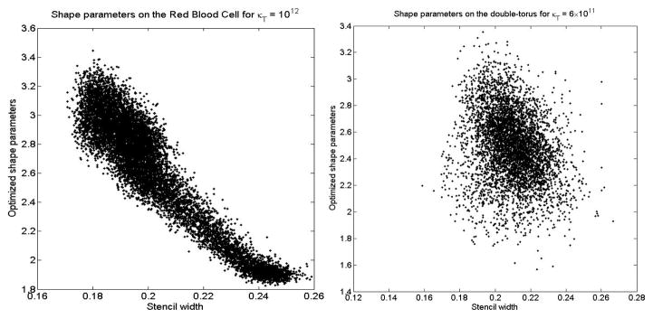
The figure on the left shows the computed shape parameters on the Red Blood Cell using N = 10000 MD nodes mapped to the Red Blood Cell (with κT = 1012) as a function of the stencil width. The figure on the right shows the computed shape parameters on the double-torus using using N = 5041 scattered nodes with κT = 6 × 10¹¹. In both cases, the stencil size is set to n = 31.
We note that it is possible to choose a single shape parameter in the above examples that is sufficiently large so that LX have all eigenvalues in the left half-plane (for example, ε = 3.4 for both the Red Blood Cell and the double-torus). However, this does not produce equally good results. The reason is that smaller shape parameters generally give better accuracy (cf. [28, 40]). Using the optimization procedure for selecting ε allows us to benefit from the accuracy afforded by smaller shape parameters where possible, as well as the stability afforded by larger shape parameters (when required by the irregularity of the node set). The trade-off in this procedure is that optimizing the shape parameter adds the cost of root-finding to the RBF-FD method. Additionally, fixing a target condition number across all stencils could mean that we end up choosing a lower condition number on some stencil than the condition number naturally dictated by the minimum width on that stencil. In this scenario, we are sacrificing some degree of local accuracy for the overall stability of the method. However, our tests did not reveal any impact of this on the convergence of the method.
While the shape parameter optimization procedure adds to the cost of our method, there are a few mitigating factors. First, we only solve the optimization problem to an absolute tolerance of 10−4; this proved sufficient for the purpose of stability and achieving the target condition number. Second (and more important), since the optimization is done on a per-stencil basis and the stencil computations themselves are easily parallelized, the overall optimization procedure itself is also embarrassingly parallel. These advantages are retained even if the surface sampled by the node set is evolving in time.
We conclude by noting that algorithms for the stable computation of RBF-FD matrices for all value of the shape parameters are available [28], but efforts to make these work for the case when the nodes are distributed on a lower dimensional surface embedded in ℝd is still needed. Though successful outcomes in this area would mean that we could use larger target condition numbers in our method, this does not necessarily imply the obsolescence of our optimization procedure. Given that current methods to stably compute RBF interpolants in planar domains are currently at least 5–10 times as costly as the standard RBF interpolation method, it is probable that new methods will have this drawback as well. In such a scenario, our shape parameter optimization procedure will likely allow for cost-efficient implementations of the RBF-FD method, allowing trade-offs between accuracy and computational cost.
6 Convergence studies
We now present the results illustrating the convergence of our method for the (forced) diffusion equation given in Equation (14) on some standard surfaces. We present experiments with two different optimization strategies. First, we present results for studies where we fix the condition number across all stencils for a given N, but allow the target condition number to grow with increasing N. Then, we present results for studies involving fixing the condition number for increasing N (equivalent to increasing the shape parameter for increasing N). In the latter case, we run into saturation errors [10] due to the employment of stationary interpolation. We use the Backward Difference Formula of Order 4 (BDF4) for all tests and set the time-step to Δt = 10−4, a time-step that allows the spatial errors to dominate the temporal error. We use BICGSTAB to solve the implicit system arising from the BDF4 discretization; we noticed that the solver needed at most three iterations per time-step to converge to a relative tolerance of 10−12. For convenience, we measure errors using the ℓ2 and ℓ∞ norms rather than approximations to the continuous versions of these norms on the test surfaces. The convergence of our method is a function of the fill distance hX, defined as the radius of the largest ball that is completely contained on the manifold which does not contain a node in X. For quasi-uniformly distributed nodes on our test surfaces, we expect that , where N is the total number of nodes on the surface. In the following subsections, we therefore examine convergence as a function of .
6.1 Convergence studies with increasing condition number
In this section, we present the results of numerical convergence studies where the uniform condition number across the RBF-FD matrices is allowed to grow as the number of points (N) on the surface increases. In the absence of the shape parameter optimization procedure, this would be equivalent to fixing the shape parameter while increasing N, the simplest approach to take with RBF interpolation.
First, we examine the convergence of our MOL formulation by approximating the diffusion equation on a sphere. Then, we examine the convergence of our method on simulating a forced diffusion equation on a torus. We present results for different stencil sizes n and examine convergence as the total number of nodes N increases.
Diffusion on the sphere
This test problem was presented in [29], and involves solving the heat equation on a unit sphere
. The exact solution to this problem is given as a series of spherical harmonics
, where θ and ϕ are longitude and latitude respectively, and Ylm is the degree l order m real spherical harmonic. Since the coefficients decay rapidly, the series is truncated after 30 terms. As in [29], we evolve the PDE until t = 0.5, using the exact solutions to boot-strap our BDF4 scheme. We test the RBF-FD method for n = 11, 17, and 31 for N = 642, 2562, 10242, and 40962 icosahedral points on the sphere [1], and plot the relative error in the numerical solutions. For all tests, we start with a target condition number of κT = 105 and allow it to grow with increasing N to κT = 1018. This effectively fixes the mean shape parameter on the surface as N grows. The results of this study are shown in Figure 4.
Fig. 4.

The figure on the left shows the ℓ2 error in the numerical solution to the diffusion equation on the sphere as a function of , while the figure on the right shows the ℓ∞ error. Both figures use a log-log scale, with colored lines indicating the errors in our method and dashed lines showing ideal p-order convergence for p = 2, 3, 4, 5. All errors were measured against the exact solution. The errors for n = 31 and N = 40962 were computed in quad-precision.
In addition to the errors, Figure 4 shows dashed lines corresponding to ideal p-order convergence, where p = 2, 3, 4, 5. It is clear that our method gives convergence between orders two and three for n = 11, close to order four for n = 17 and slightly higher than order five for n = 31, both in the ℓ2 and the ℓ∞ norms. Our method achieves similar results for smaller values of N than were used by the Closest Point method in [29], as is to be expected from a method that uses points only in the embedded space
. However, it is important to be cautious when comparing errors against the Closest Point method. The values of N given in the results in [29] are greater than the actual number of points used in that work to compute approximations to the Laplace-Beltrami operator. The values of N in that work correspond to all the points used in the embedding space ℝ3.
We note that the RBF-FD weights for n = 31 and N = 40962 were computed in quad-precision, though the simulations that used the weights were only run in double-precision. This is because our approach of allowing the condition number to grow with N leads to condition numbers of 1018 for very high N and n, which correspond to nearly-singular or singular matrices in double-precision. A possible way of remedying this is to start with a smaller target condition number for N = 642. Of course, this will lead to a higher error for each N, but can help offset the ill-conditioning for very large N and n. Later in this section, we will present an alternative way of ameliorating this issue.
Forced diffusion on a torus
This test is similar to the test presented in [23] involving randomly placed Gaussians on the sphere, except that this procedure is done on a torus. We consider the torus given by the implicit equation:
which can be parameterized using intrinsic coordinates φ and λ as follows:
| (17) |
where −π ≤ φ, λ ≤ π. The surface Laplacian of a scalar function f:
 → ℝ in this intrinsic coordinate system is given as
The manufactured solution to the diffusion equation (given by Equation (14) with
=
 ) is
) is
| (18) |
where a = 9, b = 3, and (φk, λk) are randomly chosen values in [−π, π]2. The solution is C∞(
) and a visualization at t = 0 is given in Figure 5 (left). While the solution and forcing function are all specified using intrinsic coordinates, the RBF-FD method uses only extrinsic (Cartesian coordinates) without requiring knowledge of the underlying intrinsic coordinate system. We compute the forcing function corresponding to Equation (18) analytically and evaluate it implicitly. We similarly compare errors in the numerical solution of the forced diffusion equation at time t = 0.2 for stencils of size n = 11, 17 and 31 nodes. The node sets we use for experiments on the torus are generated from a “staggered” grid in intrinsic variable space, and are determined as follows:
Fig. 5.
Forced diffusion on a torus. The figure on the left shows the intial condition for the forced diffusion problem on the torus given by Equation (17). The figure on the right shows a node set containing N = 5400 quasi-uniformly spaced nodes on the same torus.
Given m, choose m + 1 equally spaced angles on [−π, π] in φ and 3m + 1 equally spaced angles on [−π, π] in λ.
Disregard the values of φ and λ at π and take a direct product of the remaining points to obtain N = 3m2 points on [−π, π)2. Map these points to
using Equation (17) and call the set of nodes X1.Next, generate another set of N = 3m2 gridded points in [−π, π)2 from the previous set by offsetting the φ coordinate by π/m and the λ coordinate by π/(3m), so they lie at the midpoints of the previous gridded values. Map these to
and call the set of nodes X2.The final set of nodes is given by X = X1 ∪ X2.
In the experiments we use m = 10, 20, 30, 60, 80, corresponding to node sets of size N = 600, 2400, 5400, 21600, 38400. A plot of the nodes for N = 5400 is shown in Figure 5 (right). These points remain more or less uniformly spaced on the torus as N grows.
The results for the experiments are shown in Figure 6. Again, the figure shows dashed lines corresponding to ideal p-order convergence, where p = 2, 3, 4, 6. On this test, our method gives convergence of order two for n = 11, close to order four for n = 17 and between orders five and six for n = 31, both in the ℓ2 and the ℓ∞ norms. The convergence rates are comparable to the results seen for diffusion on the sphere. The results for n = 31 and N = 38400 were computed in quad-precision, for the same reasons as before.
Fig. 6.

The figure on the left shows the ℓ2 error in the numerical solution to the forced diffusion equation on the torus given by Equation (17) as a function of , while the figure on the right shows the ℓ∞ error. Both figures use a log-log scale, with colored lines indicating the errors in our method and dashed lines showing ideal p-order convergence for p = 2, 3, 4, 6. All errors were measured against the solution given by Equation (18). The errors for n = 31 and N = 38400 were computed in quad-precision.
6.2 Convergence studies with fixed condition number
In Section 6.1, we saw that allowing the target condition number to grow as N increases by fixing the mean shape parameter can give excellent results, but will eventually cause the RBF interpolation matrices to be ill-conditioned for large N and n.
In this section, we present an alternate approach. We choose to fix the target condition number at a particular (reasonably large) value for all values of N and n. As N increases, this has the effect of increasing the value of the average shape parameter. Our goal here is to understand the relationship between the magnitude of the target condition number and the value of n and N at which saturation errors can set in. This would also give us intuition on the connection between the target condition number and the order of convergence of our method.
With this in mind, we present the results of numerical convergence studies for two fixed condition numbers, κT = 1014 and κT = 1020, for increasing values of N and n. For κT = 1020, the RBF-FD weights on each patch were run in quad-precision using the Advanpix Multicomputing Toolbox. However, once the weights were obtained, they were converted back to double-precision and the simulations were carried out only in double-precision. We limit the presented results to those of the forced diffusion example on a torus from the previous section, but similar results were found for other examples. We again use a BDF4 method with Δt = 10−4, with the forcing term computed analytically and evaluated implicitly. The errors in the ℓ2 and ℓ∞ measured at t = 0.2 are shown in Figures 7–8.
Fig. 7.

The figure on the left shows the ℓ2 error in the numerical solution to the forced diffusion equation on the torus given by Equation (17) as a function of , while the figure on the right shows the ℓ∞ error. Both figures use a log-log scale, with colored lines indicating the errors in our method and dashed lines showing ideal p-order convergence for p = 2, 3, 4, 5. The target condition number was set to κT = 1014.
Fig. 8.

The figure on the left shows the ℓ2 error in the numerical solution to the forced diffusion equation on the torus given by Equation (17) as a function of , while the figure on the right shows the ℓ∞ error. Both figures use a log-log scale, with colored lines indicating the errors in our method and dashed lines showing ideal p-order convergence for p = 2, 3, 4, 6. The target condition number was set to κT = 1020 and all RBF-FD weights were computed in quad precision.
The results for κT = 1014 are shown in Figure 7, and those for κT = 1020 are shown in Figure 8. Figure 7 shows that fixing the target condition number at κT = 1014 produces no saturation errors in the ℓ2 or ℓ∞ norms for n = 11 or n = 17 in either norm. Indeed, κT = 1014 seems sufficient for methods up to order 4 for the values of N tested. However, for n = 31, we see saturation errors for N > 5400, again showing that larger target condition numbers are required for high-order RBF-FD methods.
Figure 8 shows that convergence of the solution for κT = 1020 and for n = 11 and 17 is similar to the case of κT = 1014 for the ℓ2 norm, with the errors for n = 11 being slightly lower for the ℓ∞ norm. For n = 31, we see that setting κT = 1020 actually results in an increased error in the solution over κT = 1014 in the case of N = 600, 2400 and 5400. However, as N is increased past 5400 nodes, the errors in the solution drop rapidly below those with κT = 1014 and the overall order of convergence for n = 31 appears to be between five and six. Since κT = 1020 results in smaller computed shape parameters than κT = 1014, these results imply that the errors can actually increase for a particular value of n and N as the shape parameter is reduced.
In order to better understand how the numerical solution to the forced diffusion equation on the torus behaves as a function of the target condition number κT, we fixed the stencil size at n = 31 and the node set at N = 38400 and computed relative errors in the solutions for κT = 108, 1012, …, 1024. The results are shown in Figure 9 from which we see the errors decreasing at a consistent rate as κT increases until around κT = 1020 at which point they level off, with a very slight increase as κT increases further. This shows that for a given value of N and n, there is an “optimal” target condition number beyond which it is pointless to further increase κT. An analogous way to view these results is in terms of the shape parameter. As κT increases, the overall magnitudes of the shape parameters across all stencils decrease and the radial kernels used to compute the stencil weights become increasingly flat. In this context, Figure 9 shows that the solutions become increasingly accurate for increasingly flat kernels, up to a point at which the accuracy cannot be improved, or actually degrades. This is entirely inline with other results in the RBF-FD literature involving a single shape parameter [40].
Fig. 9.

The figure shows the ℓ2 and ℓ∞ errors in the numerical solution to the forced diffusion equation on the torus given by Equation (17) as a function of the target condition number, κT. The figure uses a log-log scale. All RBF-FD weights for κT > 1014 were computed in quad-precision.
7 Application: Turing patterns
This section presents an application of our RBF-FD method to solving a two-species Turing system (two coupled reaction-diffusion equations) on different surfaces. We present two types of results, the first is for surfaces where parameterizations or implicit equations describing the surface are known, and the second where they are not. To facilitate comparison, we use the Turing system first described for the surface of the sphere in [37] and applied to more general surfaces in [23]. The system describes the interaction of an activator u and inhibitor v according to
| (19) |
| (20) |
If α = −γ, then (u, v) = (0, 0) is a unique equilibrium point of this system. Altering the diffusivity rates of u and v can lead to instabilities which manifest as pattern formations. The coupling parameter τ1 favors stripe formations, while τ2 favors spots. Stripe formations take much longer to attain “steady-state” than spot formations. In the following subsections, We use the Semi-implicit Backward Difference Formula of order 2 (SBDF2) as the time-stepping scheme, and set the time-step to Δt = 0.01 for all tests. Since the diffusion terms are handled implicitly, the RBF-FD matrix needs to be inverted every time-step. We accomplish this by pre-computing a sparse LU decomposition of the matrix, and using the triangular factors for forward and back solves every time-step. The values for all parameters for Equations (19) and (20), including final times for simulations, are presented in Table 1.
Table 1.
The above table shows the values of the parameters of Equations (19) and (20) used in the numerical experiments shown in Figures 10 and 11. In all cases, we set δu = 0.516δv.
| Surface/Pattern | δv | α | β | γ | τ1 | τ2 | Final time |
|---|---|---|---|---|---|---|---|
| RBC/spots | 4.5 × 10⁻³ | 0.899 | −0.91 | −0.899 | 0.02 | 0.2 | 800 |
| RBC/stripes | 2.1 × 10⁻³ | 0.899 | −0.91 | −0.899 | 3.5 | 0 | 6500 |
| Bumpy sphere/spots | 4.5 × 10⁻³ | 0.899 | −0.91 | −0.899 | 0.02 | 0.2 | 800 |
| Bumpy sphere/stripes | 2.1 × 10⁻³ | 0.899 | −0.91 | −0.899 | 3.5 | 0 | 7000 |
| Double-torus/spots | 2.1 × 10⁻³ | 0.899 | −0.91 | −0.899 | 0.02 | 0.2 | 700 |
| Double-torus/stripes | 8.87 × 10⁻⁴ | 0.899 | −0.91 | −0.899 | 3.5 | 0 | 6000 |
| Frog/spots | 2.87 × 10⁻⁴ | 0.899 | −0.91 | −0.899 | 0.02 | 0.2 | 600 |
| Bunny/stripes | 2.87 × 10⁻⁴ | 0.899 | −0.91 | −0.899 | 3.5 | 0 | 6000 |
7.1 Turing patterns on manifolds
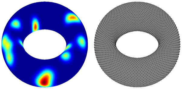
We first solve the Turing system on three surfaces: the Red Blood Cell (RBC) and the double-torus described earlier, and on the Bumpy Sphere detailed in [23]. RBCs are biconcave surfaces and can be represented parametrically, as described earlier. The Bumpy Sphere is a point set downloaded from an online repository, and equipped with point unit normals by parametric interpolation with the RBF parametric model presented in [32]. Also, since the downloaded model had N = 5256 vertices and we wished to demonstrate the viability of the RBF-FD method on far more vertices, we sampled our parametric model to generate N = 10000 vertices, and solve the Turing system on that point set. The first three rows of Table 2 list all the parameters used in the RBF-FD discretizations of Equations (19) and (20) on each of these three surfaces, and the last column of Table 1 lists the final times used for these simulations. The results of these simulations are shown in Figure 10. The spot and stripe patterns are qualitatively similar to those shown in [23].
Table 2.
The above table shows the values of the parameters used in the RBF-FD discretization of Equations (19) and (20) for the numerical experiments shown in Figures 10 and 11. In all cases, the time-step was set to Δt = 0.01.
| Surface | Number of nodes (N) | Stencil size (n) | Target Cond. No. (κT) |
|---|---|---|---|
| RBC | 10000 | 31 | 1012 |
| Bumpy sphere | 10000 | 31 | 1012 |
| Double-torus | 12100 | 31 | 1011 |
| Frog | 7458 | 31 | 1010 |
| Bunny | 11339 | 31 | 1010 |
Fig. 10.

Steady Turing spots and stripe patterns resulting from solving Equations (19) and (20) on the Red Blood Cell, the Bumpy Sphere model and the double-torus surfaces. In all plots, red corresponds to a high concentration of u and blue to a low concentration.
7.2 Turing patterns on more general surfaces
We now turn our attention to more general point sets: a Frog model (obtained from the AIM@SHAPE Shape Repository) and the Stanford Bunny model (obtained from the Stanford 3D Scanning Repository). Rather than as point clouds, these models are available in the form of meshes and approximate normal data. In contrast the previous two examples, it is not clear if the surfaces represented by these meshes can be analytically parametrized. To prepare these point sets for simulations, we first run the Poisson surface reconstruction algorithm [26] to generate a water-tight implicit surface that fits the point cloud. This algorithm requires both the point cloud and the approximate normals as input. Forming an implicit surface smoothes the approximate normal vectors input into the Poisson surface reconstruction, resulting in a more stable RBF-FD discretization. Having generated an implicit surface, we sample that with the Poisson disk sampling algorithm to generate a point cloud with the desired number of points. The other rationale for employing Poisson disk sampling is that while the Poisson surface reconstruction will fix any holes in the mesh, those former holes may not be sufficiently sampled. This pre-processing was performed entirely in MeshLab [6].
After this preprocessing, we run a Turing spot simulation on the Frog model, and a Turing stripe simulation on the Stanford Bunny. The last two rows of Table 2 list all the parameters used in the RBF-FD discretizations of Equations (19) and (20) on each of these surfaces, and the last column of Table 1 lists the final times used for these simulations. The results are shown in Figure 11. Before the color-mapping for aesthetics, the results are qualitatively similar to those shown in Figure 10.
Fig. 11.

The figure on the top right shows a Turing spot pattern on a Frog model. Green corresponds to a low concentration, and brown and black to higher concentrations. The figure on the bottom right shows a Turing stripe pattern on the Stanford Bunny model. Here, the lightest browns (almost white) correspond to low concentrations, and darker browns correspond to higher concentrations. Both the figures on the left show the point clouds used for the solution of the Turing system.
8 Discussion
In this paper, we introduced a new numerical method based on Radial Basis Function-generated Finite Differences (RBF-FD) for computing a discrete approximation to the Laplace-Beltrami operator on surfaces of codimension one embedded in ℝ3. The method uses scattered nodes on the surface, without requiring expansion into the embedding space. We improved on the method presented in [33], designing a stable numerical method that does not require stabilization with artificial viscosity (a feature of RBF-FD methods for convective flows). This development was facilitated by an algorithm to optimize the shape parameter for each interpolation patch on the surface. We demonstrated that this optimization procedure can compensate for irregularities in the sampling of the surface. We then presented error and convergence estimates for our method using two approaches: allowing the condition number to grow with the number of points on the surface, and fixing the condition number for an increasing number of points. We discussed the trade-offs inherent in each approach, and provided intuition as to the relationship between the condition number, shape parameter and the order of convergence of our method on the diffusion equation on a sphere and a torus. We presented an application of our method to simulating reaction-diffusion equations on surfaces; specifically, we demonstrated the solution of Turing PDEs on several interesting shapes, both parametrizable and more general.
While our method currently works for static objects, our goal is to apply RBF-FD to the solution of PDEs on evolving surfaces, with the evolution dictated by the interaction of a fluid with the object. It will be necessary to employ efficient and fast k-d tree implementations, including algorithms for dynamically updating and/or re-balancing the k-d tree as the point set evolves. The method will almost certainly need to be parallelized to be efficient.
One issue with our method is its ability to handle thin features on surfaces. Indeed, our method is not innately robust to such features. For RBF-FD to be robust on more general surfaces, it will be necessary to combine our method with an adaptive refinement code that detects thin features and samples sides of the feature sufficiently (the alternative would be to find an efficient way to measure distances along arbitrary surfaces).
A natural extension of this work would be to adapt the method to handle spatially-variable (possibly anisotropic) diffusion. While this extension is not conceptually difficult, the realization of this extension would make our method even more useful for biological applications, like the simulation of gels or viscoelastic materials on surfaces. We intend to address this in a follow-up study. Finally, while we have successfully applied RBF-FD to periodic surfaces, it would be interesting to apply the method to solving PDEs on surfaces with boundary conditions imposed on them. We intend to address this in a follow-up study as well.
Acknowledgments
We would like to acknowledge useful discussions concerning this work within the CLOT group at the University of Utah. The first, third and fourth authors acknowledge funding support under NIGMS grant R01-GM090203. The second author acknowledges funding support under NSF-DMS grant 1160379 and NSF-DMS grant 0934581.
Contributor Information
Varun Shankar, Email: shankar@cs.utah.edu, School of Computing, University of Utah, Salt Lake City, UT 84112.
Grady B. Wright, Email: gradywright@boisestate.edu, Department of Mathematics, Boise State University, Boise, ID 83725-1555
Robert M. Kirby, Email: kirby@sci.utah.edu, School of Computing, University of Utah, Salt Lake City, UT 84112
Aaron L. Fogelson, Email: fogelson@math.utah.edu, Department of Mathematics, University of Utah, Salt Lake City, UT 84112
References
- 1.Baumgardner JR, Frederickson PO. Icosahedral discretization of the Two-Sphere. SIAM Journal on Numerical Analysis. 1985;22(6):1107–1115. doi: 10.1137/0722066. URL http://dx.doi.org/10.1137/0722066. [DOI] [Google Scholar]
- 2.Bayona V, Moscoso M, Carretero M, Kindelan M. Rbf-fd formulas and convergence properties. Journal of Computational Physics. 2010;229(22):8281–8295. [Google Scholar]
- 3.Calhoun D, Helzel C. A finite volume method for solving parabolic equations on logically cartesian curved surface meshes. SIAM Journal on Scientific Computing. 2010;31(6):4066–4099. doi: 10.1137/08073322X. URL http://epubs.siam.org/doi/abs/10.1137/08073322X. [DOI] [Google Scholar]
- 4.Cecil T, Qian J, Osher S. Numerical methods for high dimensional Hamilton-Jacobi equations using radial basis functions. J Comput Phys. 2004;196:327–347. [Google Scholar]
- 5.Chandhini G, Sanyasiraju Y. Local RBF-FD solutions for steady convection–diffusion problems. International Journal for Numerical Methods in Engineering. 2007;72(3):352–378. [Google Scholar]
- 6.Cignoni P, Corsini M, Ranzuglia G. Meshlab: an open-source 3d mesh processing system. ERCIM News. 2008;(73):45–46. URL http://vcg.isti.cnr.it/Publications/2008/CCR08.
- 7.Davydov O, Oanh D. Adaptive meshless centres and rbf stencils for poisson equation. Journal of Computational Physics. 2011;230(2):287–304. [Google Scholar]
- 8.Driscoll T, Fornberg B. Interpolation in the limit of increasingly flat radial basis functions. Computers & Mathematics with Applications. 2002;43(3):413–422. [Google Scholar]
- 9.Dziuk G, Elliott CM. Finite elements on evolving surfaces. IMA Journal of Numerical Analysis. 2007;27(2):262–292. doi: 10.1093/imanum/drl023. URL http://imajna.oxfordjournals.org/content/27/2/262.abstract. [DOI] [Google Scholar]
- 10.Fasshauer GE. Interdisciplinary Mathematical Sciences. Vol. 6. World Scientific Publishers; Singapore: 2007. Meshfree Approximation Methods with MATLAB. [Google Scholar]
- 11.Fasshauer GE, McCourt MJ. Stable evaluation of Gaussian radial basis function interpolants. SIAM Journal on Scientific Computing. 2012;34:A737–A762. [Google Scholar]
- 12.Flyer N, Lehto E, Blaise S, Wright G, St-Cyr A. A guide to RBF-generated finite differences for nonlinear transport: shallow water simulations on a sphere. Journal of Computational Physics. 2012;231:4078–4095. [Google Scholar]
- 13.Flyer N, Wright GB. Transport schemes on a sphere using radial basis functions. J Comp Phys. 2007;226:1059–1084. [Google Scholar]
- 14.Flyer N, Wright GB. A radial basis function method for the shallow water equations on a sphere. Proc Roy Soc A. 2009;465:1949–1976. [Google Scholar]
- 15.Fornberg B, Driscoll TA, Wright G, Charles R. Observations on the behavior of radial basis functions near boundaries. Comput Math Appl. 2002;43:473–490. [Google Scholar]
- 16.Fornberg B, Larsson E, Flyer N. Stable computations with Gaussian radial basis functions. SIAM Journal on Scientific Computing. 2011;33(2):869–892. [Google Scholar]
- 17.Fornberg B, Lehto E. Stabilization of RBF-generated finite difference methods for convective PDEs. Journal of Computational Physics. 2011;230:2270–2285. [Google Scholar]
- 18.Fornberg B, Lehto E, Powell C. Stable calculation of Gaussian-based RBF-FD stencils. Comp Math Applic. 2013;65:627–637. [Google Scholar]
- 19.Fornberg B, Piret C. A stable algorithm for flat radial basis functions on a sphere. SIAM Journal on Scientific Computing. 2007;30:60–80. [Google Scholar]
- 20.Fornberg B, Wright G. Stable computation of multiquadric interpolants for all values of the shape parameter. Comput Math Appl. 2004;48:853–867. [Google Scholar]
- 21.Fornberg B, Zuev J. The Runge phenomenon and spatially variable shape parameters in RBF interpolation. Comput Math Appl. 2007;54:379–398. [Google Scholar]
- 22.Fuselier E, Wright G. Scattered data interpolation on embedded submanifolds with restricted positive definite kernels: Sobolev error estimates. SIAM Journal on Numerical Analysis. 2012;50(3):1753–1776. doi: 10.1137/110821846. URL http://epubs.siam.org/doi/abs/10.1137/110821846. [DOI] [Google Scholar]
- 23.Fuselier EJ, Wright GB. A high-order kernel method for diffusion and reaction-diffusion equations on surfaces. Journal of Scientific Computing. 2013:1–31. doi: 10.1007/s10915-013-9688-x. URL http://dx.doi.org/10.1007/s10915-013-9688-x. [DOI] [PMC free article] [PubMed]
- 24.George A, Liu JW. Prentice Hall Professional Technical Reference. 1981. Computer Solution of Large Sparse Positive Definite. [Google Scholar]
- 25.Gia QTL. Approximation of parabolic pdes on spheres using spherical basis functions. Adv Comput Math. 2005;22:377–397. [Google Scholar]
- 26.Kazhdan M, Bolitho M, Hoppe H. Poisson surface reconstruction. Proceedings of the Fourth Eurographics Symposium on Geometry Processing, SGP ‘06; Aire-la-Ville, Switzerland, Switzerland: Eurographics Association; 2006. pp. 61–70. URL http://dl.acm.org/citation.cfm?id=1281957.1281965. [Google Scholar]
- 27.Larsson E, Fornberg B. Theoretical and computational aspects of multivariate interpolation with increasingly flat radial basis functions. Comput Math Appl. 2005;49:103–130. [Google Scholar]
- 28.Larsson E, Lehto E, Heryudono A, Fornberg B. Stable computation of differentiation matrices and scattered node stencils based on gaussian radial basis functions. SIAM Journal on Scientific Computing. 2013;35(4):A2096–A2119. doi: 10.1137/120899108. [DOI] [Google Scholar]
- 29.Macdonald C, Ruuth S. The implicit closest point method for the numerical solution of partial differential equations on surfaces. SIAM Journal on Scientific Computing. 2010;31(6):4330–4350. doi: 10.1137/080740003. URL http://epubs.siam.org/doi/abs/10.1137/080740003. [DOI] [Google Scholar]
- 30.Piret C. The orthogonal gradients method: A radial basis functions method for solving partial differential equations on arbitrary surfaces. J Comput Phys. 2012;231(20):4662–4675. [Google Scholar]
- 31.Schaback R. Multivariate interpolation by polynomials and radial basis functions. Constr Approx. 2005;21:293–317. [Google Scholar]
- 32.Shankar V, Wright GB, Fogelson AL, Kirby RM. A study of different modeling choices for simulating platelets within the immersed boundary method. Applied Numerical Mathematics. 2013;63(0):58–77. doi: 10.1016/j.apnum.2012.09.006. URL http://www.sciencedirect.com/science/article/pii/S0168927412001663. [DOI] [PMC free article] [PubMed] [Google Scholar]
- 33.Shankar V, Wright GB, Fogelson AL, Kirby RM. A radial basis function (rbf) finite difference method for the simulation of reactiondiffusion equations on stationary platelets within the augmented forcing method. International Journal for Numerical Methods in Fluids. 2014 doi: 10.1002/3d.3880. pp. n/a–n/a. URL http://dx.doi.org/10.1002/fld.3880. [DOI]
- 34.Shu C, Ding H, Yeo K. Local radial basis function-based differential quadrature method and its application to solve two-dimensional incompressible navier–stokes equations. Computer Methods in Applied Mechanics and Engineering. 2003;192(7):941–954. [Google Scholar]
- 35.Stevens D, Power H, Lees M, Morvan H. The use of PDE centers in the local RBF Hermitean method for 3D convective-diffusion problems. J Comput Phys. 2009;228:4606–4624. [Google Scholar]
- 36.Tolstykh A, Shirobokov D. On using radial basis functions in a finite difference mode with applications to elasticity problems. Computational Mechanics. 2003;33(1):68–79. [Google Scholar]
- 37.Varea C, Aragon J, Barrio R. Turing patterns on a sphere. Phys Rev E. 1999;60:4588–4592. doi: 10.1103/physreve.60.4588. [DOI] [PubMed] [Google Scholar]
- 38.Wendland H. Cambridge Monographs on Applied and Computational Mathematics. Vol. 17. Cambridge University Press; Cambridge: 2005. Scattered data approximation. [Google Scholar]
- 39.Womersley RS, Sloan IH. Interpolation and cubature on the sphere. Website. 2007 http://web.maths.unsw.edu.au/~rsw/Sphere/
- 40.Wright GB, Fornberg B. Scattered node compact finite difference-type formulas generated from radial basis functions. Journal of Computational Physics. 2006;212(1):99–123. doi: 10.1016/j.jcp.2005.05.030. URL http://www.sciencedirect.com/science/article/pii/S0021999105003116. [DOI] [Google Scholar]