Computational analysis of the effectiveness of blood flushing with saline injection from an intravascular diagnostic catheter

SUMMARY

Optical techniques including fluorescence lifetime spectroscopy have demonstrated potential as a tool for study and diagnosis of arterial vessel pathologies. However, their application in the intravascular diagnostic procedures has been hampered by the presence of blood hemoglobin that affects the light delivery to and the collection from the vessel wall. We report a computational fluid dynamics model that allows for the optimization of blood flushing parameters in a manner that minimizes the amount of saline needed to clear the optical field of view and reduces any adverse effects caused by the external saline jet. A 3D turbulence (k−ω) model was employed for Eulerian–Eulerian two-phase flow to simulate the flow inside and around a side-viewing fiber-optic catheter. Current analysis demonstrates the effects of various parameters including infusion and blood flow rates, vessel diameters, and pulsatile nature of blood flow on the flow structure around the catheter tip. The results from this study can be utilized in determining the optimal flushing rate for given vessel diameter, blood flow rate, and maximum wall shear stress that the vessel wall can sustain and subsequently in optimizing the design parameters of optical-based intravascular catheters.

1. INTRODUCTION

Optical-based intravascular diagnostic techniques are emerging as promising tools for assessment of atherosclerotic plaque vulnerability and other cardiovascular pathologies. Examples of such techniques include optical coherence tomography [1, 2], laser speckle imaging [3], photoacoustic imaging [4–6], and a range of spectroscopic methods (Raman, near-infrared (NIR), diffuse reflectance NIR, and fluorescence spectroscopy) [7–13]. One problem hampering the broader clinical intravascular validation and application of several optical methods is the presence of blood in the optical pathway [14, 15]. In particular, this is the case for emerging fluorescence spectroscopy or imaging techniques that have the potential for intravascular characterization of atherosclerotic composition. For example, the presence of lipids components and inflammation in the intima fibrotic cap play an important role in plaque instability and rupture [16–18]. The blood hemoglobin attenuates the optical signal and diminishes the sensitivity of detection (signal-to-noise ratio). Techniques such as saline bolus injection or balloon occlusion are typically used to temporarily remove the blood during such interventions. However, such techniques are not feasible for continuous optical scanning of long arterial segments. Balloon occlusion may also result in damage to the vessel wall.

Moreover, intravascular injection of fluids via catheters is not only used for saline injection but also for intra-arterial infusion of contrast agents or drugs for localized treatment of arterial pathologies while reducing the risks of the side effects of systemic delivery of such substances. Typically, the injection of substance is accomplished through separate holes (ports) located along the surface of the tip, generally distant from one another, to avoid recirculation effects. However, damage of the vessel wall can occur if the injection rate is not controlled properly, depending on the geometrical configuration of catheter tip, the type of vessel, and the physical and mechanical properties of the vessel wall and atherosclerotic plaque [19]. Possible consequences of the high flow rate is vessel wall perforation or plaque disrupture caused by the jet exiting the catheter tip [20–22]. Many of these complications due to high flow rate are linked to the complexity of the flow field [23–25]. It is, therefore, important to study the flow pattern and its effects on wall shear stress (WSS) around the catheter tip.

Numerical and experimental investigations by various researchers in the related area in the recent years can provide valuable insight into the complex flow structure for incompressible two-phase cross flow [26–30]. Foust et al. [24] studied the structure of the jet from a generic catheter tip with a side hole with high-image density particle image velocimetry. Numerical and experimental studies by Weber et al. [31] provided flow structures and effect on WSS for peripheral IV catheters with multiple side holes with constant blood for 3, 5, and 7 mm diameter blood vessel. Varghese et al. [32] reported a detailed numerical study of pulsatile turbulent single-phase flow in stenotic vessel using four different turbulence models: k – ∊, renormalization group theory k− ∊ [33], standard k – ω, and k − ω with low Reynolds number correction. They found k − ω turbulence model with low Reynolds number correction to produce better results as compared with the other models. However, all these investigations have been limited to specific types of catheter tip configuration where the catheter is placed concentrically with the blood vessel and the blood flow rate is assumed to be constant. Also, none of the studies have focused on the clearance of blood in the pathway of the jet exiting from the catheter tip. Ghata et al. [34] reported numerical investigation of the catheter flow and its effects on WSS, wall pressure, and the distribution of the blood cells for the exact same catheter configuration that is similar with that considered in this study. However, the authors employed the multiphase mixture model with a k −∊ turbulence model in their study. The current study employs both Eulerian–Eulerian multiphase and mixture models and a k − ω turbulence model with low Reynolds number correction. In the mixture model, the continuity and momentum equations for the mixture, the volume fraction equation, and the relative velocities of the secondary phases are solved, and the phase interaction is modeled through an algebraic relationship, whereas the Eulerian model solves the conservation equations for each phase separately. Therefore, one needs to solve fewer equations in the mixture model as than in the Eulerian model. The mixture model thus requires less computational effort, although the Eulerian model gives better accuracy [35].

This study analyzes the flow around a special type of catheter that is equipped with a fiber-optic probe for light delivery and collection to/from the vessel wall. The objectives of this study are to see the feasibility of employing the mixture model and qualitatively compare the results for the possible range of parameters that include (a) blood flow rates arteries of equal diameter, in order to account for systolic and diastolic conditions; (b) vessels with two different diameters but the same blood flow rate and injection rate, to determine the effect on stenotic vessels; (c) two different injection rates for the same blood flow rate and vessel diameter to determine the effect of the jet injection rate and (d) pulsatile blood flow.

2. METHOD

A number of studies [36–41] have shown that blood being a suspension of corpuscles behaves like a non-Newtonian fluid at low shear rate less than 20/s. Theoretical study by Haynes [42] and experimental observation by Cokelet [39] show that blood can be treated as single-phase homogenous viscous fluid when the diameter of vessels is greater than 1 mm. Also, Haynes [42] concludes from his study that the Fahraeus–Lindqvist effect occurs in blood vessels less than 0.4 mm in diameter. Jung et al. [43] performed a numerical investigation of a pulsatile blood flow in a coronary artery, including a detailed study of multiphase effects in large-curved blood vessels (D = 4.37 mm). Their study shows a very small effect of multiphase behavior of blood on WSS at the inner region of the curvature, whereas the single-phase model overpredicts the maximum WSS at the outer region by about 20%. The current study focuses on flow in a straight segment of a large blood vessel (diameter ≥3 mm). Therefore, curvature effects can be neglected in our study. For vessel diameter much larger than 0.4 mm, the Fahraeus–Lindqvist effect can be neglected, and blood can be assumed to be Newtonian [44, 45].

Cho et al. [46] performed a numerical study of the effects of blood vessel properties on blood flow characteristics in stenosed arteries using fluid-structure interaction. Their studies show that the rigid vessel assumption underpredicts WSS by about 20%. The current study, however, focuses on nondeformable vessels.

A finite volume method-based commercial code ANSYS FLUENT v12.1 was used for the numerical simulations. The computational domain consisting of the catheter and the blood vessel is shown in Figure 1(a). A straight arterial segment of 96-cm length with a diameter of either 6 or 3 mm is considered for the simulations. The computational domain was discretized into an unstructured tetrahedral mesh using the ANSYS ICEM CFD v12.1 mesh generation tool. Figure 1(b) shows a part of the mesh generated on the catheter and blood vessel.

Figure 1.

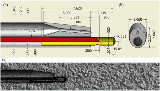
2D schematic view of the catheter: (a) top view and (b) side view (all dimensions are in mm) and (c) computational tetrahedral mesh at the midplane.

A second order upwind scheme was used for solution of the momentum equations, volume fraction, turbulent kinetic energy, and dissipation rate. A coupled algorithm was used to resolve the coupling of pressure and velocity. To accelerate the convergence, the relaxation factors for both momentum and pressure were taken as 0.5 and under-relaxation factors for volume fraction, turbulent kinetic energy, and dissipation rate were taken as 0.4, 0.8, and 0.8 respectively. The transient formulation was performed using second order implicit method with time step of 0.001 s. The uniform blood flow cases were simulated for 3 s, and the pulsatile case with period (T) of 0.75 s was computed for four cycles (3.0 s).

The density and viscosity of blood are taken as 1170 kg/m³ and 0.0035 Pa-s respectively and those of the saline solution are 1500 kg/m³ and 0.018 Pa-s, respectively. The inlet parameters for the five cases that were studied are listed in Table I. For the pulsatile case, the mean blood flow rate $({\dot{Q}}_0)$ is taken as 6.915 ml/s, and the average difference between the maximum and minimum blood flow rate $({\dot{Q}}_m)$ is 2.305 ml/s.

Table I.

Flow parameters used simulations.

Case	d (mm)	Aeff (mm2)	Ac (mm2)	${\dot{Q}}_b$ (ml/s)	${\dot{Q}}_s$ (ml/s)
1	6	24.27	0.5893	9.22	1.25
2	6	24.27	0.5893	4.61	1.25
3	3	3.077	0.5893	9.22	1.25
4	3	3.077	0.5893	9.22	0.625
5	6	24.27	0.5893	9.22	1.25

2.1. Eulerian multiphase flow model

The local transport equations governing the flow of each distinct phase are based on three key principles: conservation of mass, momentum, and energy. Another equation comes from the fact that the volume of a phase can not be occupied by another phase but they together occupy the entire domain of interest. So, the sum of the volume fractions of all the phases is equal to one. We end up dropping the energy equation based on the assumption that there is no temperature gradient present in the system. Also, all the phases are assumed to be incompressible in our current study. It follows that the equations for incompressible flow of N phases or components are given by the conservation of mass and momentum of each phase.

The mass transfer equation for each phase α is given by

$$\frac{\partial {\rho }_{\alpha }{\varphi }_{\alpha }}{\partial t}+\nabla .({\rho }_{\alpha }{\varphi }_{\alpha }{\overrightarrow{v}}_{\alpha })=0$$ (1)

where ρ_α is the density, ϕ_α is the volume fraction/concentration, ${\overrightarrow{v}}_{\alpha }$ is the velocity of phase α, and t is the time. The previous equation is based on the assumption that the source term is zero for all phases meaning that there is no generation or removal of any phase from the system other than the transport because of convection and diffusion.

Momentum conservation for each phase α is given by

$$\frac{\partial }{\partial t}({\rho }_{\alpha }{\varphi }_{\alpha }{\overrightarrow{v}}_{\alpha })+\nabla .({\rho }_{\alpha }{\varphi }_{\alpha }{\overrightarrow{v}}_{\alpha }{\overrightarrow{v}}_{\alpha })=-{\varphi }_{\alpha }\nabla P+\nabla .({\varphi }_{\alpha }\overline{\overline{\tau }})+{\displaystyle \sum _{p=1}^N{\overrightarrow{R}}_{\beta \alpha }}$$ (2)

where P is the pressure, R_βα accounts for the interfacial forces between phases α and β is given by Eq. (5). The stress tensor, $\overline{\overline{\tau }}$ in Eq. (2) is given by

$$\overline{\overline{\tau }}={\mu }_{\alpha }(\nabla {\overrightarrow{v}}_{\alpha }+\nabla {\overrightarrow{v}}_{\alpha }^T)+\left({\lambda }_{\alpha }-\frac{2}{3}{\mu }_{\alpha }\right)\nabla .{\overrightarrow{v}}_{\alpha }\overline{\overline{I}}$$ (3)

where μ_α and λ_α are the shear and bulk viscosities of phase α.

The species conservation is given by

$${\displaystyle \sum _{\alpha =1}^N{\varphi }_{\alpha }=1}$$ (4)

This indicates that summation of the volume fraction of all the phases is 1.0.

The interfacial force, ${\overrightarrow{R}}_{\beta \alpha }$, in Eq. (2) that acts on phase α because of the presence of phase β is given by

$${\overrightarrow{R}}_{\beta \alpha }=K_{\beta \alpha }({\overrightarrow{v}}_{\alpha }-{\overrightarrow{v}}_{\beta })$$ (5)

where K_αβ is the interphase momentum exchange coefficient and for liquid–liquid mixtures, this can be expressed as [35]

$$K_{\alpha \beta }=\frac{{\varphi }_{\alpha }{\varphi }_{\beta }{\rho }_{\alpha }f}{{\tau }_{\alpha }}$$ (6)

For fluid–fluid flows, each secondary phase is assumed to form droplets or bubbles [35]. The particulate relaxation time (τ_α) is defined as

$${\tau }_{\alpha }=\frac{{\rho }_{\alpha }{d}_{\alpha }^2}{18{\mu }_{\alpha }}$$ (7)

where d_α is the diameter of the bubbles or droplets of phase α. The drag function (f) in Eq. (6) is given by [35]

$$f=\frac{C_{D}Re}{24}$$ (8)

where the drag coefficient (C_D) is estimated using the following empirical relation

$$C_D=\{\begin{array}{ll}\frac{24}{\mathit{Re}}(1+0.15{\mathit{Re}}^{0.687})\hfill & \text{if}\mathit{Re}\le 1000\hfill \\ 0.44\hfill & \text{otherwise}\hfill \end{array}$$

The relative Reynolds number (Re) for the primary phase α and the secondary phase β is obtained from\

$$\mathit{Re}=\frac{{\rho }_{\alpha }|{\overrightarrow{v}}_{\alpha }-{\overrightarrow{v}}_{\beta }|d_p}{{\mu }_{\alpha }}$$ (9)

2.2. Turbulence modeling

In deriving Reynolds-averaged Navier–Stokes equations, the solution variables in Eqs. (1)–(2) are decomposed into two parts: the mean space (ensemble averaged or time averaged) and the fluctuating components. For example, the instantaneous velocity vector can be written as

$$\overrightarrow{v}=\overrightarrow{\overline{v}}+\overrightarrow{\acute{v}}$$ (10)

where $\overrightarrow{\overline{v}}$ and $\overrightarrow{\acute{v}}$ are the mean and fluctuating velocity vectors, respectively. Similarly, scalar variables like pressure are expressed as

$$\phi =\overline{\phi }+\overrightarrow{\acute{\phi }}$$ (11)

After substituting the expression of the variables into the continuity and momentum equations and taking time or ensemble average (dropping the overbar for conveniences), the Eqs. (1) and (2) reduce to

$$\frac{\partial }{\partial t}({\rho }_{\alpha }{\varphi }_{\alpha })+\nabla .({\rho }_{\alpha }{\varphi }_{\alpha }{\overrightarrow{v}}_{\alpha })=0$$ (12)

$$\begin{array}{l}\frac{\partial }{\partial t}({\rho }_{\alpha }{\varphi }_{\alpha }{\overrightarrow{v}}_{\alpha })+\nabla .({\rho }_{\alpha }{\varphi }_{\alpha }{\overrightarrow{v}}_{\alpha }{\overrightarrow{v}}_{\alpha })=-{\varphi }_{\alpha }\nabla P\\ +\nabla .\left[{\varphi }_{\alpha }\right({\overline{\overline{\tau }}}_{\alpha }+{\overline{\overline{\tau }}}_{\alpha }^t\left)\right]+{\displaystyle \sum _{\beta =1}^N{\overrightarrow{R}}_{\beta \alpha }}\end{array}$$ (13)

where the viscous stress tensor $({\overline{\overline{\tau }}}_{\alpha })$ is given by Eq. (3). Reynolds shear stress term $({\overline{\overline{\tau }}}_{\alpha }^t)$ where the viscous stress tensor

$${\overline{\overline{\tau }}}_{\alpha }^t=-{\rho }_{\alpha }\langle {\acute{\overrightarrow{v}}}_{\alpha }{\acute{\overrightarrow{v}}}_{\alpha }\rangle$$ (14)

Equations (12) and (13) are called Reynolds-averaged Navier–Stokes equations. Various turbulence modeling schemes like K−∊, K − ω can be used to calculate Reynolds stress tensor ${\overline{\overline{\tau }}}_{\alpha }^t$. K – ω turbulence modeling with low Reynolds number correction has been employed for the simulation of Reynolds shear stress [35]:

$$\begin{array}{l}-{\rho }_{\alpha }\langle {\acute{\overrightarrow{v}}}_{\alpha }{\acute{\overrightarrow{v}}}_{\alpha }\rangle ={\mu }_{\alpha }^t\left(\frac{\partial v_{\alpha i}}{\partial x_j}+\frac{\partial v_{\alpha j}}{\partial x_i}\right)\\ -\frac{2}{3}\left({\rho }_{\alpha }{k}_{\alpha }+{\mu }_{\alpha }^t\frac{\partial v_{\alpha l}}{\partial x_l}\right){\delta }_{\mathit{ij}}\end{array}$$ (15)

where the turbulent viscosity, ${{\mu }_{\alpha }}^t$ is computed by

$${{\mu }_{\alpha }}^t=\frac{{\rho }_{\alpha }{k}_{\alpha }}{{\omega }_{\alpha }}$$ (16)

The turbulence kinetic energy, k_α, and the specific dissipation rate, ω_α, for each phase α are calculated from the following transport equations

$$\frac{\partial }{\partial t}({\rho }_{\alpha }{k}_{\alpha })+\nabla .({\rho }_{\alpha }{k}_{\alpha })=\nabla .({\mathrm{\Gamma }}_{k\alpha }\nabla k_{\alpha })$$ (17)

$$\frac{\partial }{\partial t}({\rho }_{\alpha }{\omega }_{\alpha })+\nabla .({\rho }_{\alpha }{\omega }_{\alpha })=\nabla .({\mathrm{\Gamma }}_{\omega \alpha }\nabla {\omega }_{\alpha })$$ (18)

2.3. Mixture model

In the previous section, we have discussed Eulerian multiphase model where the conservation equations for each of the phases are solved separately.

The mass conservation is given by

$$\frac{\partial (\rho )}{\partial t}+\nabla .(\rho \overrightarrow{v})=0$$ (19)

where $\overrightarrow{v}$ is the mass-averaged velocity, given by

$$\overrightarrow{v}=\frac{{\displaystyle \sum _{\alpha }{\varphi }_{\alpha }{\rho }_{\alpha }{\overrightarrow{v}}_{\alpha }}}{\rho }$$ (20)

α = Blood, Saline and the mixture density ρ is given by

$$\rho ={\displaystyle \sum _{\alpha }{\varphi }_{\alpha }{\rho }_{\alpha }}$$ (21)

The momentum conservation for the mixture is given by

$$\frac{\partial (\rho \overrightarrow{v})}{\partial t}+\nabla .(\rho \overrightarrow{v}\overrightarrow{v})=-\nabla P+\nabla .\left[\mu (\nabla \overrightarrow{v}+\nabla {\overrightarrow{v}}^T)\right]+\rho \overrightarrow{g}+\nabla .\left({\displaystyle \sum _{\alpha }{\varphi }_{\alpha }{\rho }_{\alpha }{\overrightarrow{v}}_{\mathit{dr},\alpha }{\overrightarrow{v}}_{\mathit{dr},\alpha }}\right)$$ (22)

where P is the mixture pressure. The mixture viscosity μ and drift velocity ${\overrightarrow{v}}_{\mathit{dr},\alpha }$ of phase α are given as follows:

$$\mu ={\displaystyle \sum _{\alpha }{\varphi }_{\alpha }{\mu }_{\alpha }}$$ (23)

$${\overrightarrow{v}}_{\mathit{dr},\alpha }={\overrightarrow{v}}_{\alpha m}-{\displaystyle \sum _{\beta }{Y}_{\beta }{\overrightarrow{v}}_{m\beta }}$$ (24)

where the subscript m indicates mixture and the slip or relative velocity ${\overrightarrow{v}}_{\alpha ,\beta }$ is defined as the velocity of the secondary phase α relative to primary phase β:

$${\overrightarrow{v}}_{\alpha \beta }={\overrightarrow{v}}_{\alpha }-{\overrightarrow{v}}_{\beta }$$ (25)

and the mass fraction Y_β of phase β is defined as

$$Y_{\beta }=\frac{{\varphi }_{\beta }{\rho }_{\beta }}{\rho }$$ (26)

In turbulent flows, the relative velocity is given by

$${\overrightarrow{v}}_{\alpha \beta }=\frac{({\rho }_{\alpha }-\rho )d_{\alpha }^2}{18{\mu }_{\beta }{f}_{\mathit{\text{drag}}}}\overrightarrow{a}-\frac{{\eta }_t}{{\sigma }_t}\left(\frac{\nabla {\varphi }_{\alpha }}{{\varphi }_{\alpha }}-\frac{\nabla {\varphi }_{\beta }}{{\varphi }_{\beta }}\right)$$ (27)

where σ_t is Schmidt number and is set to 0.75, and for k − ∊ turbulent model, the diffusion coefficient η_t is given by [47, 48]

$${\eta }_t=C_{\mu }\frac{k^2}{\mathit{∊}}\left(\frac{{\nu }_{\nu }}{1+{\nu }_{\nu }}\right){(1+C_{\beta }{\zeta }_{\nu }^2)}^{-\frac{1}{2}}$$ (28)

$${\zeta }_{\nu }=\frac{\left|{\overrightarrow{v}}_{\alpha \beta }\right|}{\sqrt{\frac{2k}{3}}}$$ (29)

where C_β = 0:85 and f_drag is given by [49]:

$$f_{\mathit{\text{drag}}}=1+0.15R{e}^{0.687}Re\le 1000$$ (30)

$$=0.0183\mathit{Re}\mathit{Re}>1000$$ (31)

and acceleration $\overrightarrow{a}$ is given as

$$\overrightarrow{a}=\overrightarrow{g}-(\overrightarrow{v}.\nabla )\overrightarrow{v}-\frac{\partial \overrightarrow{v}}{\partial t}$$ (32)

2.4. Boundary conditions

At the inlet to the blood vessel

$$\text{Normal blood}\text{velocity}:\overrightarrow{v}.\overrightarrow{n}=\frac{{\dot{Q}}_b}{A_{\mathit{eff}}}$$ (33)

$$\text{Saline concentration}:{\varphi }_s-0$$ (34)

where A_eff is the effective cross sectional area of the blood vessel at the inlet as a result of the catheter insertion. ${\dot{Q}}_b$ is the blood flow rate that is assumed to be constant for cases (1 – −4) and a periodic function of time for pulsatile case 5. For pulsatile flow, ${\dot{Q}}_b$ is assumed to vary between the maximum and minimum flow rates in a sinusoidal function [32].

$${\dot{Q}}_b(t)={\dot{Q}}_0-{\dot{Q}}_m\mathit{cos}\left(\frac{2\mathrm{\Pi }t}{T}\right)$$ (35)

${\dot{Q}}_0$ is the mean blood flow rate, and ${\dot{Q}}_m$ is taken as half of the difference between maximum $({\dot{Q}}_{\mathit{max}})$ and minimum $({\dot{Q}}_{\mathit{min}})$ blood flow rate. T is the time period of the pulsatile flow.

Note that although this model is not a quantitatively accurate representation of pulsatile blood flow, it does allow qualitative examination of its influence on WSS.

At the inlet to the catheter

$$\text{Normal blood velocity}:\overrightarrow{v}.\overrightarrow{n}=\frac{{\dot{Q}}_s}{A_c}$$ (36)

$$\text{Saline concentration}:{\varphi }_s=1.0$$ (37)

where A_c is the area injection of catheter section at the inlet.

At the vessel and catheter walls, no-slip boundary condition is imposed:

$$\overrightarrow{v}=\overrightarrow{0}$$ (38)

At the outlet, prescribed velocity or pressure outlet boundary conditions are typically employed. However, a velocity or pressure outlet condition is inappropriate when modeling wave-propagation phenomena in human arteries because obtaining time-varying velocity or pressure at the outlet is impractical. Vignon-Clementel et al. [50] has applied the outflow boundary condition for 3D simulations of nonperiodic blood flow in deformable arteries. The outflow boundary condition has been also employed in other studies [51–54] in arterial hemodynamics simulations. We, therefore, impose the following outflow boundary condition at the vessel outlet.

$$\frac{d}{\mathit{dt}}{\displaystyle \underset{\mathrm{\Omega }}{\int }{\rho }_{\alpha }d\mathrm{\Omega }}+{\displaystyle \underset{\mathrm{\Gamma }}{\int }{\rho }_{\alpha }{\overrightarrow{v}}_{\alpha }.\overrightarrow{n}d\mathrm{\Gamma }=0}$$ (39)

where Ω and Γ are control volume and control surface, respectively.

3. RESULTS AND DISCUSSION

As shown in Table I, a total of five different cases have been studied in order to predict the importance of various parameters, including the blood-vessel diameter and flow rate, the effect of the pulsatile nature blood flow on the distribution of injected saline in the blood vessel, and the pressure and shear stress on the vessel wall. Cases 1–2 consider blood flow rates of 9.22 and 4.61 ml/s respectively for a 6-mm vessel with a constant saline injection rate of 1.25 ml/s. Cases 3–4 consider the effect of the injection rate (1.25 to 0.625 ml/s) in a 3-mm vessel. The last case considers the effects of pulsatile blood flow in a 6-mm vessel.

3.1. Grid independence study

A grid convergence test is performed to validate the absence of any numerical inaccuracies caused by coarseness of the grid. The normal process of testing grid independence is to start with a coarse mesh and gradually refine it until the changes observed in the results are smaller than a predefined acceptable error. Four different meshes are generated with different cell sizes for each geometric configuration with 6 and 3 mm blood vessels. The meshes generated for 6 mm blood vessel consist of 1246696, 1445979, 1843615, and 2788187 tetrahedral cells, and the four meshes generated for 3 mm blood vessel have 1322967, 1667945, 1972122, and 2554562 tetrahedral cells. The mesh generation is performed using the Delaunay tetrahedron mesh generation approach in ANSYS ICEM CFD 12.1. The control of mesh sizing is not straightforward, as with structured meshing. The sizing is controlled by modifying element sizes at the surface of the catheter wall and tip and on the blood vessel wall. The minimum element size in these regions ranges between 0.05 and 0.025 mm, and the global maximum element size was varied between 1 and 0.25 mm.

The results obtained for these two configurations with higher blood and saline injection flow rates of 9.22 and 1.25 ml/s respectively are shown in Figures 2 and 3. As seen in Figure 2, the results do not change much for the meshes with total number of cells greater than 1.8 million for 6 mm blood vessel. Figure 3 shows that the results for a 3-mm vessel is essentially independent of cell size when the total number of cells is greater than 2 million. The 6-mm diameter vessel with 1972122 elements and the 3-mm vessel with 1972122 elements are taken for all other studies in the following sections.

Figure 2.

Grid independence study for case 1: (a) maximum saline concentration profile on the blood vessel, (b) maximum WSS on the blood vessel wall caused by saline injection, (c) maximum WSS on the blood vessel wall caused by blood, and (d) maximum pressure change profile on the blood vessel wall.

Figure 3.

Grid independence study for case 3: (a) maximum saline concentration profile on the blood vessel, (b) maximum WSS on the blood vessel wall caused by saline injection, (c) maximum WSS on the blood vessel wall caused by blood, and (d) maximum pressure change profile on the blood vessel wall.

3.2. Comparison results with mixture model

In addition to the grid convergence test, the results are also validated with a different multiphase model called mixture model [34]. The results obtained both in Eulerian–Eulerian and mixture models for 6-mm diameter vessel with blood flow and injection rates of 9.22 and 1.25 ml/s respectively (case 1) are shown in Figure 4. Figure 4(a) shows the profiles of maximum wall pressure change (ΔP = P − P_outlet) along the axial direction for both the models. Figure 4(b) compares the profiles of maximum saline concentration on the blood vessel wall along the axial direction. Maximum WSS profiles for both models are plotted in Figure 4(c). The results for the maximum pressure change and wall saline concentration show almost no differences. Some deviation is seen in maximum WSS profiles, but the differences are found to be very small. We, therefore, can safely employ the less computationally expensive mixture model for saline injection in larger vessel. However, we cannot conclude from this study that the Mixture model can be used for smaller diameter vessel of diameter less than 0.4 mm where the Fahraeus–Lindqvist effect is not negligible [42].

Figure 4.

Comparison of results obtained using Eulerian–Eulerian and mixture models for case 1: (a) maximum pressure change profile on the blood vessel wall along the flow direction, (b) maximum saline concentration profile on the blood vessel wall, and (c) maximum WSS profile on the blood vessel.

3.3. Effect of change in blood flow rate

Figure 5(a) and 5(b) show the structure of the flow on the midplane along the axis for 6-mm diameter vessel with two different blood flow rates. The structure of the streamlines show that vortices are present upstream of the jet for both cases but circulation occurs close to the saline jet for the higher blood flow condition and it moves further away from the jet in the second case with reduced blood flow rate. As a result, we expect to see increased mixing of saline and correspondingly lower saline concentration close to the jet for higher blood flow rates as compared with that of the cases of lower blood flow rate. In fact, the concentration contour plot in the midplane in Figure 6(a) and 6(b) and the maximum saline phase concentration profile on the vessel wall shown in Figure 7(c) are in quite agreement with the flow structure at the midplane. We see the shift of the profile upstream by about 3 mm when the blood flow rate is reduced by half. Also, in case of higher blood flow rate, the injected saline is carried away downstream quickly by the blood as compared with low blood flow rate. Also, for the same reason, the peak of the maximum saline concentration profile is little higher for the reduced blood flow rate. Maximum wall saline concentration increases from 0.6 to 0.7 when the blood flow rate is reduced from 9.22 to 4.66 ml/s for 6-mm vessel. So, we see only small increment in wall concentration.

Figure 5.

Streamlines showing the flow structure on the midplane: (a) case 1, (b) case 2, (c) case 3, and (d) case 4 and saline phase concentration contour on the midplane: (e) case 1, (f) case 2, (g) case 3, and (h) case 4.

Figure 6.

Saline phase concentration contour on the midplane: (a) case 1, (b) case 2, (c) case 3, and (d) case 4.

Figure 7.

Comparison of results for four different cases: (a) distribution of the maximum WSS on the blood vessel along the flow direction, (b) maximum wall pressure profiles along the flow direction, and (c) distribution of maximum saline concentration on the blood vessel wall along the flow direction.

The maximum WSS profiles on the vessel wall caused by both blood and saline phases are shown in Figure 7(a). The maximum WSS value is found to be about 500 N/m² for 6-mm vessel with the higher blood flow rate because of blood and saline phases, respectively. When the blood flow rate is reduced by 50%, the peak WSS value moves from 500 to 550 N/m². So, the maximum WSS on the blood vessel wall is increased by only 10% because of the reduction in blood flow rate by 50%.

Figure 7(b) shows the effect of a change in the blood flow rate on the change in maximum blood pressure. As seen in this figure, the change in the wall pressure is negligible when the blood flow rate is reduced by 50% for 6-mm vessel.

3.4. Effect of change in the saline injection rate

The streamlines of the flow on the midplane along the axis for 3-mm diameter vessel with two different injection rates of 1.25 and 0.625 ml/s with the blood flow rate of 9.22 ml/s are shown in Figure 5(c) and 5(d). The structure of the streamlines show that vortices are present upstream of the jet for both cases, but an additional vortex is seen close to the jet but at the downstream for the second case with low injection rate. So, we expect to see increased mixing of the saline around the jet and correspondingly lower saline concentration for low injection rate. In fact, the saline phase contour plot on the midplane in Figure 6(c) and 6(d) and the maximum wall concentration profile for 3-mm vessel in Figure 6(c) do support the prediction based on the flow structure at the midplane. We notice in Figure 7(c) that maximum saline concentration reaches maximum of 1.0 close to the jet in both the cases of 3-mm vessel, and it remains constant/flat for about 5 mm. However, it dissipates more rapidly for the lower injection rate. Comparing both profiles, we notice that the profile of low injection is more steeper as compared with high injection rate. This is again because of the increased mixing of the saline at the downstream of the jet for reduced injection rate. Another point to note is that because maximum saline concentration remains flat for longer distance for the higher injection rate, we expect to have better imaging of the plaque for the higher injection rates.

The maximum WSS profile on the vessel wall caused by both blood and saline phases are shown in Figure 7(a). The maximum WSS value is calculated to be about 7000 N/m² for the 3-mm vessel with the higher injection rate. When the injection rate is reduced by 50% from 1.25 to 0.625 ml/s, the peak value reduces to below 3000 N/m². So, the impact of the injection rate on WSS on the blood vessel wall is very significant.

The effect of the change in injection rate on the change in maximum wall pressure can be found in Figure 7(b). As we see in Figure 7(b), the maximum ΔP reduces from about 0.5 × 10⁵ N/m² to 0.2 × 10⁵ N/m² when the injection rate is reduced from 1:25 to 0:625 ml/s for 3 -mm blood vessel. The difference between inlet and outlet pressure is higher for the case of high injection rate; the difference is seen to be about 0.55 × 10⁵ N/m² for lower injection rate as compared with 0.7 × 10⁵ N/m² for higher injection rate. So, 50% reduction in the saline injection rate can reduce the wall pressure by more than 60%

3.5. Effect of change in diameter of the blood vessel

The comparison of the flow structure on the midplane for 6- and 3-mm vessels with constant blood flow and injection rates of 9:22 and 1:254 ml/s respectively can be made with Figure 5(a) and 5(c). The saline concentration contour at the midplane for these two cases are shown in Figure 6(a) and 6(d), and the maximum wall concentration profile can be compared in Figure 7(c). As seen in Figure 7(c), the maximum saline concentration of 1.0 is achieved for the smaller diameter, meaning full clearance of the blood cells from the field of view. The larger diameter vessel shows only 60 – 70% clearance.

The effect of the change in vessel diameter in maximum WSS can be found in Figure 7(a). The maximum WSS values are seen to be 500 N/m² for 6-mm vessel where as this value increase to 7000 N/m² respectively when diameter of the vessel is reduced by half to 3 mm. So, the maximum WSS increases by about 15 for 50% reduction in the vessel diameter. Thus, the change in the diameter of the vessel has the strongest effects on WSS as compared with the effects of injection and blood flow rates.

Figure 7(b) shows that the effect of the change in the diameter on the change in maximum wall pressure. For 6-mm diameter vessel, the maximum wall pressure profile is flat except at the region where the saline jet impinges the wall. But for 3-mm vessel, we see a large difference in the wall pressure between the inlet and outlet. The steeper gradient of the maximum wall pressure profile is seen for smaller diameter vessel before mixing and it becomes relatively flat after mixing. In both cases, a jump in the pressure profile is seen at the region of mixing, and the jump in the smaller vessel is seen to be about four times than that of the larger vessel.

The change in vessel diameter alters the velocity profile at each cross-section and therefore it changes the WSS. But with the change of the vessel diameter, the distance between the catheter tip and vessel wall changes. For smaller diameter vessel, the impinging saline jet has stronger impact on the vessel wall that is clear from the streamlines in Figure 5(a)–5(c) and WSS, pressure, and saline concentration profiles in Figure 7(a)–7(c). In the current study, the catheter is assumed to be fixed relative to the vessel wall. However, the results from the variation of vessel diameter indicate that the distance of the catheter tip from the vessel wall will also have significant impact in WSS and wall pressure.

3.6. Effect of pulsatile blood flow

The effects of the change in the blood flow rates for 6-mm vessel are discussed in Section 3.3 when the blood flow rate at the inlet is assumed constant over time. In this section, we intend to study the effect of the pulsatile nature of the blood flow at the inlet. In this study, the blood flow rate is assumed to be a periodic function of time and given by Eq. (35). The flow rate in a complete cycle is assumed to be varied between the two flow rates of 9:22 and 4:61 ml/s for the steady flow analysis.

Figure 8(a) shows the effects of the pulsatile blood flow on the WSS by the combined influence of both blood and saline phases for the 6-mm blood vessel with an injection rate of 1:25 ml/s. The case with higher constant flow rates of 9:22 ml/s produces maximum WSS of about 570N/m² and the one with low blood flow has maximum WSS value of 530 N/m². Neither of the cases with constant blood flow rates show changes in the maximum WSS in the flow time range between 2.25 and 3.0 s, but the maximum WSS profile varies between 500 and 575 N/m² in the pulsatile case.

Figure 8.

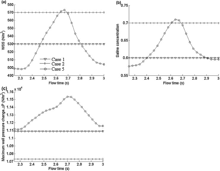
Comparison of results for 6-mm diameter vessel with uniform and pulsatile blood flow rates: (a) distribution of maximum WSS on the blood vessel wall, (b) distribution of maximum saline concentration on the blood vessel wall, and (c) maximum wall pressure change on the blood vessel wall along the flow direction.

Figure 8(b) shows the profile of maximum saline phase concentration on the wall over a period. As seen in Figure 8(b), the maximum saline phase concentrations for constant low and high blood flow rates are 0.7 and 0.6 respectively where it varies from 0.58 to 0.71 in pulsatile flow. So, the deviations of the calculated maximum wall concentration from those for the maximum and minimum blood flow rates are about 1:5% and 3% respectively when we assume the flow to be steady instead of pulsatile. This indicates that the pulsatile nature of the blood flow does not have much effect on the clearance of the blood cells in the field of view.

The effects of the pulsatile blood flow on the wall pressure are shown in Figure 8(c), which shows that the maximum wall pressure change (ΔP) remains constant for both higher and lower blood flow rates. The values of ΔP for the higher and lower blood flow rates are 11,100 and 10; 730 N/m², respectively. In the case of the pulsatile flow, ΔP varies between 11,100 and 11; 500 N/m². Another point to note is that ΔP for the pulsatile flow is higher than for the case of higher flow rate for the entire period.

4. CONCLUSIONS

The comparison of the results for Eulerian–Eulerian and mixture models show small difference that suggests that the less computationally expensive and relatively less accurate can be employed for simulation of larger diameter blood vessels where the Fahraeus–Lindqvist effect can be neglected. The current study shows the effect of the possible ranges of parameters that include vessel diameter, blood flow and injection rates on the WSS, clearance of blood on the optical pathway, and wall pressure. Higher injection rate appears to produce better imaging by removing 100% blood cells from jet pathway for a smaller diameter vessel, but it causes a huge jump in both the WSS and wall pressure. The greatest effects on the WSS and wall pressure change are found to be due to changes in the diameter of the blood vessel. We found that when the diameter of the blood vessel is reduced by half, the maximum WSS jumps to 15 times of its original value. The reduction in blood-vessel diameter occurs in stenotic vessels. The second largest effects on the WSS and wall pressure are due to changes in the rate of injection of saline from the catheter tip; when the injection rate is doubled, the maximum WSS becomes 2.5 times of its original value. Pulsatile nature of the blood flow is found to have minimum effects in both WSS and wall pressure change.

It appears from the fluid-structure interaction study by Cho et al. [46] that WSS can be more than 20% higher for deformable vessels, as compared with rigid vessel walls. It would be therefore useful to extend the present study to consider deformable vessels, with a more quantitatively accurate arterial input function for the pulsatile blood flow rate (e.g., as in [55]).

This study can be extended for more intermediate parameter values and a constitutive relationship for the maximum WSS, maximum saline phase concentration on the wall, and the maximum/minimum total pressure on the wall, in terms of the blood-vessel diameter, injection rate, and blood flow rate.

References

- 1.Drexler W, Morgner U, Kartner FX, Pitris C, Boppart SA, Li XD, Ippen EP, Fujimoto JG. In vivo ultrahigh-resolution optical coherence. Optics Letters. 1999;24(17):1221–1223. doi: 10.1364/ol.24.001221. [DOI] [PubMed] [Google Scholar]
- 2.Huang D, Swanson EA, Lin CP, Schuman JS, Stinson WG, Chang W, Hee MR, Flotte T, Gregory K. Optical coherence tomography. Science (New York NY) 1991;254(5035):1178–1181. doi: 10.1126/science.1957169. [DOI] [PMC free article] [PubMed] [Google Scholar]
- 3.Cheng H, Luo Q, Zeng S, Chen S, Cen J, Gong H. Modified laser speckle imaging method with improved spatial resolution. Journal of Biomedical Optics. 2003;8(3):559–564. doi: 10.1117/1.1578089. [DOI] [PubMed] [Google Scholar]
- 4.Kolkman RGM, Hondebrink E, Steenbergen W. In vivo photoacoustic imaging of blood vessels using an extreme-narrow aperture sensor. IEEE Journal of Selected Topics in Quantum Electronics. 2003;9(2):343–346. [Google Scholar]
- 5.Xu M, Wang LV. Photoacoustic imaging in biomedicine. Review of Scientific Instruments. 2006;77(4):041101–22. [Google Scholar]
- 6.Yang D, Xing D, Gu H, Tan Y, Zeng L. Fast multielement phase-controlled photoacoustic imaging based on limited-field-filtered back-projection algorithm. Applied Physics Letters. 2005;87(19):194101–3. [Google Scholar]
- 7.Deckelbaum LI, Stetz ML, O’Brien KM, Cutruzzola FW, Gmitro AF, Laifer LI, Gindi GR. Fluorescence spectroscopy guidance of laser ablation of atherosclerotic plaque. Lasers in Surgery and Medicine. 1989;9(3):205–214. doi: 10.1002/lsm.1900090303. [DOI] [PubMed] [Google Scholar]
- 8.Lakowicz JR. Principles of Fluorescence Spectroscopy. Kluwer Academic/Plenum; New York: 1999. [Google Scholar]
- 9.Mahadevan-Jansen A, Mitchell MF, Ramanujamf N, Malpica A, Thomsen S, Utzinger U, Richards-Kortumt R. Nearinfrared raman spectroscopy for in vitro detection of cervical precancers. Photochemistry and Photobiology. 1998;68(1):123–132. doi: 10.1562/0031-8655(1998)068<0123:nirsfv>2.3.co;2. [DOI] [PubMed] [Google Scholar]
- 10.Marcu L. Fluorescence lifetime in cardiovascular diagnostics. Journal of Biomedial Optics. 2010;15(1):011106–10. doi: 10.1117/1.3327279. [DOI] [PMC free article] [PubMed] [Google Scholar]
- 11.Richards-Kortum R, Sevick-Muraca E. Quantitative optical spectroscopy for tissue diagnosis. Annual Review of Physical Chemistry. 1996;47:555–606. doi: 10.1146/annurev.physchem.47.1.555. [DOI] [PubMed] [Google Scholar]
- 12.Wagnieres GA, Star WM, Wilson BC. In vivo fluorescence spectroscopy and imaging for oncological applications. Photochemistry and Photobiology. 1998;68(5):603–632. [PubMed] [Google Scholar]
- 13.Xie C, Dinno MA, Li Y. Near-infrared raman spectroscopy of single optically trapped biological cells. Optics Letters. 2002;27(4):249–251. doi: 10.1364/ol.27.000249. [DOI] [PubMed] [Google Scholar]
- 14.Ergu̇l O, Arslan-Ergu̇l A, Gu̇ṙel L. Rigorous solutions of scattering problems involving red blood cells. Proceedings of the Fourth European Conference; Barcelona. 2010; pp. 1–4. [Google Scholar]
- 15.Turcu I, Pop CVL, Neamtu S. High-resolution angle-resolved measurements of light scattered at small angle by red blood cells in suspension. Applied Optics. 2006;45(9):1964–1971. doi: 10.1364/ao.45.001964. [DOI] [PubMed] [Google Scholar]
- 16.Moreno PR, Muller JE. Identification of high-risk atherosclerotic plaques: a survey of spectroscopic methods. Current Opinion in Cardiology. 2002;17(6):638–647. doi: 10.1097/00001573-200211000-00010. [DOI] [PubMed] [Google Scholar]
- 17.Virmani R, Burke AP, Kolodgie FD, Farb A. Vulnerable plaque: the pathology of unstable coronary lesions. Journal of Interventional Cardiology. 2002;15(6):439–446. doi: 10.1111/j.1540-8183.2002.tb01087.x. [DOI] [PubMed] [Google Scholar]
- 18.Waxman S, Ishibashi F, Muller JE. Detection and treatment of vulnerable plaques and vulnerable patients: novel approaches to prevention of coronary events. Circulation. 2006;114(22):2390–2411. doi: 10.1161/CIRCULATIONAHA.105.540013. [DOI] [PubMed] [Google Scholar]
- 19.Naghavi M, Libby P, Falk E, Casscells SW, Litovsky S, Rumberger J, Badimon JJ, Stefanadis C, Moreno P, Pasterkamp G, Fayad Z, Stone PH, Waxman S, Raggi P, Madjid M, Zarrabi A, Burke A, Yuan C, Fitzgerald PJ, Siscovick DS, de Korte CL, Aikawa M, Airaksinen KEJ, Assmann G, Becker CR, Chesebro JH, Farb A, Galis ZS, Jackson C, Jang IK, Koenig W, Lodder RA, March K, Demirovic J, Navab M, Priori SG, Rekhter MD, Bahr R, Grundy SM, Mehran R, Colombo A, Boerwinkle E, Ballantyne C, Insull W, Schwartz RS, Vogel R, Serruys PW, Hansson GK, Faxon DP, Kaul S, Drexler H, Greenland P, Muller JE, Virmani R, Ridker PM, Zipes DP, Shah PK, Willerson JT. From vulnerable plaque to vulnerable patient: a call for new definitions and risk assessment strategies: part I. Circulation. 2003;108(14):1664–1672. doi: 10.1161/01.CIR.0000087480.94275.97. [DOI] [PubMed] [Google Scholar]
- 20.Casscells W, Hathorn B, David M, Krabach T, Vaughn WK, McAllister HA, Bearman G, Willerson JT. Thermal detection of cellular infiltrates in living atherosclerotic plaques: possible implications for plaque rupture and thrombosis. Lancet. 1996;347:1447–1449. doi: 10.1016/s0140-6736(96)91684-0. [DOI] [PubMed] [Google Scholar]
- 21.Christov A, Dai E, Drangova M, Liu LY, Abela GS, Nash P, McFadden G, Lucas A. Optical detection of triggered atherosclerotic plaque disruption by fluorescence emission analysis. Photochemistry and Photobiology. 2000;72(2):242–252. doi: 10.1562/0031-8655(2000)072<0242:odotap>2.0.co;2. [DOI] [PubMed] [Google Scholar]
- 22.Daniel TB, Akins EW, Hawkins IF. A solution to the problem of high-flow jets from miniature angiographic catheters. AJR. 1990;154:1091–1095. doi: 10.2214/ajr.154.5.2108548. [DOI] [PubMed] [Google Scholar]
- 23.Coelho SLV, Hunt JCR. The dynamics of the near field of strong jets in crossflows. Journal of Fluid Mechanics. 1989;200:95–120. [Google Scholar]
- 24.Foust J, Rockwell D. Structure of the jet from a generic catheter tip. Experiments in Fluids. 2006;41(4):543–558. [Google Scholar]
- 25.Pope SB. Turbulent Flows. Cambridge University Press; Cambridge, UK: 2000. [Google Scholar]
- 26.Broadwell JE, Breidenthal RE. Structure and mixing of a transverse jet in incompressible flow. Journal of Fluid Mechanics. 1984;148:405–412. [Google Scholar]
- 27.Plesniak MW, Cusano DM. Scalar mixing in a confined rectangular jet in crossflow. Journal of Fluid Mechanics. 2005;524:1–45. [Google Scholar]
- 28.Sherif SA, Pletcher RH. Measurements of the flow and turbulence characteristics of round jets in crossflow. Journal of Fluids Engineering. 1989;111:165–171. [Google Scholar]
- 29.Smith SH, Mungal MG. Mixing, structure and scaling of the jet in crossflow. Journal of Fluid Mechanics. 1998;357:83–122. [Google Scholar]
- 30.Su LK, Mungal MG. Simultaneous measurements of scalar and velocity field evolution in turbulent crossflowing jets. Journal of Fluid Mechanics. 2004;513:1–45. [Google Scholar]
- 31.Weber PW, Coursey CA, Howle LE, Nelson RC, Nichols EB, Schindera ST. Modifying peripheral IV catheters with side holes and side slits results in favorable changes in fluid dynamic properties during the injection of iodinated contrast material. AJR. 2009;193:970–977. doi: 10.2214/AJR.09.2521. [DOI] [PubMed] [Google Scholar]
- 32.Varghese SS, Frankel SH. Numerical modeling of pulsatile turbulent flow in stenotic vessels. Journal of Biomechanical Engineering. 2003;125(4):445–460. doi: 10.1115/1.1589774. [DOI] [PubMed] [Google Scholar]
- 33.Orszag SA, Yakhot V, Flannnery WS, Boysan F, Chowdhury D, Maruzewski J, Patel B. Renormalization group modeling and turbulence simulations. International Conference on Near-Wall Turbulent Flows; Tempe, Arizona. 1993; pp. 1031–1046. [Google Scholar]
- 34.Ghata N, Aldredge RC, Bec J, Marcu L. Towards development of an intravascular diagnostic catheter based on fluorescence lifetime spectroscopy: study of an optimized blood flushing system. SPIE 7883, Photonic Therapeutics and Diagnostics VII San Fransisco; CA. 2011; pp. 1–13. [Google Scholar]
- 35.ANSYS. Fluent User Manuals V12.1. ANSYS, Inc.; Cannosburg, PA, USA: 2010. [Google Scholar]
- 36.Haynes RH. Physical basis of the dependence of blood viscosity on tube radius. American Journal of Physiology. 1960;198:1193–1205. doi: 10.1152/ajplegacy.1960.198.6.1193. [DOI] [PubMed] [Google Scholar]
- 37.Merrill EW, Cokelet GR, Britten A, Wells RE. Non-Newtonian rheology of human blood – effect of fibrinogen deduced by subtraction. Circulation Research. 1963;13:48–56. doi: 10.1161/01.res.13.1.48. [DOI] [PubMed] [Google Scholar]
- 38.Charm SE, Kurland GS. Blood Rheology and Cardiovascular Fluid Dynamics. Academic Press; London: 1965. [Google Scholar]
- 39.Cokelet GR. The Rheology of Human Blood: In Biomechanics. Prentice Hall; Englewood Cliffs, NJ: 1972. [Google Scholar]
- 40.Fournier RL. Basic Transport Phenomena in Biomedical Engineering. Taylor & Francis; New York: 2006. [Google Scholar]
- 41.Srivastava VP. A theoretical model for blood flow in small vessels. International Journal of Application and Applied Mathematics. 2007;2(1):51–65. [Google Scholar]
- 42.Haynes RH, Burton AC. Role of non-Newtonian behavior of blood in hemodynamic. American Journal of Physiology. 1959;197:943–952. doi: 10.1152/ajplegacy.1959.197.5.943. [DOI] [PubMed] [Google Scholar]
- 43.Jung J, Lyczkowski RW, Panchal CB, Hassanein A. Multiphase hemodynamic simulation of pulsatile flow in a coronary artery. Journal of Biomechanics. 2006;39(11):2064–73. doi: 10.1016/j.jbiomech.2005.06.023. [DOI] [PubMed] [Google Scholar]
- 44.Qiu Y, Tarbell JM. Interaction between wall shear stress and circumferential strain affects endothelial cell biochemical production. Journal of Vascular Research. 2000;37:147–157. doi: 10.1159/000025726. [DOI] [PubMed] [Google Scholar]
- 45.Wootton DM, Ku DN. Fluid mechanics of vascular systems, diseases and thrombosis. Annual Review of Biomedical Engineering. 2002;1:299–329. doi: 10.1146/annurev.bioeng.1.1.299. [DOI] [PubMed] [Google Scholar]
- 46.Cho SW, Kim SW, Sung MH, Ro KC, Ryou HS. Fluid-structure interaction analysis on the effects of vessel material properties on blood flow characteristics in stenosed arteries under axial rotation. Korea-Australia Rheology Journal. 2010;23(1):7–16. [Google Scholar]
- 47.Picart A, Berlemont A, Gouesbet G. Modeling and predicting turbulence fields and dispersion of discrete particles transported by turbulent flows. International Journal of Multiphase Flow. 1986;12(2):237–261. [Google Scholar]
- 48.Simonin O. Eulerian Formulation for Particle Dispersion in Turbulent Two-Phase Flows. Erlangen, FRG. Jülich: Kernforschungsanlage Jülich; 1990. [Google Scholar]
- 49.Clift R, Weber ME. Bubbles, Drops, and Particles. Academic Press; London: 1978. [Google Scholar]
- 50.Vignon-Clementel IE, Figueroa CA, Jansen KE, Taylor CA. Outflow boundary conditions for 3D simulations of nonperiodic blood flow and pressure fields in deformable arteries. Computer Methods in Biomechanics and Biomedical Engineering. 2010;125(4):1–16. doi: 10.1080/10255840903413565. [DOI] [PubMed] [Google Scholar]
- 51.Cousins W, Gremaud PA, Tartakovsky M. A new physiological boundary condition for hemodynamics. Journal of Applied Mathematics. 2013;73(3):1203–1223. [Google Scholar]
- 52.Hassan T, Ezura M, Timofeev EV, Tominaga T, Saito T, Takahashi A, Takayama K, Yoshimoto T. Computational simulation of therapeutic parent artery occlusion to treat giant vertebrobasilar aneurysm. AJNR. 2004;25:63–68. [PMC free article] [PubMed] [Google Scholar]
- 53.Olufsen MS. Structured tree outflow condition for blood in larger systemic arteries. American Journal of Physiology. 1999;276:H257–H268. doi: 10.1152/ajpheart.1999.276.1.H257. [DOI] [PubMed] [Google Scholar]
- 54.Yilmaz F, Kutlar AI, Gu H, Tan Y, Gundogdu MYL. Analysis of drag effects on pulsatile blood flow in a right coronary artery by using Eulerian multiphase model. Korea-Australia Rheology Journal. 2011;23(2):89–103. [Google Scholar]
- 55.Sweetman B, Linninger AA. Cerebrospinal fluid flow dynamics in the central nervous system. Annals of Biomedical Engineering. 2011;39(1):484–496. doi: 10.1007/s10439-010-0141-0. [DOI] [PubMed] [Google Scholar]