The Diffusion Model Is Not a Deterministic Growth Model: Comment on Jones and Dzhafarov (2014)

Abstract

Jones and Dzhafarov (2014) claim that several current models of speeded decision making in cognitive tasks, including the diffusion model, can be viewed as special cases of other general models or model classes. The general models can be made to match any set of response time (RT) distribution and accuracy data exactly by a suitable choice of parameters and so are unfalsifiable. The implication of their claim is that models like the diffusion model are empirically testable only by artificially restricting them to exclude unfalsifiable instances of the general model. We show that Jones and Dzhafarov’s argument depends on enlarging the class of “diffusion” models to include models in which there is little or no diffusion. The unfalsifiable models are deterministic or near-deterministic growth models, from which the effects of within-trial variability have been removed or in which they are constrained to be negligible. These models attribute most or all of the variability in RT and accuracy to across-trial variability in the rate of evidence growth, which is permitted to be distributed arbitrarily and to vary freely across experimental conditions. In contrast, in the standard diffusion model, within-trial variability in evidence is the primary determinant of variability in RT. Across-trial variability, which determines the relative speed of correct responses and errors, is theoretically and empirically constrained. Jones and Dzhafarov’s attempt to include the diffusion model in a class of models that also includes deterministic growth models misrepresents and trivializes it and conveys a misleading picture of cognitive decision-making research.

Currently, successful models of speeded, two-choice decision making in cognitive tasks assume that decisions are based on the cumulative evidence obtained from processing a stimulus and that the amount of evidence needed to choose between the alternatives is determined by a response criterion. The time taken to make a decision and the decision that is made depend jointly on the rate at which evidence grows and the settings of the response criteria. The models attribute trial-to-trial variability in response time (RT) and accuracy either to moment-to-moment variability in the evidence, trial-to-trial variability in decision criteria, the rate of evidence growth, or some combination of these sources of variability.

Historically, the largest and most important class of cognitive decision-making models has been the class of sequential-sampling models (Luce, 1986; Townsend & Ashby, 1983; Vickers, 1979). These models assume that there are noisy, moment-to-moment fluctuations in the evidence entering the decision process over the course of a trial, which are modeled mathematically as a stochastic process. Decisions are made by accumulating successive samples of noisy evidence to a criterion. This class of models includes the diffusion model (Ratcliff, 1978; Ratcliff & McKoon, 2008), the random-walk models (Laming, 1968; Link & Heath, 1975), the Ornstein-Uhlenbeck model (Busemeyer & Townsend, 1992, 1993), the recruitment or simple accumulator model (Audley & Pike, 1965; LaBerge, 1962), the Vickers or strength accumulator model (Smith & Vickers, 1988; Vickers, 1970), the Poisson counter model (Townsend & Ashby, 1983), the leaky competing accumulator model (Usher & McClelland, 2001), and others. A smaller class of models assumes that evidence growth is deterministic and that variability enters the process only on a trial-to-trial basis, either in the rate of evidence growth, or the settings of the decision criteria, or the starting point for evidence growth. This class includes the Grice model (Grice, 1968, 1972; Grice, Nullmeyer, & Spiker, 1982) and the linear ballistic accumulator (LBA) model (Brown & Heathcote, 2008).

One of the most successful and widely studied models of two-choice decision making is Ratcliff’s diffusion model (Ratcliff, 1978; Ratcliff & McKoon, 2008). This model assumes that the decision process accumulates successive estimates of the relative strength of evidence for the two choices until the cumulative difference in evidence favoring one alternative over the other reaches a criterion. The accumulating evidence is modeled as a Wiener, or Brownian motion, diffusion process (Cox & Miller, 1965; Karlin & Taylor, 1981), and the criteria are modeled as upper and lower boundaries on the cumulative evidence. The rate of evidence growth is represented by the drift of the diffusion process. In the diffusion model, variability in RTs and choice probabilities across conditions is attributed to moment-to-moment variability in the accumulation of evidence (within-trial variability) and to trial-to-trial variability in the starting point for evidence growth and the rate of evidence growth. The model explains how choice probabilities and the location, dispersion, and shape of RT distributions for correct responses and errors vary with stimulus discriminability, response bias, and speed–accuracy tradeoff settings (Ratcliff, 1978; Ratcliff & McKoon, 2008; Ratcliff & Rouder, 1998; Ratcliff & Smith, 2004).

Jones and Dzhafarov (2014) argue that several current cognitive decision-making models, including the diffusion model, the LBA model, and the Grice model, can be viewed as special cases of other, general models or model classes. General models are obtained by discarding all of the assumptions about sources of variability in the models and how variability is constrained across experimental conditions, and retaining only assumptions about model architecture. The main result in Jones and Dzhafarov’s article is that the general models are unfalsifiable, in the sense that unfalsifiable instances of them can always be found. Rather than being viewed as empirically testable and falsifiable, Jones and Dzhafarov argue that the general models should be viewed as “universal modeling languages” for describing data. A universal modeling language for a cognitive decision-making model is simply a redescription of the observed data in the language of evidence growth and response criteria, as these constructs are represented in the architecture of the particular model. In the absence of any a priori theoretical constraints on how evidence and criteria are distributed within and across trials, it is always possible to find a description of performance in these terms that matches the data exactly and, moreover, it is possible to translate freely from one such description to another.

Jones and Dzhafarov (2014) argue that the only real content possessed by cognitive decision-making models is contained in their “technical” assumptions about the sources of variability and how they are distributed, together with their assumptions about selective influence, that is, how the model’s parameters are constrained across experimental conditions. They argue that it is the combination of technical assumptions and selective influence assumptions, not the model architecture, that serves to define classes of falsifiable models, because it is these assumptions that distinguish falsifiable instances of the general models from unfalsifiable instances. According to them, the falsifiability of the models depends wholly on a set of assumptions that are auxiliary to, and logically independent of, a model, rather than being part of its essential structure.

Jones and Dzhafarov (2014) are also critical of the technical and selective influence assumptions that have been used to fit models in the literature, arguing that neither set of assumptions is well-motivated theoretically. The implication of their argument is that the apparent testability and falsifiability of current models may be little more than an artifact of the restrictions that have been imposed on the general models in order to exclude their unfalsifiable instances. Because the general models are essentially interchangeable as descriptions of data, the further implication of their argument is that any debate about competing model architectures is, at least within the set of models considered in their article, simply an argument about language, rather than about psychological processes. A researcher’s choice of model becomes essentially an arbitrary one, with no more scientific content than, say, the decision to talk about a scientific phenomenon in English rather than French or German. Under these circumstances, fits of models to data can provide little insight into the processes that are actually involved in decision making.

In this comment, we focus specifically on Jones and Dzhafarov’s (2014) claims about the diffusion model. The diffusion model is a sequential-sampling model and so differs from both the Grice model and the LBA model in its assumption of within-trial variability in evidence accumulation. Importantly, unlike the Grice model and LBA model, the stochastic properties of this variability are the basis of the diffusion model’s predictions about RT distributions. Although the model also assumes across-trial variability in drift rates and starting points, the predicted shapes of RT distributions in the model are determined primarily by within-trial variability. Consequently, the properties of the model can only be understood by understanding the particular way in which within-trial variability in accumulating evidence predicts trial-to-trial variability in speed and accuracy.

We show that Jones and Dzhafarov’s (2014) claims about the unfalsifiability of diffusion models depend on enlarging the class of “diffusion” models to include models in which there is, in fact, no diffusion. Jones and Dzhafarov denote this enlarged class by gDM, for general diffusion model. The unfalsifiable instances of gDM are models in which there is little or no within-trial variability and in which all of the variability in RT and accuracy is attributed to across-trial variability in the rate of evidence accumulation. Although gDM has the same architecture as Ratcliff’s diffusion model (two decision boundaries and a single evidence total), the use of the term “diffusion model” to describe models from which diffusive variability has been largely or wholly eliminated is likely to mislead all but the most attentive reader. Nevertheless, to help readers relate our comments to the arguments in Jones and Dzhafarov’s article we have retained their gDM terminology to denote the enlarged class of models.

In this comment, we make seven points and then expand on them in later sections:

1. Jones and Dzhafarov’s (2014) “universal modeling language” for diffusion models is unrelated to either the physical theory or the mathematical analysis of diffusion processes. It is, rather, just a restatement of the elementary law of kinematics relating distance, velocity, and time. This law describes a deterministic linear growth process from which within-trial stochastic variability in evidence accumulation has been excluded. Consequently, it is unable to characterize the properties of models with stochastic evidence growth. The unfalsifiable members of gDM are deterministic linear growth models and a subset of models that are close to it in parameter space. We refer to the deterministic growth model as detDM, for “deterministic diffusion model.” We emphasize that, unlike the standard diffusion model and other members of gDM, deterministic growth models have no within-trial variability.¹

2. In detDM, all of the trial-to-trial variability in RT and accuracy depends on the distributions of across-trial variability in the rate of evidence growth. The model is universal and unfalsifiable, because without within-trial variability, the distributions of evidence growth, that is, the drift rates, can be chosen arbitrarily to match the data exactly.

3. The analysis of RT distributions and accuracy using detDM leads to implausibly complex, bimodal, across-trial distributions of drift rates. We characterize the properties of detDM in detail in order to show the ways in which it differs fundamentally from the standard diffusion model.

4. Jones and Dzhafarov (2014) show that, even with nonzero within-trial variability, gDM is still either universal and unfalsifiable, or else minimally constraining. This result depend on setting the amount of within-trial variability to be sufficiently small that the model’s predictions differ in only minor ways from those of detDM.

5. Whereas detDM with arbitrary drift rate distributions is universal and unfalsifiable, the standard diffusion model is highly constrained by the effects of within-trial variability and predicts RT distributions that have a particular characteristic form. The model is unable to predict distributions that do not have this form.

6. In the standard diffusion model, there is across-trial variability in drift rate and in the starting point for evidence accumulation relative to the decision boundaries. The distributions of drift rates and starting points have specific, theoretically constrained forms. This variability leads to differences in the relative speeds of correct responses and errors but leaves the shapes of the predicted RT distributions largely unchanged.

7. In the standard diffusion model, drift rates are assumed to be unaffected by manipulations that affect decision boundaries, such as speed/accuracy instructions or bias manipulations. Decision boundaries are assumed to be unaffected by manipulations that affect drift rate, like stimulus discriminability. These assumptions about parameter invariance are criticized by Jones and Dzhafarov (2014) as being overly restrictive. We argue instead that they are theoretically principled and therefore possess explanatory power. They also provide powerful constraints for model testing, but they are (of course) amenable to revision or modification if warranted by data.

We expand on these points in the following sections.

1. The Universal Modeling Language for Diffusion Models Describes a Deterministic Evidence Growth Process

Jones and Dzhafarov’s (2014) “universal modeling language” for diffusion models, which defines the model detDM and which is characterized in their Theorem 10, is just a restatement of the elementary law of kinematics relating distance (a), velocity (v), and time (T),

$$T=\frac{a}{v}.$$ (1)

The unfalsifiable (and hence universal) members of gDM are the model detDM and models that are close to it in parameter space.² In Jones and Dzhafarov’s application of Equation 1, velocity becomes drift rate or rate of evidence growth and distance becomes the distance from the starting point to a boundary or criterion. If the starting-point-to-boundary distance is a and the drift rate is v, then the response time is a/v. Because evidence growth is deterministic, there is a one-to-one correspondence between drift rates (v) and RTs (T): Every different drift rate results in a different RT and, conversely, if two RTs are different then their drift rates must have been different, as shown in the top panel of Figure 1. If the RT (or more precisely, the decision time) is T, then the drift rate, v, must have been a/T. The distance traveled or the speed of travel or both may vary randomly from trial to trial, but there is no moment-to-moment variability in the process itself.³ Jones and Dzhafarov’s argument about the unfalsifiability of the class gDM relies on the possibility of enlarging the class of diffusion models to include detDM.

Figure 1.

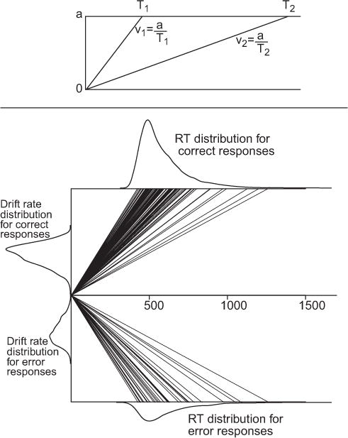
The top panel illustrates the deterministic growth model of Equation 1, including the one-to-one correspondence between time and velocity (drift rate). The distribution of velocities is fixed by the distribution of times because each time, T₁ and T₂, is uniquely associated with a particular velocity, v₁ and v₂. The bottom panel shows an example of correct and error response time (RT) distributions generated by the standard diffusion model (horizontal axes) and the distribution of drift rates in the deterministic model needed to produce them (vertical axis). The parameters of the diffusion model used to generate the simulated RT distributions were a = 0.12, T_er = 0.4, z = 0.06, η = 0.12, s_z = 0.02, s_t = 0.1, and v = 0.2.

The model detDM has the same architecture as the diffusion model but has no within-trial variability. Like the diffusion model, drift rates can be positive or negative: positive rates represent evidence for one alternative; negative rates represent evidence for the other alternative. Also like the diffusion model, a response is made when the cumulative evidence reaches either an upper or lower boundary. In detDM, however, the evidence only increases or decreases, but it does not do both, because there is no stochastic variability during a trial. Because there is a one-to-one correspondence between drift rates and RTs in detDM, the predicted probability of a response at the upper boundary is equal to the probability that the drift rate on a trial is positive. In the universal modeling language for diffusion models, this probability can be chosen to match the data exactly.

2. The Model detDM Misrepresents the Diffusion Model

In the standard diffusion model, the accumulated evidence on any trial depends jointly on the drift rate, v, which varies from trial to trial, and the within-trial, stochastic variability in the evidence process, which varies from moment to moment. The amount of within-trial variability is controlled by the infinitesimal standard deviation of the diffusion process, s. The square of the infinitesimal standard deviation, s², is termed the diffusion coefficient. In Jones and Dzhafarov’s (2014) article, drift is denoted k, and the diffusion coefficient is denoted σ². Their claim that gDM is universal and unfalsifiable is based on the properties of the deterministic growth model detDM, as described in the previous section and expressed in their Equation 2.12. Apart from differences in notation, this equation is just Equation 1 above.

Mathematically, a straight line with no moment-to-moment stochastic variability is not a diffusion process—except in the trivial sense that a constant function is a stochastic process. Karlin and Taylor (1981, p. 166), for example, stated that, for the purposes of applications (i.e., excluding special or degenerate cases), a diffusion process is a continuous-time, continuous-state Markov process with σ² > 0, that is, with a strictly positive diffusion coefficient. Most of the theoretically interesting properties of diffusion processes as models of decision making are not shared by the deterministic model. The most basic of these properties is that the diffusion model predicts trial-to-trial variability in RTs and errors through within-trial variability in the evidence accumulation process for single values of drift rate. Mean drift rate is the only parameter of the model that changes across conditions with varying stimulus strength or discriminability. In contrast, the deterministic model predicts the same response and the same RT on every trial. Consequently, all of the predictive work in the deterministic model is done by trial-to-trial variability in drift rate or by other components of processing that vary across trials.

The behavior of the deterministic model of Equation 1 is shown in Figure 1. As shown in the top panel, the deterministic model attributes different decision times, T₁ and T₂, to differences in drift or growth rates, v₁ and v₁. (Essentially the same argument can be made with a single drift rate and trial-to-trial variation in the distance to the boundaries.) Unlike the diffusion model, a different value of v is needed for every response/RT combination. Indeed, as Jones and Dzhafarov (2014) recognize, in detDM the distance to the boundaries can be set to unity with the other parameters scaled appropriately. Their “universal modeling language” then reduces to the theoretically empty statement that speed is proportional to the reciprocal of time and that distributions of RTs can also be described as distributions of response speeds. In essence, their unfalsifiable “diffusion” model—which is the theoretically important member of the model class gDM for their argument—is a model from which all of the within-trial variability has been stripped out and its effects replaced by between-trial variability, chosen in such a way as to match the data. Unlike the LBA and Grice models, in which evidence growth actually is deterministic, the detDM characterization of the diffusion model bears little relationship to the standard model.

3. The Deterministic Model detDM Leads to Implausibly Complex Drift Rate Distributions

Point 2 emphasized that all the predictive work in detDM must be done by across-trial variability in drift rate or other components of processing, because within-trial variability is eliminated from the model. The bottom panel of Figure 1 shows the implications of this aspect of the model. The figure shows the results of applying detDM to RT distributions and choice probabilities generated by a standard diffusion model with parameters representative of fits to empirical data. The distributions plotted on the upper and lower decision boundaries are the joint distributions of correct responses and errors, respectively. The probability mass in each member of a joint distribution pair is the probability of the associated response, so the joint distributions carry information about both RT and choice probabilities. The oblique rays projecting from the starting point at t = 0 to points on the boundaries represent the cumulative evidence for different values of positive and negative v predicted by the deterministic model and the RTs that result. The smoothed drift rate distributions on the vertical (evidence) axis are the drift rate distributions needed to obtain the observed RT distributions for the boundary separation shown. As described in Point 1, a different v is needed for every different RT in each of the two distributions.

As the figure shows, detDM provides no insight into the processes that underlie RT and accuracy, because it is simply a redescription of the data in different language. As a result, it leads to distributions of drift rates that are as complex as the original data. The implied distribution of drift rates is bimodal with a pair of lobes that are roughly mirror images of each other. The lobes have the opposite skew to the distributions of RT: Right-skewed RT distributions produce distributions whose positive and negative lobes are both skewed toward zero. The probability masses in the positive and negative lobes are equal to the observed probabilities of correct responses and errors, respectively. To prove the universality of detDM, Jones and Dzhafarov (2014) allow the properties of the drift rate distribution and the probability masses in its two lobes to differ freely between each condition of the experiment, because they view any constraints on the drift rate as “technical” assumptions that are not a core part of the model architecture.

Figure 2 shows three different (smoothed) distributions of evidence from application of detDM to data simulated from a standard diffusion model with drift rates 0, 0.2, and 0.4. Empirically, these three pairs correspond to experimental conditions with low, medium, and high accuracy. The lobes on the left are the drift rates for errors; the lobes on the right are the drift rates for correct responses. As the previous paragraph pointed out, different drift rate distributions with different probability masses in their pairs of lobes are required to describe the RT distributions in each of the three conditions. Because the deterministic model is atheoretical, it provides no insight into why the distributions should be so complex or why they should vary in shape in the ways they are required to vary across conditions.

Figure 2.

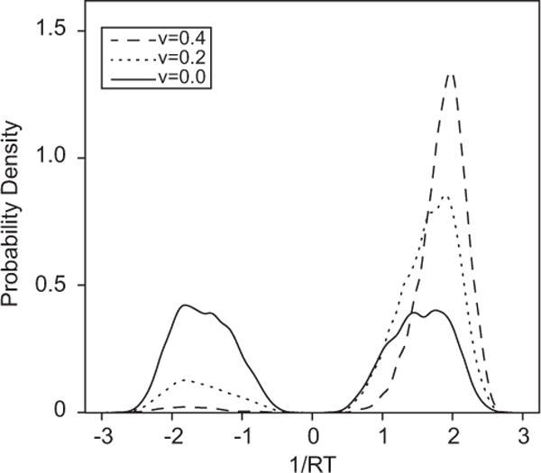
Examples of the drift rate distributions for the deterministic model derived from response time (RT) distributions for the diffusion model. The drift rates for the diffusion model were 0.0, 0.2, and 0.4; the other parameters were the same as in Figure 1. The positive lobes of the drift rate distributions describe the distributions of correct responses and the negative lobes describe the distributions of errors. The proportions of probability mass in the positive lobes are the proportions of correct responses. Separate drift rate distributions, with different shapes and different proportions of mass in their positive and negative lobes, are needed for each value of drift rate.

Even as a purely empirical description of performance, the model provides no parsimony or data reduction, because it requires as many free parameters to describe the distributions of evidence as are needed to describe the original data. An exact description of the data would need as many parameters as there are data points because every different RT requires a different value of v. A description that does not seek to characterize the data exactly, but only to provide a smoothed approximation to them using standard, goodness-of-fit criteria (e.g., maximum likelihood or minimum chi-square) would need as many parameters as are required to provide a description of a pair of distributions with varying location, dispersion, shape, and probability mass in each condition. Moreover, the claimed universality of the model breaks down whenever there is a requirement that the distributions of drift rates be the same in two or more conditions: for example, if the same stimulus is presented under both speed and accuracy instructions.

For Jones and Dzhafarov (2014), the lack of theoretical content in detDM is not an issue. Indeed, they would probably argue that it is precisely their point, because the theoretical emptiness of detDM that we have emphasized here follows from its universality, which they proved. Jones and Dzhafarov seek to establish detDM as a legitimate special case of gDM that has been excluded from the class of diffusion models only by virtue of the latter’s arbitrary and poorly motivated constraints on the distributions of evidence growth. The implication of this line of argument is, of course, that the diffusion model is preserved from triviality only by virtue of its arbitrary evidence growth and selective influence assumptions.

Our purpose here in highlighting the properties of the deterministic model detDM is to illustrate for the reader just how different its properties are to those of the standard diffusion model, despite the models sharing a name and a common architecture and purportedly belonging to the same general model class. Unlike Jones and Dzhafarov (2014), we view the theoretical emptiness of detDM as an object lesson in the hazards of attempting to identify a model with only a restricted subset of its defining assumptions. As we discuss in more detail subsequently, we believe that assumptions about sources of variability and how they are constrained across conditions need to be viewed as integral parts of a model and not as, in effect, afterthoughts. The fact that one may wish selectively to relax or modify some of the assumptions in order to help understand some particular data set should not be viewed as a violation of this principle.

4. The Claimed Universality of the General Diffusion Model gDM Depends on Making Within-Trial Variability Negligible

Jones and Dzhafarov (2014) also claim that, even with nonzero within-trial variability, the diffusion model is either universal or else minimally constraining and offer two arguments to support their claim. Both of these arguments, although they ostensibly involve fixing the diffusion coefficient to some specified, nonzero value, actually involve rescaling the other parameters of the model in order to make the effects of within-trial variability negligible or else comparatively small. Consequently, their universal diffusion model with nonzero within-trial variability does not differ in any theoretically meaningful way from the deterministic model detDM, whose properties we have already characterized. The conditions needed to reduce the diffusion model with nonzero within-trial variability to the deterministic model are prohibited in the standard diffusion model, which precludes bimodal distributions of drift, but Jones and Dzhafarov relegate these constraints to the category of “technical assumptions.”

Jones and Dzhafarov’s (2014) first argument is contained in their Theorem 12, which asserts that the joint distributions of RT predicted by a diffusion model with a fixed, strictly positive diffusion coefficient (σ² > 0) can be made to agree arbitrarily closely with any pair of empirical, joint RT distributions, by a suitable choice of parameters. The substance of Jones and Dzhafarov’s theorem is simply that the predictions of the diffusion model can be made indistinguishable from those of a deterministic model by setting the effects of within-trial variability to be negligible. The across-trial distributions of drift can then be chosen arbitrarily, as they are in the deterministic model, to match the data exactly. The effects of within-trial variability can be made negligible either by setting the diffusion coefficient to be very small or by setting the other parameters to be very large. Within-trial variability is controlled by the value of σ and becomes negligible as σ approaches zero. By setting σ to some small, but nonzero, value the effects of within-trial variability can be almost completely eliminated from the model.

Exactly the same result can be obtained by fixing σ to some arbitrary, not necessarily small, value and allowing the other parameters in the model to become very large. Like other decision models, the parameters of the diffusion model cannot all be independently estimated from data: The parameters are said to be identified only to the level of a ratio. In order to fit the model to data, it is necessary to assign one of its parameters an arbitrary value and to express the other parameters as multiples of this value. For the diffusion model, the usual practice is to fix σ and to express drift rates and their standard deviations (denoted η) and the decision boundaries as multiples of σ Because the parameters are not uniquely identified, a model with σ = 0.001, v = 0.1, η = 0.1, and a = 0.1 will make exactly the same predictions as one with σ = 0.1, v = 10.0, η = 10.0, and a = 10.0. As a result, it is possible to fix σ to a specified value and to scale the other parameters in such a way that its effect is nevertheless negligible. The properties of the model then differ in only minor ways from those of the deterministic model.

Jones and Dzhafarov’s (2014) second argument is contained in the discussion surrounding their Figure 3A. In Figure 3A, they fix both the infinitesimal standard deviation and the boundary separation to unity and parametrize the time scale of the process to treat the mapping from model time to real time as a free parameter. Their Figure 3A appears to show that the model can generate a wide variety of distributions of RT as drift is varied, even when the infinitesimal standard deviation and the boundary separation are constrained to be equal. They argue that such a model, while not unfalsifiable, is minimally constraining, especially at small values of t, because the predicted RT distributions are probability mixtures of distributions like the ones shown in their figure, which have very different location and scale properties.

Figure 3.

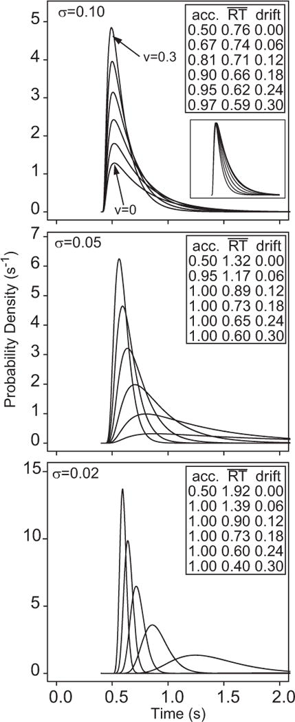
Examples of response time (RT) distributions for correct responses for the standard diffusion model as a function of drift rate (varying from 0 to 0.3 in steps of 0.06) and as a function of the infinitesimal standard deviation (σ = 0.10, 0.05, and 0.02 for the top, middle, and bottom panels, respectively). The inset in the top panel shows the distributions scaled to the same peak value for σ = 0.10. The inset tables show values of accuracy (acc.) and mean RT as a function of drift rate. Only for σ = 0.10 do processes with drift rate greater than zero produce a non-negligible proportion of errors.

What their reparametrization of the time scale obscures, however, is that the example distributions in their Figure 3A have again been drawn from a part of the parameter space in which the effect of within-trial variability is minimal. Although a and σ were both fixed to unity, the time axis in the figure is not t, the time scale of the data, but τ the reparametrized time axis. The relationship between t and τ depends on the ratio a²/σ², the squared boundary separation divided by the diffusion coefficient,

$$t=\left(\frac{a^2}{{\sigma }^2}\right)\tau .$$ (2)

Mapping the distributions in Jones and Dzhafarov’s (2014); Figure 3A to real time—in which mean RTs are typically 350–500 ms or longer—requires an expansion of the time scale by a factor of 10 or more.⁴ This would require that σ² be reduced by a factor of at least 10 relative to a². When σ² is adjusted in this way, the effects of within-trial variability again become minimal. As expected when there is minimal within-trial variability, the error probabilities for the majority of the distribution pairs in Jones and Dzhafarov’s figure are zero or near-zero. Except for the smallest values of drift, the model needs to assume bimodal distributions of drift (k = ±1, ±2, ±4…) to predict RT distributions in which the probability masses are not equal to 1.0 or zero, that is, to generate a range of accuracy values like those found in empirical data. As the caption to their Figure 3 indicates, Jones and Dzhafarov used drifts of + k to generate the RT distributions at the upper boundary and drifts of − k to generate the RT distributions at the lower boundary. The fact that the model predicts error-free performance for most of the drift rates depicted in the figure is obscured by the fact that the distributions have been generated using bimodal distributions of drift and that the RT distributions have been normalized to have the same height.

The effect of progressively reducing within-trial variability by decreasing the diffusion coefficient in the standard model is shown in our Figure 3. For clarity, the predictions of the model are shown in real time (i.e., the time scale of experimental data) rather than in Jones and Dzhafarov’s (2014) reparametrized time scale. This figure shows distributions of RTs for correct responses for a diffusion model generated using parameters typical of those found from fitting empirical data. The error distributions are similar in location and spread to the correct distributions except that their probability masses are smaller (correct and error probability masses must sum to 1). The range of drifts in the standard model was chosen to span a range of accuracy from chance to near-ceiling, and the distributions have been right-shifted by an amount equal to a typical estimate of the nondecision time, T_er. In the standard diffusion model, RT is assumed to be the sum of the decision time, which is the first-passage-time of the diffusion process through a decision boundary, and the time for stimulus encoding, mapping from a stimulus representation to a decision-related representation, response selection, and response execution processes. The value of T_er collectively represents the durations of these other processes.⁵

The families of distributions in the top, middle, and bottom panels of Figure 3 were generated using values of σ of 0.10,0.05, 0.02, respectively, and a boundary separation of a = .12. The value σ = 0.10 is the scaling convention commonly used to fit the model in the cognitive literature. With this choice of σ and a, the model predicts families of distributions like those shown in the upper panel. The accuracy and mean RT associated with each of the distributions in the figure are shown in the insets. The important points to note are, first, that the model is able to predict a full range of accuracy values without variability in drift across trials. Variability in drift is needed only to predict slow errors. Second, the RT distributions it predicts are highly constrained in form. There is little change in the leading edge (the time at which the function first lifts off from zero) or in the mode. The main effect of reducing drift is to increase the concentration of probability mass in the right tail of the distribution, which determines the frequency of slow responses. The invariance of the early part of the RT distribution is shown in the inset to the top panel in Figure 3, in which the RT distributions for σ = 0.10 have been rescaled to all have the same height. The distributions have almost identical modes and left tails; only the right tails differ. This pattern has been found experimentally in numerous applications.

The middle and bottom panels of Figure 3 show the effects of reducing σ to 0.05 and then to 0.02. For σ = 0.05, the invariance of the leading edge and the mode begins to break down and for σ = 0.02 it breaks down completely. The distributions for σ = 0.02 resemble those in Jones and Dzhafarov’s (2014); Figure 3A: Accuracy is at ceiling for all values of drift except v = 0, and there are large shifts in the distribution’s leading edge with increases in drift. In this part of the parameter space the influence of within-trial variability on performance is again minimal and the model approaches the limiting deterministic case. Although such a model can arguably still be called a “diffusion” model, it is not the model in the literature.

5. The Diffusion Model Is Highly Constrained by the Effects of Within-Trial Variability

In Points 1, 2, 3, and 4 we showed that Jones and Dzhafarov’s (2014) claims about the unfalsifiability of gDM rely on them being able to remove within-trial variability from the model and to replace it by arbitrary across-trial distributions in drift. We now show that, unlike the unfalsifiable members of gDM, the standard diffusion model is both highly constrained and highly falsifiable. As we stated earlier, the core assumption of the model, from which its other properties follow, is that within-trial variability in evidence accumulation accounts for both the shapes of RT distributions and the occurrence of errors. Unlike Jones and Dzhafarov’s unfalsifiable universal model, the predicted families of RT distributions for the standard diffusion model are highly constrained (Ratcliff, 2002; Wagenmakers & Brown, 2007). The distribution means and variances and the predicted proportions of correct responses change systematically with changes in drift rate, but the distribution shapes are relatively invariant. This invariance is revealed in quantile-quantile (Q–Q) plots, in which distribution quantiles for processes with different drift rates are plotted against one another. The Q–Q plots for the standard diffusion model are highly linear (Ratcliff & McKoon, 2008; Ratcliff & Smith, 2010), showing that there is relatively little change in distribution shape with changes in drift rate and accuracy, as illustrated by the inset to Figure 3.

Ratcliff (2002) showed that the standard diffusion model was able to fit data from real experiments but could not fit a number of plausible-looking sets of artificial data. His analysis highlighted that the families of RT distributions predicted by the model occupy only a small region of a much larger space of possible experimental outcomes. The model predicts families of RT distributions like those found empirically and, to a large extent, it only predicts these families. This is unlike detDM: Not only does it predict the experimentally observed outcomes, but it also predicts every other outcome as well.

6. The Assumptions About Across-Trial Variability Have Little Effect on the Shapes of the Predicted RT Distributions

It is not correct to suggest, as Jones and Dzhafarov (2014) do, that all of the predictive work in the standard diffusion model is done by auxiliary “technical” assumptions. The standard diffusion model includes one or more sources of across-trial variability, in addition to within-trial variability in the evidence accumulation process, but these sources of variability have little effect on the shapes of the predicted RT distributions. Drift is assumed to be normally distributed with mean ν and standard deviation η; starting point is assumed to be uniformly distributed with mean z and range s_z. The normality of drift rates across trials is similar to the normal distributions of sensory effect of Thurstonian psychophysics and signal detection theory (Green & Swets, 1966; Thurstone, 1927) and can be motivated theoretically in a similar way. Variability in drift rates allows the model to predict errors that are slower than correct responses; variability in starting points allows it to predict errors that are faster than correct responses. Both of these sources of variability express clear theoretical principles. Variability in drift rates expresses the idea that the information from nominally equivalent stimuli differs in quality. Variability in starting points express the idea that the setting of the decision process change from trial to trial.

The same assumptions about the specific forms of across-trial variability are used in most applications of the diffusion model, but these assumptions are not critical to its performance. Ratcliff (2013) showed that the model’s predictions were robust to variations in assumptions about the distributions of drift rates and starting points (see also Ratcliff, 1978, Figure 16). He compared a number of alternative distributions of drift rate and starting point variability and showed that, providing the properties of these distributions were not too extreme, their means and variances were recovered with reasonable accuracy when data simulated from them were fitted with the usual model. Ratcliff’s results further demonstrate that the RT distributions predicted by the model are primarily a function of noisy, within-trial variability in evidence accumulation. Across-trial variability allows it to account for fast errors and/or slow errors but has little effect on the shapes of the predicted RT distributions. Providing that theoretically reasonable constraints are imposed on the distributions of across-trial variability (i.e., symmetry and unimodality), their precise forms are relatively unimportant.

7. Parameter Invariance in the Diffusion Model Follows From Clear Theoretical Principles

Jones and Dzhafarov (2014) are critical of the parameter invariance assumptions made by the diffusion model and the LBA, which they refer to as “selective influence” assumptions. Loosely, these are (a) decision boundaries are not affected by stimulus properties, (b) stimulus or memory processes are not affected by speed–accuracy instructions or bias manipulations, and (c) nondecision times are not affected by either stimulus properties or decision boundaries. Jones and Dzhafarov argue that these assumptions are overly restrictive and suggest reasons for why they might not be expected to hold.

We agree that there are situations in which parameter invariance might not hold. Assumptions about parameter invariance are not inviolable and are not treated as such by researchers in the area; rather, they represent a set of working hypotheses about the processes of speeded decision making. Pragmatically, they represent a powerful set of constraints on a model, which, as a matter of fact, have been satisfied empirically in numerous experimental settings. There are, however, also instances in the literature in which diffusion models making the standard assumptions have failed (Ratcliff & Frank, 2012; Ratcliff & McKoon, 2008, p. 895; Ratcliff & Smith, 2010; Smith & Ratcliff, 2009; Smith, Ratcliff, & Sewell, 2014; Starns, Ratcliff, & McKoon, 2012). In these instances, violation of the assumptions did not lead to a wholesale abandonment of the model but, rather, to a search for new theoretical insights that might explain performance in these particular settings.

This being so, we are puzzled by Jones and Dzhafarov’s (2014) insistence that the standard parameter invariance assumptions are, a priori, inappropriate. We suspect that it is because their claims about universality and unfalsifiability would fail if parameter invariance is assumed, because their results apply only to single experimental conditions; they do not hold when the same set of parameters is required to account for multiple conditions simultaneously.

The Relationship Between gDM, detDM, and the Diffusion Model

In previous sections we have provided a detailed characterization of Jones and Dzhafarov’s model gDM and its distinguished special case, detDM, in which the diffusion coefficient is set to zero. We have emphasized that detDM is unfalsifiable because it is just a redescription of the data in kinematic growth terms. In its most general sense, detDM can simply be viewed as a restatement of the elementary physical fact that speed is proportional to the reciprocal of time. The other unfalsifiable instances of gDM are models that are close to detDM in parameter space and so differ from it in only minor ways. We have provided a detailed characterization of detDM in order to emphasize how fundamentally its properties differ from those of the standard diffusion model—Jones and Dzhafarov’s (2014) “general diffusion model” terminology notwithstanding.

At this point, the reader may be motivated to ask the question: When fitting the diffusion model to data, what ensures that the model you estimate will be a proper diffusion model, with non-negligible within-trial variability, rather than the deterministic model, detDM? To phrase the question in another way, what prevents the free parameters of the model from growing so large that the contributions of the diffusion coefficient become negligible? The most straightforward answer is that these outcomes are prevented by the constraint that the distributions of drift cannot be bimodal. The standard diffusion model makes specific, parametric assumptions about the across-trial distributions of drift, namely, that drift is normally distributed with variance independent of the mean. However, as Ratcliff (2013) showed, it suffices to impose the weaker constraint that the distributions of drift must be unimodal in order to recover model parameters reliably and to exclude deviant special cases like detDM.

We agree with Jones and Dzhafarov (2014) that a diffusion model with arbitrary bimodal distributions of drift would be difficult to falsify. Falsification under these circumstances would depend largely on the constraints imposed by the selective influence assumptions, as they assert. Arguably, then, a contribution of their article is that they have highlighted that the falsifiability of the diffusion model relies on a set of assumptions that must be strong enough to preclude arbitrary bimodal distributions of drift. Although it is potentially useful to have made this requirement explicit, the general point is hardly a novel one, as it is known that the predictions of sequential-sampling models can be significantly altered by changing their assumptions about the across-trials components of processing. We (Ratcliff & Smith, 2004; Smith, 1989) have previously shown this in relation to the Vickers accumulator model.

The accumulator model predicts RT distributions that become less skewed and more symmetric as stimulus discriminability is reduced and response criteria are increased (Smith & Vickers, 1988), contrary to what most experimental data imply (Ratcliff & Smith, 2004). However, these predictions can be substantially altered by choosing the distributions of decision criteria in a suitable way. Specifically, long-tailed (exponential or similar) distributions of decision criteria yield RT distributions whose dispersions and shapes match much more closely those found in experimental data.⁶ The appropriate inference from this finding is not, we believe, to conclude that the accumulator model is an unfalsifiable, or near-unfalsifiable, universal modeling language for RT. It is, rather, to recognize that the model’s shortcomings might be rectified by combining it with a plausible theory of criterion-setting that predicts long-tailed distributions of criteria. In the absence of such a theory, however, the model’s shortcomings remain unaddressed. Much the same point could be made about bimodal distributions of drift and the diffusion model: In the absence of a theory predicting bimodally distributed drift rates, the fact that a diffusion model with such distributions might be difficult to falsify is useful to know but has no real implications for current practice.

Conclusion

In this comment we have sought to provide a detailed characterization of the basis of Jones and Dzhafarov’s (2014) claims about the unfalsifiability of diffusion models. We have shown that these claims rest on the possibility of enlarging the class of diffusion models to include the deterministic growth model detDM. Within the general model class, gDM, an unfalsifiable model can be obtained from a falsifiable model by allowing the diffusion coefficient to go to zero and the distributions of drift to become wholly unconstrained and arbitrarily complex. We regard this construction as something of an intellectual sleight-of-hand, as it turns the model into a completely different model in which the physical properties of diffusion play little or no part, even though the name “diffusion model” is retained. The benefits of this questionable gambit, such as they are, appear to be rhetorical rather than scientific. By replacing the diffusion model with a caricature of itself, Jones and Dzhafarov call into question the achievements in this area and suggest that researchers in the area have not understood their models properly.

We believe that Jones and Dzhafarov’s (2014) article not only misrepresents the diffusion model but also misrepresents the way in which modeling in decision making and, indeed, in any cognitive domain, proceeds: A model has some claim on our attention to the extent that it embodies a clear set of theoretical principles, expressed as a set of assumptions about psychological processes, and those principles are able to account for the findings of multiple experiments in a parsimonious way. By common consensus, an interesting model is one that explains a large body of data using a highly constrained set of assumptions. An unconstrained model, especially one whose parametric complexity approaches that of the data, is usually regarded as being of little theoretical interest. These principles are so widely accepted that most researchers would feel it unnecessary to belabor them. To the extent that they are not obvious, however, Jones and Dzhafarov’s article might be read as a salutary reminder of the hazards of poorly constrained theorizing.

References

- Audley RJ, Pike AR. Some alternative stochastic models of choice. British Journal of Mathematical and Statistical Psychology. 1965;18:207–225. doi: 10.1111/j.2044-8317.1965.tb00342.x. [DOI] [PubMed] [Google Scholar]
- Brown S, Heathcote A. The simplest complete model of choice response time: Linear ballistic accumulation. Cognitive Psychology. 2008;57:153–178. doi: 10.1016/j.cogpsych.2007.12.002. [DOI] [PubMed] [Google Scholar]
- Busemeyer J, Townsend JT. Fundamental derivations from decision field theory. Mathematical Social Sciences. 1992;23:255–282. doi: 10.1016/0165-4896(92)90043-5. [DOI] [Google Scholar]
- Busemeyer J, Townsend JT. Decision field theory: A dynamic-cognitive approach to decision making in an uncertain environment. Psychological Review. 1993;100:432–459. doi: 10.1037/0033-295X.100.3.432. [DOI] [PubMed] [Google Scholar]
- Cox DR, Miller HD. The theory of stochastic processes. London, England: Chapman & Hall; 1965. [Google Scholar]
- Green DM, Swets JA. Signal detection theory and psychophysics. New York, NY: Wiley; 1966. [Google Scholar]
- Grice GR. Stimulus intensity and response evocation. Psychological Review. 1968;75:359–373. doi: 10.1037/h0026287. [DOI] [PubMed] [Google Scholar]
- Grice GR. Application of a variable criterion model to auditory reaction time as function of the type of catch trial. Perception & Psychophysics. 1972;12:103–107. doi: 10.3758/BF03212853. [DOI] [Google Scholar]
- Grice GR, Nullmeyer R, Spiker VA. Human reaction time: Toward a general theory. Journal of Experimental Psychology: General. 1982;111:135–153. doi: 10.1037/0096-3445.111.1.135. [DOI] [Google Scholar]
- Jones M, Dzhafarov EN. Unfalsifiability and mutual translatability of major modeling schemes for choice reaction time. Psychological Review. 2014;121:1–32. doi: 10.1037/a0034190. [DOI] [PubMed] [Google Scholar]
- Karlin S, Taylor HM. A second course in stochastic processes. Orlando, FL: Academic Press; 1981. [Google Scholar]
- LaBerge DA. A recruitment theory of simple behavior. Psychometrika. 1962;27:375–396. doi: 10.1007/BF02289645. [DOI] [Google Scholar]
- Laming DRJ. Information theory of choice reaction time. New York, NY: Wiley; 1968. [DOI] [Google Scholar]
- Link SW, Heath RA. A sequential sampling theory of psychological discrimination. Psychometrika. 1975;40:77–105. doi: 10.1007/BF02291481. [DOI] [Google Scholar]
- Luce RD. Response times: Their role in inferring elementary mental organization. New York, NY: Oxford University Press; 1986. [Google Scholar]
- Ratcliff R. A theory of memory retrieval. Psychological Review. 1978;85:59–108. doi: 10.1037/0033-295X.85.2.59. [DOI] [Google Scholar]
- Ratcliff R. A diffusion model account of reaction time and accuracy in a brightness discrimination task: Fitting real data and failing to fit fake but plausible data. Psychonomic Bulletin & Review. 2002;9:278–291. doi: 10.3758/BF03196283. [DOI] [PubMed] [Google Scholar]
- Ratcliff R. Parameter variability and distributional assumptions in the diffusion model. Psychological Review. 2013;120:281–292. doi: 10.1037/a0030775. [DOI] [PMC free article] [PubMed] [Google Scholar]
- Ratcliff R, Frank M. Reinforcement-based decision making in corticostriatal circuits: Mutual constraints by neurocomputational and diffusion models. Neural Computation. 2012;24:1186–1229. doi: 10.1162/NECO_a_00270. [DOI] [PubMed] [Google Scholar]
- Ratcliff R, McKoon G. The diffusion decision model: Theory and data for two-choice decision tasks. Neural Computation. 2008;20:873–922. doi: 10.1162/neco.2008.12-06-420. [DOI] [PMC free article] [PubMed] [Google Scholar]
- Ratcliff R, Rouder JN. Modeling response times for two-choice decisions. Psychological Science. 1998;9:347–356. doi: 10.1111/1467-9280.00067. [DOI] [Google Scholar]
- Ratcliff R, Smith PL. A comparison of sequential-sampling models for two choice reaction time. Psychological Review. 2004;111:333–367. doi: 10.1037/0033-295X.111.2.333. [DOI] [PMC free article] [PubMed] [Google Scholar]
- Ratcliff R, Smith PL. Perceptual discrimination in static and dynamic noise: The temporal relationship between perceptual encoding and decision making. Journal of Experimental Psychology: General. 2010;139:70–94. doi: 10.1037/a0018128. [DOI] [PMC free article] [PubMed] [Google Scholar]
- Smith PL. A deconvolutional approach to modelling response time distributions. In: Vickers D, Smith PL, editors. Human information processing: Measures, mechanisms and models. Amsterdam, the Netherlands: Elsevier Science; 1989. pp. 267–289. [Google Scholar]
- Smith PL. Stochastic dynamic models of response time and accuracy: A foundational primer. Journal of Mathematical Psychology. 2000;44:408–463. doi: 10.1006/jmps.1999.1260. [DOI] [PubMed] [Google Scholar]
- Smith PL, Ratcliff R. An integrated theory of attention and decision making in visual signal detection. Psychological Review. 2009;116:283–317. doi: 10.1037/a0015156. [DOI] [PubMed] [Google Scholar]
- Smith PL, Ratcliff R, Sewell DK. Modeling perceptual discrimination in dynamic noise: Time-changed diffusion and release from inhibition. Journal of Mathematical Psychology. 2014;59:95–113. doi: 10.1016/j.jmp.2013.05.007. [DOI] [Google Scholar]
- Smith PL, Vickers D. The accumulator model of two-choice discrimination. Journal of Mathematical Psychology. 1988;32:135–168. doi: 10.1016/0022-2496(88)90043-0. [DOI] [Google Scholar]
- Starns JJ, Ratcliff R, McKoon G. Evaluating the unequal-variability and dual-process explanations of zROC slopes with response time data and the diffusion model. Cognitive Psychology. 2012;64:1–34. doi: 10.1016/j.cogpsych.2011.10.002. [DOI] [PMC free article] [PubMed] [Google Scholar]
- Thurstone LL. A law of comparative judgment. Psychological Review. 1927;34:273–286. doi: 10.1037/h0070288. [DOI] [Google Scholar]
- Townsend JT, Ashby FG. Stochastic modeling of elementary psychological processes. Cambridge, England: Cambridge University Press; 1983. [Google Scholar]
- Usher M, McClelland JL. The time course of perceptual choice: The leaky, competing accumulator model. Psychological Review. 2001;108:550–592. doi: 10.1037/0033-295X.108.3.550. [DOI] [PubMed] [Google Scholar]
- Vickers D. Evidence for an accumulator model of psychophysical discrimination. Ergonomics. 1970;13:37–58. doi: 10.1080/00140137008931117. [DOI] [PubMed] [Google Scholar]
- Vickers D. Decision processes in visual perception. New York, NY: Academic Press; 1979. [Google Scholar]
- Wagenmakers EJ, Brown S. On the linear relationship between the mean and standard deviation of a response time distribution. Psychological Review. 2007;114:830–841. doi: 10.1037/0033-295X.114.3.830. [DOI] [PubMed] [Google Scholar]