Contour complexity and contour detection

Abstract

It is well-known that “smooth” chains of oriented elements—contours—are more easily detected amid background noise than more undulating (i.e., “less smooth”) chains. Here, we develop a Bayesian framework for contour detection and show that it predicts that contour detection performance should decrease with the contour's complexity, quantified as the description length (DL; i.e., the negative logarithm of probability integrated along the contour). We tested this prediction in two experiments in which subjects were asked to detect simple open contours amid pixel noise. In Experiment 1, we demonstrate a consistent decline in performance with increasingly complex contours, as predicted by the Bayesian model. In Experiment 2, we confirmed that this effect is due to integrated complexity along the contour, and does not seem to depend on local stretches of linear structure. The results corroborate the probabilistic model of contours, and show how contour detection can be understood as a special case of a more general process—the identification of organized patterns in the environment.

Introduction

The detection of coherent objects amid noisy backgrounds is an essential function of perceptual organization, allowing the visual system to distinguish discrete whole forms from random clutter. Psychophysical experiments have been used extensively to study this topic using contour detection tasks, in which subjects are asked to detect coherent chains of oriented elements amid background fields containing randomly oriented elements (Field, Hayes, & Hess, 1993, 2000; Geisler, Perry, Super, & Gallogly, 2001; Hess & Field, 1995, 1999; Kovacs & Julesz, 1993; Pettet, McKee, & Grzywacz, 1998; Yuille, Fang, Schrater, & Kersten, 2004). From these studies, we now know that (a) cells in the visual cortex are able to transmit the information contained in natural images efficiently (Field, 1987), (b) closed contours are more easily detected than open contours (Kovacs & Julesz, 1993), (c) contours can be integrated across depths (Hess & Field, 1995), (d) large curvature discontinuities disrupt detection (Pettet et al., 1998), (e) the tokens that are integrated do not need to appear identical (Field et al., 2000), and (f) human detection performance is close to ideal for contours whose properties are similar to those found in natural images (Yuille et al., 2004).

Despite this extensive literature, the computational processes underlying contour detection are still poorly understood. Field et al. (1993) showed that contours are more difficult to detect when the turning angles, α, between consecutive elements are large, an effect widely interpreted as implicating lateral connections between oriented receptive fields in visual cortex, known as the association field. This preference for small turning angles is sometimes expressed as a preference for smooth curves because turning angle can be thought of as a discretization of the curvature of an implied underlying contour.¹ The association field has proven a useful construct in understanding contour integration, but remains qualitative in that it suggests a simple dichotomy between contours that are grouped and those that are not (in its original form, the model assumes that neighboring elements are integrated if they are collinear to within some tolerance). A number of recent studies have, however, demonstrated that, broadly speaking, detection performance declines with larger turning angles (Ernst et al., 2012; Geisler et al., 2001; Hess, Hayes, & Field, 2003; Pettet et al., 1998). The more the curve “zigs and zags,” the less detectable it is.

Nevertheless, neither the association field model nor more recent models can give a principled quantitative account of exactly how (or why) contour detectability depends on contour geometry or, more specifically, of how it declines with increasing turning angles. In part, this reflects the lack of an integrated probabilistic account of the decision problem inherent in contour detection. Below we aim to take steps toward developing such a model by casting contour detection as a Bayesian decision problem, in which the observer must decide based on a given arrangement of visual elements whether or not a “smooth” contour is actually present (Feldman, 2001). To this end, we introduce a simple probabilistic model of smooth contours, derive a Bayesian model for detecting them amid noisy backgrounds, and compare the predictions of the model to the performance of human subjects in a simple contour detection task.

Smooth contours

To model contour detection as a decision problem, we need an explicit probabilistic generative model of contours; that is, a model that assigns a probability to each potential sequence of turning angles. The association field and similar models assume simply that smooth contours consist of chains of small (i.e., relatively straight) turning angles, without any explicit probabilistic model. In this article, we adopt a simple probabilistic model of contours with a number of desirable properties (Feldman, 1995, 1997; Feldman & Singh, 2005; see also Singh & Fulvio, 2005, 2007). In this model, turning angles along a smooth contour (hypothesis H_C) are assumed to be generated identically and independently (i.i.d.) from a von Mises distribution centered on straight (collinear),

The von Mises distribution is similar to a Gaussian (normal) distribution, except suited to angular measurements, with the parameter β analogous to the inverse of the variance. The i.i.d. von Mises model makes a reasonable generic model of smooth contours, because it satisfies basic considerations of symmetry and smoothness in a maximally general way. Specifically, the model is the maximum entropy (least “informative”) distribution satisfying the following constraints. First, it is centered at 0°, which is required by basic considerations of symmetry, namely that in an open contour (without figure/ground assigned) there is no way to know in which direction we are traversing the contour, so left and right turns are indistinguishable. Second, the turning angle has some variance about this mean, meaning that turning angles deviate from 0° (straight) with probability that decreases with increasing turning angle; this is inherent in the notion of “smoothness” and by definition, at a sufficiently fine scale a smooth contour is well approximated by its local tangent (see Singh & Feldman, 2013.) Any reasonable model of turning angles in smooth, open contours must satisfy these constraints, and because it has maximum entropy given these constraints, the i.i.d. von Mises model does so in the most general way possible (see Jaynes, 1988). Notably, empirically tabulated turning angle distributions drawn from subjectively chosen contours obey these constraints, albeit with some differences in functional form (Elder & Goldberg, 2002; Geisler et al., 2001; Ren & Malik, 2002).²

The von Mises model defines the likelihood model for angles under the smooth contour hypothesis (H_C), which indicates the probability that each particular turning angle under this hypothesis holds. In practice it is often more mathematically convenient to work with a Gaussian distribution of turning angle,

which, for small angles, is nearly identical numerically to the von Mises model.³ Either distribution (von Mises or Gaussian) captures the idea that, at each point along a smooth contour, the contour is most likely to continue straight (zero turning angle), with larger turning angles increasingly unlikely.

We then extend this local model to create a likelihood model for an entire contour by assuming that successive turning angles are i.i.d. from the same distribution. Thus, a sequence [α_i] = [α₁, α₂, … α_N] of N turning angles has probability given by the product of the individual angle probabilities,

which, under the Gaussian approximation, equals

Technically, the assumption that successive turning angles are i.i.d. means that the sequence of orientations (local tangents) along the contour form a Markov chain (nonadjacent orientations are independent conditioned on intervening ones). Contours generated from this model undulate smoothly but erratically, often turning left and right equally, though always most likely straight ahead. This generative model can be easily augmented to incorporate cocircularity (continuity of curvature; Feldman, 1997; Parent & Zucker, 1989; Singh & Fulvio, 2007) as well as smoothness. Here we focus on the simpler collinear model, but in the Discussion, we take up the role of cocircularity as well.

Bayesian model

With this simple contour model in hand, we next derive a simple model of how the observer can distinguish samples drawn from it (i.e., smooth contours) from noise. Note that the main focus is on how the observer distinguishes organized patterns from random or unordered structure in the environment; the role of internal noise in obscuring this decision, while certainly important, is a separate matter that we take up in the Discussion. Our model is emphatically not an ideal detector of contours. Indeed, as we discuss below, an ideal observer model for our task would be rather trivial, and would exhibit performance markedly different from that of our subjects. Instead, our model, being ignorant of many of the details of stimulus construction, makes a set of simplifying assumptions about the statistical structure of contours (some of which happen to be wrong for these displays) but that lead to some systematic predictions about performance, in particular that performance will decline with contour complexity. The goal of the analysis is not to understand how these specific stimuli can be optimally classified, but to understand how a broad set of assumptions about pattern structure lead to, and thus explain, certain striking characteristics of performance.

In the experiments below, we embed dark contours generated via the above model in fields of random pixel noise. Figure 1 shows a sample display at the contrast used in the experiments. As the target contour is somewhat difficult to find at this contrast (subjects achieved good performance only after many trials), Figure 2 also shows displays at enhanced contrast (target contour set to fully black) divided into the various conditions described below. Most studies of contour detection starting with Field et al. (1993) have used displays constructed from Gabor elements arranged in a spatial grid, in part to avoid element density cues, and also to optimize the response of V1 cells. However, such displays are extremely constrained in geometric form, and partly for this reason, several studies have used alternative methods of display construction. Kovács, Polat, Pennefather, Chandna, and Norcia (2000) and Sassi, Vancleef, Machilsen, Panis, and Wagemans (2010) randomly located the Gabor elements with constraints to limit density cues. Geisler et al. (2001) used simple line segments that can be arranged more freely, and Yuille et al. (2004) used matrices of pixels. Our aim was to achieve complete flexibility of target contour shape, so that we could study the effects of contour geometry as comprehensively as possible. So, like Yuille et al. (2004), we constructed each display by embedding a monochromatic contour (a chain of pixels of equal luminance) in pixel noise (a grid of pixels of random luminance; Figure 3a). This construction allows considerable freedom in the shape of the target contour and avoids density cues (because texture density is uniform everywhere) while still presenting the observer with a challenging task. Additionally, this method simplifies the modeling of the contour detection problem, allowing us to consider the turning angle between the elements and avoiding the need to model the other parameters that are known to affect contour integration, such as the orientation of the elements (Field et al., 1993), and the relative density of the distractors and spacing of the individual elements (Li & Gilbert, 2002). Again, our goal was not to investigate all aspects of the process of contour detection, but rather to understand the influence of contour geometry in particular.

Figure 1.

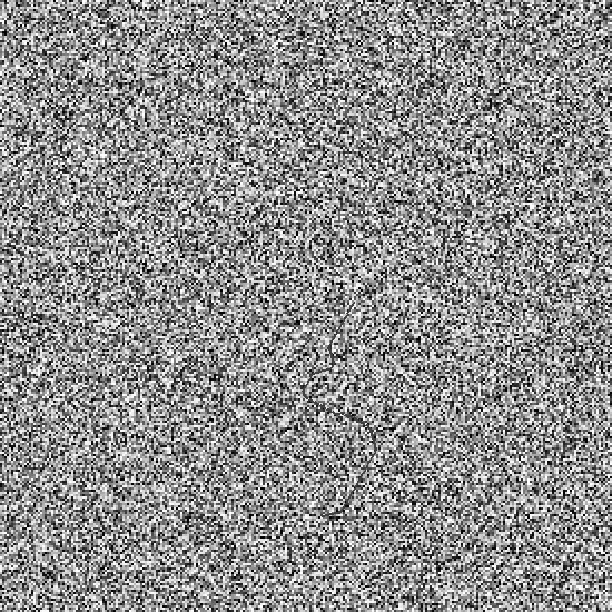
Sample target display at contrast used in the experiments. The target contour is slightly below center.

Figure 2.

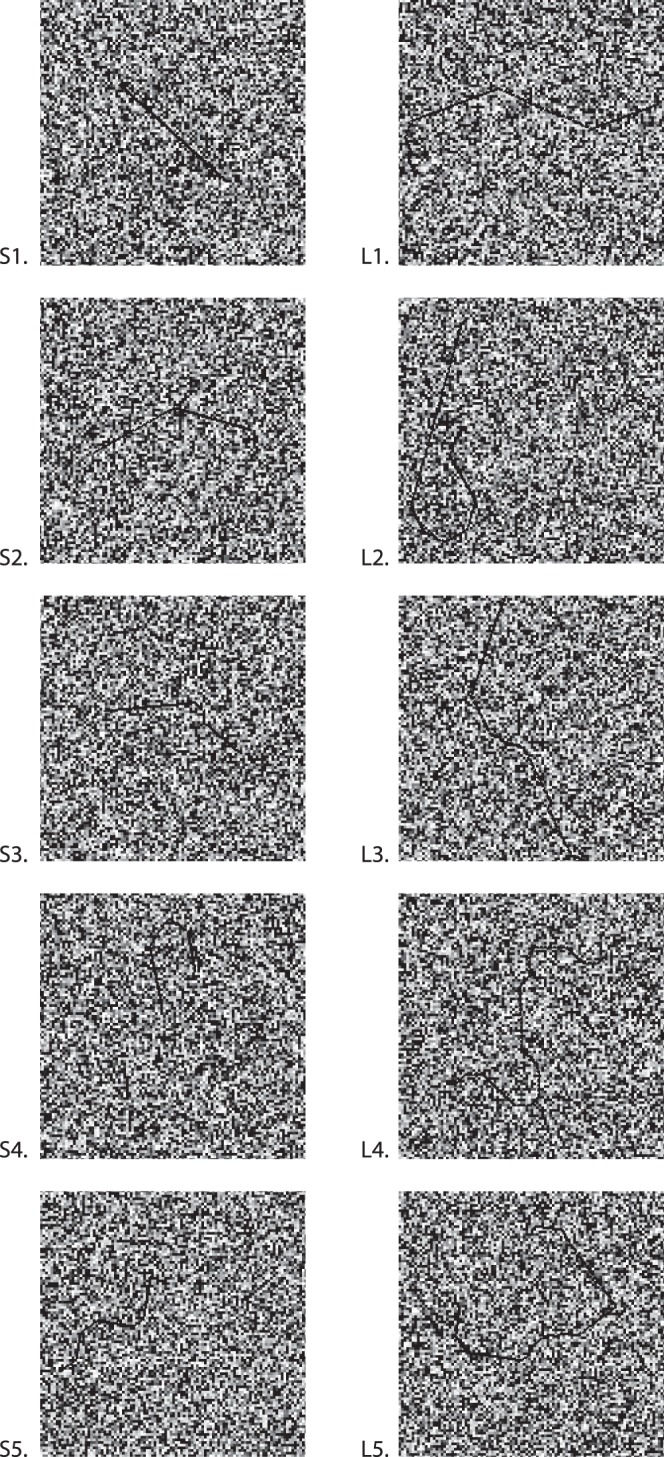
Sample displays containing short contours (left) and long contours (right), showing several levels of complexity (DL). Complexity increases from top to bottom rows. Targets in this figure have augmented contrast compared to the experimental displays.

Figure 3.

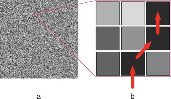
(a) Sample image, with contour target, from experiments. (b) Blowup of a patch of the image, showing a chain of equal luminance pixels. The observer must decide if this path is a smooth path drawn from the von Mises model, or a random walk resulting from the pixel noise.

We begin by deriving a simple model of how an observer can distinguish an image that contains a target generated from the smooth contour model (above) from an image that does not (pure pixel noise). The target curve consists of a chain of dark pixels passing through a field of pixels of random luminances. Contours were set to 64% contrast (measured as the luminance of the contour minus the mean luminance of the image background, divided by the mean luminance of the background). Within each local image patch, a simple strategy to distinguish a target from a distractor is to consider the darkest path through the patch, and decide whether the path is more likely to have been generated by the smooth curve model, C, with von Mises distributed turning angles, or is simply part of a patch of random background pixels (Figure 3), which we will refer to as the “null” model, H₀. We can use Bayes's rule to assess the relative probability of the two models, and then extend the decision to a series of image patches extending the length of the potential contour.

Under the smooth contour model, the observed sequence of turning angles has likelihood given in Equation 4, the product of an i.i.d. sequence of von Mises (or normal) angles. Conversely, under the null model, the contour actually consists of pixel noise, and each direction is equally likely to be the continuation of the path, yielding a uniform distribution over turning angle, p(α|H₀) = ϵ. In our displays, ϵ = 1/3 because the curve could continue left (45°), straight, or right (45°), all with equal probability⁴, but here we state the theory in more general terms. In the null model, as in the contour model, we assume that turning angles are all independent conditioned on the model, so the likelihood of the angle sequence [α_i] is just the product of the individual angle probabilities,

reflecting a sequence of N “accidental” turning angles each with probability ϵ.

By Bayes's rule, the relative probability of the two interpretations, H_C and H₀, is given by the posterior ratio p(C|[α_i]) / p(H₀|[α_i]). Assuming equal priors, which is reasonable in our experiments as targets and distractors appear equally often, this posterior ratio is simply the likelihood ratio, L_C/L₀. As is conventional, we take the logarithm of this ratio to give an additive measure of the evidence in favor of the contour model relative to the null model, which is sometimes called the weight of evidence (WOE):

The first term in this expression, the log likelihood under the contour model, is familiar as the (negative of the) description length (DL), defined in general as the negative logarithm of the probability:

As Shannon (1948) showed, the DL is the length of the representation of a message, M, having probability, p(M), in an optimal code, making it a measure of complexity of the message, M.⁵ Once the coding language is optimized, less probable messages take more bits to express. In our case, plugging in the expression for the likelihood of the contour model (Equation 4), the DL of the contour [α_i] is just

and the weight of evidence in favor of the contour model is

the negative of the DL minus a constant.

For a contour of a given length N, the only term in Equation 8 that depends on the shape of the contour is the sum of the squared turning angles along its length (the N ln ϵ term is a constant that does not depend on the observed turning angles). The larger this sum, the more the contour undulates, and the higher its DL. The larger the DL, the less evidence in favor of the smooth contour model; the smaller the DL, the smoother the contour, and the more evidence in favor of the smooth model.

Hence, the Bayesian model leads directly to a simple prediction about contour detection performance: it should decline as contour DL increases. The larger the DL, the less intrinsically detectable the contour is, and the more the contour is intrinsically indistinguishable from pixel noise. Because this prediction follows so directly from a simple formulation of the decision problem, in what follows we treat it as a central empirical issue. In our experiments, we manipulate the geometry of the target contour, specifically its constituent turning angles, and evaluate observers' detection performance as a function of contour DL. More specifically, our data can be regarded as a test of the specific contour likelihood model we have adopted, which quantifies the probability of each contour under the model and thus, via Shannon's formula, its complexity.

As suggested by Attneave (1954), contour curvature conveys information; the more the contour curves, the more “surprise” under the smooth model, and thus the more information required to encode it (Feldman & Singh, 2005). But DL, Shannon's measure of information, is also a measure of the contour's intrinsic distinguishability from noise. The DL is in fact a sufficient statistic for this decision, meaning that it conveys all the information available to the observer about the contour's likelihood under the smooth contour model.

Of course, as discussed above, it is well known that contour curvature decreases detectability, and the derived dependence on the summed squared turning angles may simply be regarded as one way of quantifying that dependence. But the above derivation substantially broadens this argument because (a) it shows how the specific choice of contour curvature measure, the summed squared angle, derives from a standard contour generating model; and (b) it shows how the predicted decrease in detectability relates to the DL, which is a more fundamental relationship that generalizes far beyond the current situation. From this point of view, contour detection is simply a special case of a more general problem, the detection of structure in noise. Generalizing the argument above, whenever the target class can be formulated as a stochastic generative model with an associated likelihood function, detection performance should decline as DL under the model increases. In the experiments below, we test this prediction for the case of open (nonclosed) contours.

Equations 8 and 9 also predict that longer contours will be more detectable than short ones, because detectability increases with N, the length of the contour (note that ln ϵ in these equations is a negative number because ϵ < e). By itself, this prediction is somewhat less interesting because it would probably follow from any reasonable model so, in what follows, we mostly focus on the complexity effect, which is more specific to our approach. However, it is worth noting that this prediction falls out of our model in a natural way without any ad hoc assumptions about the influence of contour length.

Experiment 1

Method

Subjects

Ten naive subjects participated in the experiment as part of course credit for an introductory psychology course.

Procedure and stimuli

Stimuli were displayed on a gamma-corrected iMac computer running Mac OS X 10.4 and MATLAB 7.5 (MathWorks, Natick, MA), using the Psychophysics toolbox (Brainard, 1997; Pelli, 1997).

The task was a two-interval forced-choice (2IFC) task. The subjects viewed two images, one after the other, and were asked to decide if a contour was present in the first image or the second. Masking images were presented prior to the first target image, between the images, and after the second target image. Presentation time for each stimulus image and each mask image was 500 ms, with 100 ms blank screens in between the first image and the mask and between the mask and the second image. Such long presentation times were required to allow our subjects to successfully carry out the task. Presentation times long enough to allow eye movements obviously complicate the strategies potentially available to subjects, as will be discussed below. However note that many contour detection studies, for example, those of Field et al. (1993), have used long presentation times, without unacceptable complications. All images were presented at about 13° of visual angle. Each image was 15 × 15 cm on the display. The head position was not constrained, but was initially located at 66 cm from the display and subjects were instructed to remain as still as possible. If necessary, during three breaks, which were evenly spaced throughout the experiment, the head was repositioned to be 66 cm from the display.

The target images were created by randomly sampling a 225 × 225 matrix of intensity values. Each pixel intensity was drawn from a uniform distribution between 0 and 98 cd/m². A contour would be embedded in one of two target images. The contour was either a “long” contour (220 pixels, 5.25° if the contour was entirely straight) or a “short” contour (110 pixels, 2.62° if entirely straight). The contour was generated by sampling sequential turning angles (α) using a discretized approximation to a von Mises distribution. Continuing straight (α = 0) is more common than a turning angle right or left (α = π/4 or α = −π/4). Once the contour was generated, it was dilated using the dilation mask [0 1 0;1 1 0;0 0 0], chosen so that a perfectly straight contour oriented horizontally or vertically was detected as easily as one oriented at an arbitrary angle in a pilot study involving author JDW as the observer. Next, to prevent the contour from appearing at a different scale from the random pixels in the image, the image was increased in size to 550 × 550 pixels, using nearest-neighbor interpolation so that each pixel in the smaller image became a 2 × 2 pixel area in the image. Finally, the contour was embedded in one of the target images. The contour was randomly rotated, and then placed at a random location in the image, with the restriction that the contour could not extend beyond the edge of the image.

The masks were random noise images consisting of black (0 cd/m²) and white pixels (98 cd/m²). The images were created by randomly sampling a binary matrix of size 225 × 225, and then scaling the matrix to 550 × 550 using nearest-neighbor interpolation, just as in the target images.

The contours embedded in one of the target images were one of five different complexity levels and one of two lengths (110 pixels or 220 pixels; see Figure 2). Each contour was displayed at 17.5 cd/m², or 64% contrast. Figure 1 shows a sample stimulus at the contrast used in the experiments; stimuli in Figure 2 show enhanced contrast. There were 40 images of each length and each complexity, resulting in a total of 40 × 2 × 5 = 400 trials. The luminance of the contour, image size, and contour lengths were chosen so that, in a pilot study, subjects performed near 75% correct.

Results and discussion

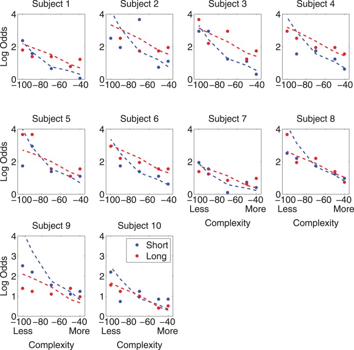
Every subject showed some level of decrease in detection as the complexity of the stimuli increased (see Figure 4); we used log odds of a correct response as a dependent measure to allow valid use of linear regression (see Zhang & Maloney, 2012). Using linear regression, all 20 subjects' slopes (20 out of 20) were negative, suggesting that complexity consistently and significantly affected performance (sign–rank test, p = 1.9 × 10⁻⁶). Five of 10 subjects showed a significant complexity effect (p < 0.05) in the short contour condition, and five of 10 showed a significant effect in the long contour condition. All but two of the subjects showed a significant complexity effect in at least one of the length conditions. In an aggregate analysis (Figure 5), there was a main effect of complexity, F(4, 89) = 18.55, p = 4.07 × 10⁻¹¹, but none of contour length and no interaction at the p = 0.05 level. Looking at contour length in more detail, eight out of 10 subjects showed a superiority for long contours (individually significant in two subjects, p < .05), while two in 10 showed a very small (nonsignificant) superiority for short contours. These results together suggest at best a marginal trend towards the expected effect of contour length. The slope of the best fitting regression line to the combined subjects' data was −0.027 for short contours and −0.02 for long contours.

Figure 4.

Performance (log odds of a correct answer) for each subject in Experiment 1 as a function of contour complexity (DL). Red indicates long contour trials, and blue indicates short contour trials. The dashed lines show the best fitting model. The model contained one free parameter, the standard deviation of the normal distribution, which was sampled to add to the turning angles. For 10 of the 20 fits, the model outperforms (explains more variance than) a one-parameter linear fit.

Figure 5.

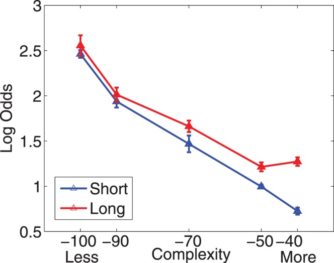
Performance (log odds of a correct answer) in Experiment 1 is shown as a function of the contour complexity (DL) for all of the subjects' data combined. The red points show the detection when subjects' were shown a long contour (220 pixels) and the blue points show a short contour (110 pixels). Error bars show one standard error. For both contour lengths there is a decrease in performance with increasing complexity.

These results show that our subjects are sensitive to the complexity of the target contour's shape, as expected under the Bayesian framework and the assumed generative model. This finding gives strong prima facie support for the Bayesian approach, suggesting that contour detection is an approximately optimal process, given suitable assumptions about the stochastic structure of smooth contours.

Cocircularity

As an additional analysis, we next ask whether our subjects' performance shows any influence of contour cocircularity (minimization of change in turning angle), which has also been found to play a role in the perception of contour smoothness (Feldman, 1997; Motoyoshi & Kingdom, 2010; Parent & Zucker, 1989; Pettet, 1999). As suggested in Singh & Feldman (2013), our probabilistic contour model can easily be extended to by adding a distribution over the “next higher derivative” of the contour tangent. Turning angle α is a discretization of the derivative of the tangent with respect to arclength (i.e., curvature), and change in turning angle Δα is a discretization of the second derivative of the tangent with respect to arclength (i.e., change in curvature). To incorporate this, we simply assume that, Δα (just like α itself) is von Mises distributed,

where β_Δ is a suitably chosen spread parameter. Under the “basic” von Mises model, turning angles were i.i.d., but under the augmented model, successive angles are biased to have similar values, with probability decreasing with deviation from cocircularity, as well as with increasing turning angle itself as before. As before, this von Mises distribution is very closely approximated by a Gaussian centered at 0°, meaning that, in the augmented model, the joint likelihood p(α, Δα|H_C) is well approximated by a bivariate Gaussian centered at (0°, 0°).

With this augmented model in hand, we then quantify the complexity of a contour [α_i] exactly as before, as −log(p([α_i]) summed along the contour. The new DL measure penalizes contours that deviate from circularity in addition to deviation from straightness, meaning that contours are penalized not only when they bend but when the degree of bend changes.

Unfortunately, our study as constructed is not ideal for evaluating the empirical effect of this DL measure because the turning angles in the target contours were generated i.i.d. (levels of cocircularity are random, so very cocircular contours are relatively rare). Moreover, α and Δα are not independent (r = .83), meaning that the influence of DL due to change in turning angle is confounded with the DL due to turning angle itself. Nevertheless, as a reasonable post hoc analysis, we can compare the DL due to the original model with the augmented DL incorporating the cocircularity bias. This analysis yields mixed results. Using a linear regression onto log odds, we find that the added factor of Δα DL provides a significantly better fit to the data than the turning angle DL by itself (by a chi-square test of fit with nested models) in the case of short contours (p = 0.033), but only marginally significant in the case of long contours (p = 0.084). This suggests, consistent with previous literature, that contour cocircularity plays a measurable role in the detection of smooth contours, albeit a smaller one than collinearity itself. We emphasize, however, that this result should be interpreted with caution because of the high correlation between smoothness factors inherent in the design of the experiment.

We were concerned with several potential confounds. First, one might wonder if lower-complexity contours occupy larger visual areas, because, by definition, they follow straighter paths. If so, an observer searching through the image (either attentionally or via overt eye movements, which our presentation times are long enough to allow) would be more likely to happen upon lower-complexity contours than higher complexity ones. However, a simple analysis shows that this concern is unfounded. We computed the spatial density of target contour pixels in the stimuli, which indicates where in the displays a search strategy would be more likely to encounter a target. Figure 6 shows target pixel density in the stimulus displays as a function of eccentricity, separately for all levels of contour complexity and contour length. Because targets were not allowed to fall off the edge of the display, necessitating some concentration near the center, target pixel density decreases with eccentricity in all the plots, meaning that targets were generally located near fixation. Critically, however, the fall-off with eccentricity is approximately the same for all levels of complexity (columns in the figure). That is, the spatial distribution of targets is unrelated to contour complexity, so such a search strategy cannot explain the complexity effect we found.

Figure 6.

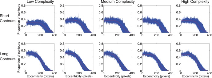
Density of target contour pixels, plotted for short and long contours (top and bottom rows, respectively) and all levels of contour complexity (columns, increasing in complexity from left to right). Target density decreases sigmoidally with eccentricity, but does so approximately equivalently for all conditions, meaning that complexity is not confounded with target complexity. That is, although searching near fixation was an effective strategy (subjects were asked to fixate but eye movements were not controlled), such a strategy was no more or less likely to be effective at low levels of contour complexity than at high levels.

Conversely, one might wonder if our effect could be explained by a strategy of searching for regions of distinct luminance because, by design, target contours have a different mean luminance than background textures. However, if high-complexity contours are more tightly “curled” than low-complexity contours, they would correspond to more concentrated regions of distinct luminance. Of course, the complexity effect goes in the other direction, with lower-complexity contours being easier on average to find so, again, this tendency (which is apparently negligible in any case, given Figure 6) could not explain the observed complexity effect.

Finally, we were concerned that a strategy of simply searching for long, straight segments might explain our subjects' performance. If so, our complexity measure, which reflects the geometry of the entire contour, would be unwarranted. We designed Experiment 2 to check this possibility.

Experiment 2

The complexity measure used in Experiment 1 assumes integration along the entire contour, but it is possible that the detectability of a contour is only based on the local complexity at an individual contour point. That is, the results from the first experiment might be explained by a model of detection that simply looks for straight segments, rather than evaluating the geometry of the entire contour. If so, the complexity effect could be due simply to the fact that simple (low DL) contours tend to have long straight segments. To evaluate this alternative hypothesis, in Experiment 2 we manipulated the spatial distribution of the complexity, concentrating a large majority (90%) of the curvature in either the second eleventh (the tip), fourth eleventh (between the tip and the middle), or sixth eleventh (the middle) of the contour. This manipulation effectively modulates the length of the longest straight segment while holding complexity (DL) approximately constant. Contours with the bending concentrated at the tip, for example, will have relatively long straight segments, while having on average no higher or lower complexity than those with the bend concentrated in the middle. The aim of the experiment is to determine whether this factor, rather than DL itself, modulates performance.

Method

Subjects

Ten naive subjects participated for course credit as part of an introductory psychology course. The data of two subjects were excluded because they were at chance performance for all conditions. Exit interviews suggested that these subjects did not understand the task.

Procedure and stimuli

Each trial was conducted in the same manner as Experiment 1. The only difference in the stimulus was that the location of 90% of the surprisal was controlled to be at the second eleventh of the contour (the tip), the fourth eleventh of the contour (between the tip and the middle, or the sixth eleventh of the contour (the middle). There were 396 trials (four different surprisals and three locations, with 33 trials per crossed conditions).

Results and discussion

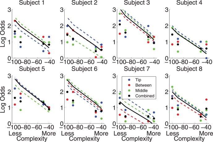
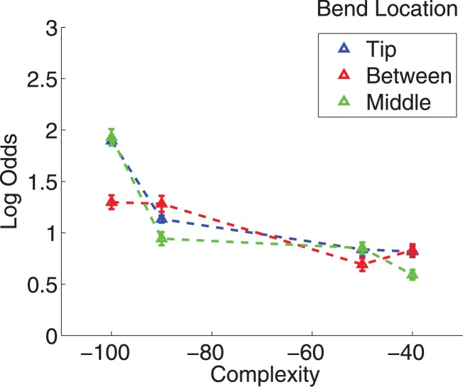
Complexity decreased detectability, just as in Experiment 1, in all conditions for all but one subject (Figure 7). Combining subject data (Figure 8) shows a significant main effect of complexity, F(3, 42) = 18.99, p = 6.18 × 10⁻⁸, and no main effect of bend location, F(2, 42) = 0.94, p = 0.397.

Figure 7.

Performance (log odds of a correct answer) of each subject in Experiment 2 as a function of the contour complexity (DL). The colors denote the different bend location conditions: blue for bend at the tip, red for bend between the middle and the tip, green for the bend at the middle of the contour, and black for average across conditions. Dashed lines show the best fitting models for each condition, and the solid line is the fit for the model fit with the constraint that the model parameter must be the same for all three locations. The decrease in detectability as complexity increased found in Experiment 1 was found in all conditions.

Figure 8.

Performance (log odds of a correct answer) in Experiment 2 as a function of the contour complexity (DL) for the subjects' combined data. As seen in Experiment 1, performance decreases with complexity (DL). There is no apparent difference between the different bend locations.

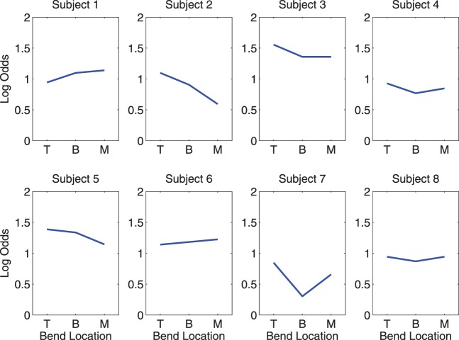
The manipulation of the location of the complexity in the contour can be seen to have had no consistent effect for the individual subjects when looking at percent correct versus the bend location (Figure 9). Combining subjects' data (Figure 10) also shows no trend. That is, the failure of the ANOVA to find a significant main effect of bend location was not a result of finding a weak trend in the correct direction with too little data to find significance, but rather reflects the absence of a trend in the direction predicted by an account based only on straight segment detection.

Figure 9.

For each subject, the performance (log odds of a correct answer) in Experiment 2 is shown as a function of the bend location (location of the majority of the curvature). The different bend locations are denoted by “T” (tip), “B” (between the tip and middle), and “M” (middle). There was no consistent decrease in detectability as the location was varied.

Figure 10.

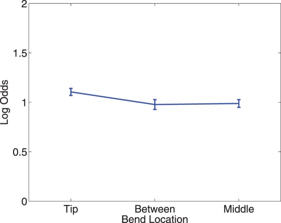
Performance (log odds of a correct answer) as a function of the location of contour complexity (DL) for all of the subjects' data from Experiment 2 combined. There appears to be no effect of the location of the complexity.

These data suggest that the effect of complexity found in Experiment 1, and replicated in Experiment 2, is not due solely to the spatial distribution of the complexity throughout the contour. Humans are not simply straight segment detectors; the complexity of the entire contour, as reflected in its integrated description length, influences the detectability of the contour. This finding is consistent with previous work arguing for the importance of nonlocal information in shape and contour representation (Feldman et al., 2013; Singh, in press; Wilder, Feldman, & Singh, 2011).

General discussion

Contour curvature is well known to influence human detection of contours (Field et al., 1993; Field et al., 2000; Geisler et al., 2001; Hess & Field, 1995, 1999; Pettet et al., 1998; Yuille et al., 2004). Exactly why curvature has this effect is still poorly understood, however, as reflected in the lack of mathematical models that can adequately capture it. In this paper we have modeled contour detection as a statistical decision problem, showing that a few simple assumptions about the statistical properties of smooth contours make fairly strong predictions about the performance of a rational contour detection mechanism, specifically that its performance will be impaired by contour complexity. Contour complexity, in turn, involves contour curvature as a critical term (the only term that reflects the shape of the contour), thus giving a concrete quantification of the effects of contour curvature on detection performance. The data strongly corroborate the effect of complexity on contour detection, showing strong complexity effects in almost every subject. Moreover, the spatial distribution of the complexity does not seem to determine performance, suggesting that a purely local complexity measure (such as the information/complexity defined at each contour point) will not suffice to explain performance, and a holistic measure of contour complexity (such as contour description length) is required.

Our results are not predicted by many of the standard object detection algorithms used in computer vision; indeed, many of these models are unable to locate the objects in our displays at all. Many of the standard edge detection algorithms rely on finding strong luminance discontinuities in the image. For example, the Marr-Hildreth algorithm uses Laplacian of Gaussian (LOG) filters, due to their similarity to response properties of cells in lateral geniculate nucleus (LGN) (Marr & Hildreth, 1980). These filters fail to increase their responses near the contours in both experiments because the filters need a difference between the luminance in the center from the luminance in the surround. In our stimuli there is noise everywhere and our contours have the same luminance as many pixels that are actually part of the noise. Other edge detection algorithms, such as the Canny edge detector, the Hough Transform, and the Burns line finder also look for high magnitude image gradients, which are not present in our images (Burns, Hanson, & Riseman, 1986; Canny, 1986; Duda & Hart, 1972; Hough, 1962). Also, these methods frequently smooth the input image prior to detecting edges, which, with our images, would simply cause the contour to blend further into the noise and thus substantially weaken image gradients.

Edges in images result in a strong component in the power spectrum perpendicular to the edge in the image. One possible explanation for our effect is that the power spectrum of images containing straighter contours is more distinguishable from the power spectrum of noise images than the power spectrum in images with curved contours. This turns out not to be the case. The power spectrum of the images used in the experiments reveals that there is energy at all frequencies, not just predominantly at low spatial frequencies as is common in natural images. This suggests that the reason standard edge-detection algorithms are unable to detect the contours is because our images are of a different structure than that present in the natural images for which these algorithms were developed. However, our subjects were able to accurately detect the contours, suggesting that the human visual system is doing something different than these algorithms.

If standard computer vision algorithms fail to detect contours, perhaps a more optimal observer, with full access to the pixel content of the image, would be able to detect the contours and better explain our subjects' behavior. A more detailed consideration of the statistical decision problem suggests that our observers are far from optimal. To see why, consider the contour detection problem reduced to a simple Bernoulli problem. The target contour consists of a series of turns through the pixel grid, each of which can be classified as either a straight continuation (a success or “head”) or a nonstraight turn (a failure or “tail”). Smooth contours have a strong bias toward straight continuations (successes), translating to a high success probability, the exact value of which depends on the spread parameter β in the von Mises distribution that generates the turning angles (see Equation 10), which in turn depends on the condition. In contrast, each distractor path consists of a series of random turns in which the probability of straight continuation is ϵ (1/3, as explained above; see Figure 3). The observer's goal is to determine, based on the sample of turns observed, whether the sample was generated from the smooth process (i.e., a target display) or the null process (distractor display). Because successive turning angles are assumed independent, this means that a smooth curve consists, in effect, of a sample of N (219 or 109 on long and short trials, respectively) draws from a Bernoulli process with high success probability (which varies by condition but is often very high, > 0.9), while noise consists of a sample with success probability 1/3.

To make a decision in these experiments, the observer must consider the number of straight continuations observed in the smoothest contour in each display, and decide which stimulus interval was more likely to contain a sample generated by a process with high success probability (again, with the level dependent on condition). This is a standard Bernoulli Bayesian decision problem, specifically a forced choice version (see for example, Lee, 2004). Because the two success probabilities (0.9 vs. 0.33) are so different and the sample size is so large (209 or 109), this is actually an easy decision; an optimal observer with full information about the pixel content of the images in both intervals is at ceiling in all conditions, since in even the highest DL conditions the success probability is much higher than 1/3. In other words, if the observer had access to the full pixel content of each image it would integrate the contour on every trial. A decision procedure that simply chooses the image containing the longest of the candidate contours would perform perfectly, with no effect of complexity.

Obviously, our observers do not have full access to the pixel content of both images, which contain far more information than can be fully acquired under our speeded and masked experimental conditions. A variety of simple assumptions can be made about how image information is limited or degraded, but most give predictions that differ in various ways from what we observed. For example, one might assume that subjects only apprehend a part of the target contour, rather than the contour in its entirety; this predicts subceiling performance, but also predicts a much smaller complexity effect than is actually observed. In any case, the results of Experiment 2 strongly suggest that observers are sensitive to the complexity of the entire contour, not just to short segments of it. Similarly, one can imagine various search strategies that observers might adopt, which would modulate the probability that the target contour is encountered, but as explained above, such strategies cannot explain the effect of contour complexity.

We did, however, find one simple set of assumptions about information degradation that fit our data well. It is reasonable to assume that turning angles, rather than being encoded perfectly as the ideal model assumes, are degraded via the addition of angular noise. We constructed a model in which turning angles, instead of being 0 or ±45° (as they are in the displays) were respectively 0 + N(0,σ²) or ±45° + 0 + N(0,σ²) where the standard deviation σ is a parameter fit to each observer. This simple one-parameter model provides a good fit our subjects' data (Figure 4), including both the absolute level of performance and the magnitude of the complexity effect. All subjects' model fits were fairly similar, with a mean σ = 24.45° and standard deviation of 0.35° in the short contour condition, and a mean σ = 25.06° and standard deviation of 0.41° in the long contour condition. This model accommodates the complexity effect predicted by the original classification model, while also reflecting, in a particularly simple way, the stimulus uncertainty present in the real visual system.

Additionally, we found further support, using the data in Experiment 2, that the total complexity of each contour is more important than the way it is spatially subdivided within each contour. We fit the noise model to our subjects' data and either let the σ parameter vary separately for the three conditions (tip, between, or middle) or we constrained σ to be the same in all of these conditions. Using the likelihood ratio test we found that the additional model complexity involved in letting σ vary for each condition was not justified for any of our subjects, suggesting that subjects were sensitive to contour complexity in approximately the same way throughout the entire contour. The likelihood ratio test compares the likelihood of a model with with multiple parameters to a nested model with fewer parameters to see if the inclusion of these additional parameters is justified. Specifically it computes

where C is the constrained version of the model (in our case, a one-parameter model), U is the unconstrained model (in our case, the three-parameter model in which each bend location has its own angle noise parameter), and Λ is

and

where M is a model (either constrained or unconstrained), n = 12 is the number of conditions (one for each contour complexity crossed with each bend location) P_m is the proportion correct for a condition, and P_s is the subject performance in that condition.

The constrained model can explain then subject performance in the different conditions as well as a model that allows for each bend location to be fit separately. The likelihood-ratio test statistics ranged from 0–0.54, with a mean of 0.36 and standard deviation of 0.19. The likelihood-ratio test statistics are distributed as a χ² distribution with degrees of freedom equal to the difference in the number of parameters of the models (in our case 2). This results in p values ranging from 0.76–1, with a mean of 0.84 and standard deviation of 0.08. The quality of the fits in the constrained model were not significantly worse than the fits in the unconstrained model, so we are not justified in using a model that treats the bend locations differently. The constrained model had similar parameters to the fits in Experiment 1, a mean σ = 24.88°, and standard deviation of 0.33°.

In summary, our subjects' performance can be accounted by a Bayesian observer model that assumes turning angles are noisily encoded by the visual system. This model encodes the complexity of the contour as a whole, and the spatial distribution of the complexity does not affect performance.

Conclusion

Here we have framed the contour detection problem as a Bayesian inference problem. We defined a simple generative model for contours, in which successive turning angles are generated from a straight-centered distribution. The observer's task then reduces to a probabilistic inference problem in which the goal is to decide which of the two stimulus images was more likely to contain a contour sample drawn from this generative model. This framing of the problem accounts for key aspects of the empirical results, in particular the influence of contour complexity on detection. Although our subjects may well have carried out search strategy of some kind (as in any difficult detection task with long presentation times), such a strategy cannot explain the effect of contour complexity. We also found that the spatial distribution of complexity appears not to matter substantially; the deciding factor is the smoothness of the entire target taken as a whole. Both of these results go beyond standard accounts of contour integration (Field et al., 1993; Geisler et al., 2001; Geisler & Super, 2000), especially in the quantitative precision with which they can account for the influence of contour structure. Additionally, our modeling suggests that subjects' encoding of stimulus turning angles is noisy, depressing their performance relative to an ideal observer in possession of perfect image data.

Fundamentally, the Bayesian model described here makes it clear why a diminution in performance as curvature increases “makes sense”—it is a direct consequence of a very general contour model and a rational contour classification mechanism. As argued in the Introduction, the problem of contour detection is really just a special case of the more general problem of the detection of pattern structure in noise. As shown above, a very general model of the probabilistic detection of regular structure in noise entails an influence of target complexity, defined from an information-theoretic point of view as the negative log of the stimulus probability under the generative model, that is the Shannon complexity or description length (DL) of the pattern. The ubiquitous influence of simplicity biases and complexity effects in perception and cognition more generally can be seen as a consequence of the general tendency for simple patterns to be more readily distinguishable from noise (Chater, 2000; Feldman, 2000) than complex ones (Feldman, 2004). In past studies, contour detection has usually been studied as a special problem unto itself whose properties derived from characteristics of visual cortex. Instead, we hope that in the future the problem of contour detection can be treated as a special case of a broader class of pattern detection problems, all of which can be studied in a common mathematical framework in which they differ only in details of the relevant generative models (Feldman, Singh, & Froyen, in press). This observation opens the door to a much broader investigation of perceptual detection problems encompassing detection of patterns and processes well beyond simple contours, such as closed contours and whole objects.

References

- Attneave, F.(1954). Some informational aspects of visual perception. Psychological Review, 61(3), 183–193. [DOI] [PubMed] [Google Scholar]
- Brainard D.(1997). The Psychophysics Toolbox. Spatial Vision, 10, 433–436. [PubMed] [Google Scholar]
- Burns J. B.,, Hanson A. R.,, Riseman E. M.(1986). Extracting straight lines. IEEE Transactions on Pattern Analysis and Machine Intelligence, 8(4), 425–455. [Google Scholar]
- Canny J.(1986). A computational approach to edge detection. IEEE Transactions on Pattern Analysis and Machine Intelligence, 8(6), 679–698. [PubMed] [Google Scholar]
- Chater N.(2000). Cognitive science: The logic of human learning. Nature, 407, 572–573. [DOI] [PubMed] [Google Scholar]
- Duda R. O.,, Hart P. E.(1972). Use of the Hough transformation to detect lines and curves in pictures. Commununications of the ACM, 15, 11–15. [Google Scholar]
- Elder J.,, Goldberg R.(2002). Ecological statistics of Gestalt laws for the perceptual organization of contours. Journal of Vision , 2(4): 5, 324–353, http://www.journalofvision.org/content/2/4/5, doi: 10.1167/2.4.5. [PubMed] [Article] [DOI] [PubMed] [Google Scholar]
- Ernst U. A.,, Mandon S.,, Schinkel-Bielefeld N.,, Neitzel S. D.,, Kreiter A. K.,, Pawelzik K. R.(2012). Optimality of human contour integration. PLoS Computational Biology, 8(5), e1002520. [DOI] [PMC free article] [PubMed] [Google Scholar]
- Feldman J.(2001). Bayesian contour integration. Perception & Psychophysics, 63(7), 1171–1182. [DOI] [PubMed] [Google Scholar]
- Feldman J.(1995). Perceptual models of small dot clusters. Cox I. J., Hansen P., Julesz B.(Eds.)Partitioning data sets (Vol. 19, 331–357) Providence, RI: American Mathematical Society. [Google Scholar]
- Feldman, J.(1997). Curvilinearity, covariance, and regularity in perceptual groups. Vision Research, 37, 2835–2848. [DOI] [PubMed] [Google Scholar]
- Feldman J.(2000). Minimization of Boolean complexity in human concept learning. Nature, 407, 630–633. [DOI] [PubMed] [Google Scholar]
- Feldman J.(2004). How surprising is a simple pattern? Quantifying “Eureka!” Cognition, 93, 199–224. [DOI] [PubMed] [Google Scholar]
- Feldman J.,, Singh M.(2005). Information along contours and object boundaries. Psychological Review, 112, 243–252. [DOI] [PubMed] [Google Scholar]
- Feldman J.,, Singh M.,, Briscoe E.,, Froyen V.,, Kim S.,, Wilder J.(2013). An intergrated Bayesian approach to shape representation and perceptual organization. Dickinson S., Pizlo Z.(Eds.)Shape perception in human and computer vision: An interdisciplinary perspective (pp 55–70) New York: Springer Verlag. [Google Scholar]
- Feldman, J.,, Singh M.,, Froyen V.(in press). Perceptual grouping as Bayesian mixture estimation. Gepshtein S., Maloney L., Singh M.(Eds.)Oxford handbook of computational perceptual organization. Oxford, UK: Oxford University Press. [Google Scholar]
- Field, D.(1987). Relations between the statistics of natural images and the response properties of cortical cells. Journal of the Optical Society of America, 4, 2379–2394. [DOI] [PubMed] [Google Scholar]
- Field D.,, Hayes A.,, Hess R.(1993). Contour integration by the human visual system: Evidence for a “local association field.” Vision Research, 33, 173–193. [DOI] [PubMed] [Google Scholar]
- Field D.,, Hayes A.,, Hess R.(2000). The roles of polarity and symmetry in the perceptual grouping of contour fragments. Spatial Vision, 13, 51–66. [DOI] [PubMed] [Google Scholar]
- Geisler W.,, Perry J. S.,, Super B.,, Gallogly D. P.(2001). Edge co-occurrence in natural images predicts contour grouping performance. Vision Research, 41, 711–724. [DOI] [PubMed] [Google Scholar]
- Geisler W.,, Super B.(2000). Perceptual organization of two-dimensional patterns. Psychological Review, 107, 677–708. [DOI] [PubMed] [Google Scholar]
- Hess R.,, Field D.(1995). Contour integration across depth. Vision Research, 35, 1699–1711. [DOI] [PubMed] [Google Scholar]
- Hess R.,, Field D.(1999). Integration of contours: New insights. Trends in Cognitive Sciences, 3, 480–486. [DOI] [PubMed] [Google Scholar]
- Hess R.,, Hayes A.,, Field D.(2003). Contour integration and cortical processing. Journal of Physiology–Paris, 97, 105–119 doi:http://dx.doi.org/10.1016/j.jphysparis.2003.09.013. [DOI] [PubMed] [Google Scholar]
- Hough P.(1962). Method and means for recognizing complex patterns. U.S. Patent No. 3,069,654. Washington, DC: U.S. Patent and Trademark Office. [Google Scholar]
- Jaynes E. T.(1988). The relation of Bayesian and maximum entropy methods. Erickson G. J., Smith C. R.(Eds.)Maximum-entropy and Bayesian methods in science and engineering (pp 25–29) Dordrecht, The Netherlands: Kluwer Academic. [Google Scholar]
- Kovacs, I.,, Julesz B.(1993). A closed curve is much more than an incomplete one: Effect of closure in figure–ground segmentation. Proceedings of the National Academy of Sciences, USA, 90, 7495–7497. [DOI] [PMC free article] [PubMed] [Google Scholar]
- Kovács I.,, Polat U.,, Pennefather P. M.,, Chandna A.,, Norcia A. M.(2000). A new test of contour integration deficits in patients with a history of disrupted binocular experience during visual development. Vision Research, 40, 1775–1783 Retrieved from http://www.sciencedirect.com/science/article/pii/S0042698900000080, doi: http://dx.doi.org/10.1016/S0042-6989(00)00008-0. [DOI] [PubMed] [Google Scholar]
- Lee P. M.(2004). Bayesian statistics: An introduction (Third ed.). West Sussex, UK: Wiley. [Google Scholar]
- Li W.,, Gilbert C. D.(2002). Global contour saliency and local colinear interactions. Journal of Neurophysiology, 88, 2846–2856 doi:http://dx.doi.org/10.1152/jn.00289.2002. [DOI] [PubMed] [Google Scholar]
- Marr D.,, Hildreth E.(1980). Theory of edge detection. Proceedings of the Royal Society of London Series B. Biological Sciences, 207(1167), 187–217. [DOI] [PubMed] [Google Scholar]
- Motoyoshi I.,, Kingdom F. A.(2010). The role of co-circularity of local elements in texture perception. Journal of Vision, 10(1): 61–8, http://www.journalofvision.org/content/10/1/3, doi: 10.1167/10.1.3. [PubMed] [Article] [DOI] [PubMed] [Google Scholar]
- Parent P.,, Zucker S. W.(1989). Trace inference, curvature consistency, and curve detection. IEEE Transactions on Pattern Analysis & Machine Intelligence, 11, 823–839. [Google Scholar]
- Pelli D.(1997). The VideoToolbox software for visual psychophysics: Transforming numbers into movies. Spatial Vision, 10, 437–442. [PubMed] [Google Scholar]
- Pettet M. W.(1999). Shape and contour detection. Vision Research, 39, 551–557. [DOI] [PubMed] [Google Scholar]
- Pettet M. W.,, McKee S. P.,, Grzywacz N. M.(1998). Constraints on long range interactions mediating contour detection. Vision Research, 38, 865–879. [DOI] [PubMed] [Google Scholar]
- Ren X.,, Malik J.(2002). A probabilistic multi-scale model for contour completion based on image statistics. Heyden A., Sparr G., Nielsen M., Johansen P.(Eds.)Computer vision–ECCV 2002. ( Vol 2350, 312–327). Berlin, Germany: Springer Verlag. [Google Scholar]
- Sassi, M.,, Vancleef K.,, Machilsen B.,, Panis S.,, Wagemans J.(2010). Identification of everyday objects on the basis of Gaborized outline versions. i-Perception, 1, 121–142 doi:http://dx.doi.org/10.1068/i0384. [DOI] [PMC free article] [PubMed] [Google Scholar]
- Shannon C. E.(1948). A mathematical theory of communication. Bell System Technical Journal, 27, 379–423, 623–656. [Google Scholar]
- Singh M.(in press). Visual representation of contour and shape. Wagemans J.(Ed.)Oxford handbook of perceptual organization. Oxford, UK: Oxford University Press. [Google Scholar]
- Singh, M.,, Feldman J.(2013). Principles of contour information: A response to Lim and Leek (2012). Psychological Review, 119, 678–683. [DOI] [PMC free article] [PubMed] [Google Scholar]
- Singh M.,, Fulvio J. M.(2005). Visual extrapolation of contour geometry. Proceedings of the National Academy of Sciences, USA, 102, 939–944. [DOI] [PMC free article] [PubMed] [Google Scholar]
- Singh M.,, Fulvio J. M.(2007). Bayesian contour extrapolation: Geometric determinants of good continuation. Vision Research, 47, 783–798. [DOI] [PubMed] [Google Scholar]
- Wilder J.,, Feldman J.,, Singh M.(2011). Superordinate shape classification using natural shape statistics. Cognition, 119, 325–340. [DOI] [PMC free article] [PubMed] [Google Scholar]
- Yuille A. L.,, Fang F.,, Schrater P. R.,, Kersten D.(2004). Human and ideal observers for detecting image curves. Thrun S., Saul, L. K., Schökopf (Eds.)Neural information processing systems 16 (NIPS 2003). Cambridge, MA: MIT Press. [Google Scholar]
- Zhang, H.,, Maloney L. T.(2012). Ubiquitous log odds: A common representation of probability and frequency distortion in perception, action, and cognition. Frontiers in Neuroscience, 6, 1. [DOI] [PMC free article] [PubMed] [Google Scholar]
Associated Data
This section collects any data citations, data availability statements, or supplementary materials included in this article.