

Abstract
We model the spread of an (Susceptible Infectious) sexually transmitted infection on a dynamic homosexual network. The network consists of individuals with a dynamically varying number of partners. There is demographic turnover due to individuals entering the population at a constant rate and leaving the population after an exponentially distributed time. Infection is transmitted in partnerships between susceptible and infected individuals. We assume that the state of an individual in this structured population is specified by its disease status and its numbers of susceptible and infected partners. Therefore the state of an individual changes through partnership dynamics and transmission of infection. We assume that an individual has precisely ‘sites’ at which a partner can be bound, all of which behave independently from one another as far as forming and dissolving partnerships are concerned. The population level dynamics of partnerships and disease transmission can be described by a set of differential equations. We characterize the basic reproduction ratio using the next-generation-matrix method. Using the interpretation of we show that we can reduce the number of states-at-infection to only considering three states-at-infection. This means that the stability analysis of the disease-free steady state of an -dimensional system is reduced to determining the dominant eigenvalue of a matrix. We then show that a further reduction to a matrix is possible where all matrix entries are in explicit form. This implies that an explicit expression for can be found for every value of .
Keywords: -infection, Mean field at distance one, Dynamic network, Concurrency,
Introduction
The role that concurrent partnerships might play in the spread of HIV in sub-Saharan Africa is the subject of an ongoing debate. While simulation studies have shown the large impact that concurrency potentially has on the epidemic growth rate and the endemic prevalence of HIV (Kretzschmar and Morris 1996; Morris and Kretzschmar 1997, 2000; Eaton et al. 2011; Goodreau 2011), the empirical evidence for such a relationship is inconclusive (Lurie and Rosenthal 2010; Reniers and Watkins 2010; Tanser et al. 2011; Kenyon and Colebunders 2012).
Mathematical modelling results have played a key role in fuelling the debate (Watts and May 1992; Kretzschmar and Morris 1996; Morris and Kretzschmar 1997, 2000; Eaton et al. 2011; Goodreau 2011). However, a mathematical framework suitable to derive analytical results is still lacking. At present, simulation studies prevail, and general theory is mainly focused on static networks (Diekmann et al. 1998; Ball and Neal 2008; House and Keeling 2011; Lindquist et al. 2011; Miller et al. 2012; Miller and Volz 2013). This motivated us to develop and analyse a mathematical model for the spread of an (Susceptible–Infectious) infection along a dynamic network.
In a previous paper (Leung et al. 2012) a model for a dynamic sexual network of a homosexual population is presented that incorporates demographic turnover and allows for individuals to have multiple partners at the same time, with the number of partners varying over time. This network model can be seen as a generalization of the pair formation models (that describe sequentially monogamous populations) to situations where individuals are allowed more than one partner at a time. Pair formation models were first introduced into epidemiology by Dietz and Hadeler (1988) and extended in various ways (Kretzschmar et al. 1994; Inaba 1997; Kretzschmar and Dietz 1998; Xiridou et al. 2003; Heijne et al. 2011; Powers et al. 2011). In the present generalization, individuals have at most partners at a time. We call the partnership capacity. In the partnership network individuals are, essentially, collections of ‘binding sites’ where binding sites can be either ‘free’ or ‘occupied’ (by a partner). In the case that we recover the pair formation model of a monogamous population.
Consider an individual in the sexual network. Since individuals may have several partners simultaneously, the risk of acquiring infection depends on that individual’s partners, but also on their partners, and so on. We would need to keep track of the entire network to fully characterize the risk of infection to an individual. Here we introduce an approximation rather than taking full network information into account: we assume that properties concerning partners of partners can be obtained by averaging over the population. This approximation is termed the ‘mean field at distance one’ assumption (‘mean field at distance one’ should be read as one term; from here on we write this without quotation marks). This assumption relates to what is called ‘effective degree’ in Lindquist et al. (2011), where transmission of infection along a static network is studied (we are, apart from Britton and Lindholm 2010; Britton et al. 2011), not aware of any analytical work so far, on disease transmission across dynamic networks with demography (see e.g. Altmann 1995, 1998; Ferguson and Garnett 2000; Bansal et al. 2010; Kiss et al. 2012; Miller and Volz 2013) and references therein for models incorporating dynamic partnerships in a demographically closed population).
The mean field at distance one assumption is a moment closure approximation obtained by ignoring certain correlations between the states of two individuals that are in a partnership and, as a consequence, this assumption is inconsistent with the assumptions that underlie the partnership network (see e.g. Ferguson and Garnett 2000; Kamp 2010; House and Keeling 2011; Taylor et al. 2012) and references therein for different moment closure approximations on networks). However, this assumption allows us to write down a closed system of ODEs to describe an approximation of the infection on the partnership network. If a partnership capacity is given, then we have an dimensional system of ODEs.
A large part of the paper is devoted to characterizing the basic reproduction number and proving its threshold character for the nonlinear system of ODEs. This system is quite large already for small . However, by considering only states-at-infection and using the next-generation matrix approach, can be characterized as the dominant eigenvalue of an matrix. Using the interpretation we can further reduce this and can ultimately be characterized as the dominant eigenvalue of a matrix where the entries of this matrix are explicit, and therefore also has an explicit expression. In fact, we are able to interpret in terms of individuals (which are considered in the model specification) and in terms of binding sites.
The structure of the paper is as follows. First, in Sect. 2, we consider the partnership network of Leung et al. (2012) and summarize the main results needed for this paper. Next, in Sect. 3 we superimpose an -infection on the network and specify the model assumptions. Particular attention is given to the mean field at distance one assumption. The rest of the paper is devoted to characterizing the basic reproduction number . For this, in Sect. 4, we first consider the linearisation of the system.
In Sect. 5, which constitutes the core of the paper, we characterize in terms of newly infected binding sites that produce newly infected binding sites. We introduce a transition matrix and a transmission matrix and define as the dominant eigenvalue of the next generation matrix (Diekmann et al. 2013, Section 7.2). The building blocks for an explicit expression for are presented in Appendix C. We also show that thus defined can be interpreted as the basic reproduction ratio for individuals, since individuals can be considered to be collections of binding sites. Section 5 can be read independently of the rest of the paper.
The characterization of in Sect. 5 does not, by itself, provide a mathematical proof that the disease-free steady state is stable for and unstable for . We provide such a proof in Sect. 6. The proof is based on the Perron–Frobenius theory of spectral properties of positive and positive-off-diagonal irreducible matrices. In particular we use that
where is the Malthusian parameter (i.e. the dominant eigenvalue) of the matrix
the linearised system derived in Sect. 4 can be mapped in a natural way to the binding-site system defined by the matrices and , while preserving positivity.
The final Sect. 7 provides conclusions and plans for future work. Some more technical calculations are left for the six appendices. In particular, in Appendix B we show with explicit calculations for the case (suggested to us by Pieter Trapman (personal communication, 26 August, 2013)) that states of partners are not independent of one another, implying that the mean field at distance one assumption yields only an approximate and not an exact description.
The partnership network
In this section we will give a summary of the specification of the partnership network and of the main results presented in Leung et al. (2012).
Consider a population of homosexual individuals—all with partnership capacity . The partnership capacity is the maximum number of simultaneous partners an individual may have. One may think of an individual as having binding sites. Binding sites are either ‘occupied’ (by a partner) or ‘free’. We assume that binding sites of an individual behave independently from one another as far as forming and dissolving partnerships are concerned. Furthermore, individuals enter (‘birth’) and leave (‘death’) the sexually active population.
The model specification begins at the individual level. The state of an individual is given by , the number of occupied binding sites, . Consider one individual born at time and suppose it does not die in the time interval under consideration. An occupied binding site becomes free at rate , where corresponds to ‘separation’ and to ‘death of partner’. A free binding site becomes occupied at rate , where denotes the fraction of free binding sites in the pool of all binding sites in the population. The possible state transitions and the rates at which they occur are:
The probability that an individual is in state at age is denoted by , where denotes the time of birth. A newborn individual has free binding sites, i.e.
Let denote the matrix corresponding to the state transitions described above. So, as an example, for , the matrix is as follows:
Note that, throughout this paper, we will use the convention that, for a transition matrix , denotes the probability per unit of time at which a transition from to is made (instead of the transition from to , as it is common in the stochastic community.)
Then, as long as the individual does not die, we have
We assume a stationary age distribution which is exponential with parameter , so it has probability density function
| 1 |
Then, in a deterministic description of a large population, the fraction of the population in state at time is
| 2 |
The fraction of free binding sites is defined as
| 3 |
Due to the assumption of independence of binding sites with respect to partnership dynamics, the dynamics of decouple as stated in Lemma 1 below (the proof is presented in Leung et al. 2012).
Lemma 1
The fraction of free binding sites satisfies the differential equation
| 4 |
Consequently,
for , where
| 5 |
This convergence to motivates us to take constant and equal to (note, incidentally, that does not depend on the partnership capacity ). As a consequence the argument in no longer matters and is independent of time. In fact, one finds that
where
is the probability that a binding site is occupied at age , given that the ‘owner’ of the binding site is alive. . We can get rid of the integral by using the binomium of Newton to expand and compute the integral of an exponential function:
| 6 |
So we have explicit expressions for the degree distribution .
There are two probability distributions that play a more important role in the characterization of . First, consider an individual that acquires a new partner. We assume, in accordance with (3), that this newly acquired partner will have state with probability
| 7 |
(A potential partner with state has free binding sites. Immediately after a match is made it will have state . The denominator serves to renormalise into a probability distribution.) This assumption gives us information on the state of an individual in a randomly chosen partnership, as expressed in the next lemma.
Lemma 2
Choose an individual by first sampling a partnership from the pool of all partnerships and next choosing one of the two partners at random. The probability that this individual has partners equals
| 8 |
Note that Lemma 2 does not imply that the states of the two individuals in this partnership are independent of one another. Indeed, they are not. Information about the number of partners of one of the individuals provides some information about the duration of the partnership and thus influences the probability that the other individual has partners (or, in other words, there exists degree correlation in this network); see Appendix B for explicit calculations for . (We have, so far, not calculated degree correlations for general .)
Note that the model specification is deterministic in the sense that it concerns expected values for a population of infinite size. Partnership formation is at random between two free binding sites. As a consequence of mass action and infinite population size, partnership formation with oneself or multiple partnerships with the same individual occur with probability zero. For the same reason clustering does not occur in the network. It should be possible to formulate a stochastic version for a population of size and derive the present description by considering the limit . We conjecture that all the previous statements hold in the limit. In particular clustering disappears in the limit, i.e. the probability that a path of a fixed finite length contains a loop goes to zero in the limit.
Finally, to summarize, we have three degree distributions, i.e. probability distributions for the number of partners of an individual, that we will use throughout this paper:
for a random individual,
for an individual who just acquired a partner (but is otherwise randomly chosen),
for an individual in a randomly chosen partnership.
Superimposing transmission of an infectious disease
We consider an infection spreading on the dynamic sexual network described in Sect. 2. We assume that individuals become infectious at the very instant that they become infected and stay infectious (with the same infectiousness) for the rest of their life.
i-states and i-dynamics
The model specification begins at the i-level (i for individual). We classify individuals as either susceptible (indicated by the symbol ) or infectious (indicated by ). We assume that the classification has no influence whatsoever on partnership formation and separation nor on the probability per unit of time of dying.
The state of an individual is now a triple , where is either or and and are nonnegative integers with . The specifies whether the individual itself is susceptible or infectious, specifies the number of its susceptible partners, and specifies the number of its infectious partners.
Demographic change of i-states
Consider an individual and suppose it does not die in the period under consideration. There are two types of state transitions: those that contribute to demography and those that involve transmission of infection.
We let denote the fraction of the total pool of binding sites that is free and belongs to a susceptible individual and let denote the fraction that is free and belongs to an infectious individual so . We shall say that a binding site is susceptible or infectious if the ‘owner’ is so.
The possible state transitions and corresponding rates that involve partnership formation, separation, and death of a partner are as follows:
 |
Transmission (mean field at distance one)
Next, consider the transmission events. A susceptible having a binding site that is occupied by an infectious partner, gets infected by this partner at rate . There is more than one way in which transmission events show up as i-level state transitions. First of all, we have the possibility that a susceptible individual gets infected by one of its infectious partners. This occurs at rate times the number of infectious partners has, i.e.,
Here we have assumed that the frequency of sex acts within one partnership does not depend on concurrent other partnerships.
It is also possible that a partner of (with either susceptible or infectious) becomes infected by one of ’s infectious partners (which includes if is infectious). Of course the probability that this happens depends on the actual configuration in terms of number of partners of and their infection status. That information is, however, not incorporated in our description.
Therefore, we assume that we can average over all possibilities (we call this ‘mean field at distance one’). This assumption is an approximation that we make in order to close the infectious disease model within our limited bookkeeping framework; we will come back to this in more detail in Sect. 3.2.2. More concretely we assume that rates exist such that
| 9 |
and that we can specify as appropriate population averages. But before we can provide this specification in Sect. 3.2.2, we have to define the relevant population-level quantities. For this we need to first consider the i-level dynamics.
i-level dynamics
We have now described all i-states and the possible changes in i-states. The i-level dynamics are as follows. Newborn individuals are in state (we call this the i-state-at-birth), i.e. at birth an individual is susceptible and has no partner at all. Let denote the probability that an individual born at time is in state at age given that the individual does not die in the period under consideration, where is any allowed triple . By choosing a way to order the ’s, we can think of as a vector. This ordering then also allows us to construct a matrix
on the basis of the transition rates that are described in Sects. 3.1.1 and 3.1.2.
Then the matrix allows us to describe the dynamics of . As long as the individual does not die,
| 10 |
with
| 11 |
if is chosen as the first triple in our list.
Finally, as an example, we write out the matrix for . If we order the twelve states as , , , , , , , , , , , , then is of the form
with the being matrices. describes the transitions between states:
with , and where describes the transitions from to states:
and describes the transitions between states:
with . So in this way, one can construct the matrix explicitly.
Bookkeeping on the p-level and feedback
We have now specified the i-level dynamics. In this section we consider the p-level (p for population) and the feedback to the i-level via the variables and .
Bookkeeping
In a deterministic description of a large population
| 12 |
is the fraction of the population that is in state at time . In Sect. 3.3 we rewrite these identities as differential equations.
Feedback
It remains to provide the feedback relations that express the individual level input variables and in terms of output variables at the population level. Directly from the interpretation it follows that we should take
| 13 |
The only unknown terms left are the mean field at distance one rates . In the remainder of this section we define these rates and explain why our description is not exact.
Consider a transition of an individual , with in state . This transition occurs when a susceptible partner of the focus individual in state gets infected. The rate at which gets infected depends on the number of infectious partners has. However, we only know that is a susceptible partner of .
Note that we can not distinguish between two susceptible partners and of an individual and that the states of and are correlated in the same way with the state of . In particular, the probability that is in state is equal to the probability that is in that state. Therefore, we are interested in probabilities , where denotes the conditional probability that a susceptible partner of an individual in state has itself infectious partners. The force of infection on a susceptible individual with partners is . Therefore, by averaging over all possibilities, we obtain the following rates for the corresponding transitions:
We now make the simplifying assumption that the probability that a susceptible partner of has infectious partners does not depend on the exact state of but only on being susceptible or infectious. More precisely, we assume that we can approximate by
where is the conditional probability that has infectious partners, given that is susceptible and is a partner of susceptible individual and is that same conditional probability when is a partner of infectious individual . In fact, as we explain in Appendix B, the probabilities are really an approximation of as these probabilities ignore correlations of and , i.e. between the states of two individuals that are in a partnership. Note that for certain static networks one can actually justify the mean field at distance one assumption for and infection (but presumably not for ), see (Decreusefond et al. 2012; Barbour and Reinert 2013).
Assuming a two-type version of (8) we define
| 14 |
with the convention that if the denominator equals zero, and
| 15 |
with the convention that and for , if the denominator equals zero. The explanation of (14) and (15) is as follows. In both cases, we consider the probability that the state of is , given that is susceptible and has a partner . In the case of (14), is susceptible, so, if we also take into account that is one of the susceptible partners of , the probability that is in state is
cf. Lemma 2. Similarly, in the case of (15), we ‘arrive’ at via its link to the infectious , so then the probability that is in state is
In both cases, the denominator serves to normalize.
The mean field at distance one terms in (9) are now specified by
| 16 |
with given by (14), and
| 17 |
with given by (15). (For mean field at distance one terms also see Lindquist et al. 2011.)
Note that, from an individual-based perspective, (16) and (17) are the only formulas consistent with our assumption that ’s susceptible partners are subject to a force of infection depending only on and ’s infection status (and not on the number of susceptible and infectious partners of cf. Appendix B). Hence our choice of the term ‘mean field at distance one’ for the latter assumption.
The p-level differential equations
In a deterministic description of a large population, denotes the fraction of the population in state We take as the convention that the should be interpreted as zero when , , or . By differentiation of (12) and using (10)–(11) for , we obtain the following set of differential equations:
Choose the same ordering of the ’s as before with the i-states in Sect. 3.2 and let denote the corresponding vector of the variables . In matrix notation, we have
| 18 |
where is the indicator function of , and is the matrix corresponding to the rates of the state transitions described in Sects. 3.1.1 and 3.1.2.
Consistency relations
The are related to each other by:
| 19 |
This is evident from the interpretation, since both terms denote the number of partnerships, i.e. the number of partnerships involving an infectious and a susceptible individual. The proof of (19) starts by differentiating both left- and right hand side with respect to and continues by inserting components of (18); this is worked out for a similar situation in (Lindquist et al. 2011, Appendix B).
We have assumed that the infectious disease has no influence on the partnership formation and separation or on the probability per unit of time of dying. Therefore, the disease-free partnership network is embedded in (18) and the fraction of individuals in the population in state at time is equal to
| 20 |
Furthermore, the dynamics of partnerships in the population are governed by the sum of the fraction of free susceptible and the fraction of free infectious binding sites, which is equal to the total fraction of free binding sites, i.e. . As a consequence, the set characterized by
| 21 |
is invariant and attracting. Therefore, also in the network with infection superimposed, we consider constant and equal to (see Lemma 1). Likewise, we can consider the left hand side of (20) as constant in time and given by (6).
Linearisation and the map
In this section we linearise system (18) around the disease-free equilibrium. Next we show that we can reduce the dimension of the linearised system and consider only the variables and . In Sect. 6 we will use this reduced linearised system to prove that the basic reproduction number , that we characterize in Sect. 5, indeed provides a threshold value of 1 for the disease free steady state of system (18) to become unstable. To this end we define a map in Sect. 4.2, which allows us to relate, in the linearisation, population-level fractions of individuals (that we consider in the present section) to fractions of binding sites (that we consider in Sect. 5).
Linearisation
Note that the disease-free equilibrium is given by
, and for all triplets not of the form .
Next, note that we can use relationship (21) in order to replace by (note that this last expression does not involve any variable of the form ). Next, we can reduce the dimension of the system by by eliminating the , , from the system using relation (20).
Consider the differential equations for , , explicitly given by
(as one can verify by writing out the relevant part of (18)).
Then the only nonlinear terms are those that involve or as a factor. In these differential equations we find, among the nonlinear terms,
| 22 |
and
| 23 |
Trusting that it does not lead to confusion we will denote the variables in the linearisation of (18) by the same symbols as the variables in the nonlinear system.
Linearisation of (22) yields
where is the fraction of the population in state in the disease-free network and is defined as in (13), only now for the variables of the linearised system. For (23), similarly replace by but next use the identity
(cf. (8)). In the definition (16) of we take linearisation into account by adapting the denominator of the expression for in (14). More precisely, we replace that denominator by
Note that this cancels the identical factor in the numerator. The upshot is that this sum leads to the linearisation of (23) being equal to
| 24 |
In all other nonlinear terms, whenever or multiplies and is zero in the disease free steady state, simply put respectively equal to their values in the disease-free equilibrium, i.e.
to obtain the corresponding term for the linearised system.
Thus we deduce that the linearised system is given by
 |
25 |
Remark 1
In Lemma 3 below we will show that we can simplify expression (24) to
Intuitively, one would expect that, in the linearisation, for , for all if . Indeed, in the beginning of an epidemic very few individuals in the population are infectious. It is already very unlikely for a susceptible individual to have an infectious partner, so the probability that a susceptible individual has more than one infectious partner should be negligible. That this is indeed the case, is established in the following lemma.
Lemma 3
In the linearised system (25), if , then
for .
Proof
We prove the lemma in four steps
- Step 1.
Observe first that the differential equations for , , form a closed system, i.e. they do not depend on the remaining variables (see (25)).
- Step 2.
- Observe that this closed system has a certain hierarchical structure, viz. the subsystem for the variables
, depends on the variables of the subsystems with a lower value of , but not on the variables of any subsystem with a higher value of (the reason is that both and were put equal to zero to derive the equations that we consider; recall that we focus on ). - Step 3.
- For we have
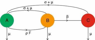
so, if , then . - Step 4.
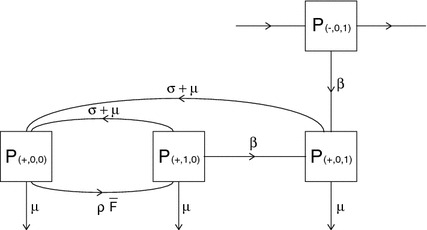
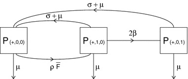
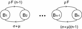
Consider . The diagram in Fig. 1 shows at once that the zero state is globally stable, i.e. if , then , . For , we have the diagram in Fig. 2, which shows that if , then , .
By continuing in this way we establish that for all with , if , then , .
Fig. 1.
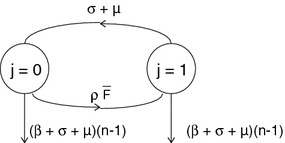
Diagram that shows that, if , then ,
Fig. 2.
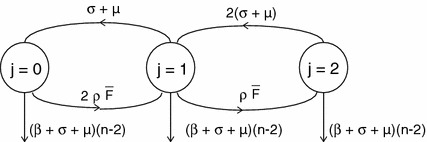
Diagram that shows that, if , then ,
It follows that we are left to deal with the stability of the following linear system:
 |
26 |
Recall definition (13) of . In the reduced linearised system (26) we are left with variables and , , . Therefore, (26) is a closed system. Furthermore, note that the dimension of the system is (where the contribution comes from the and the from the ).
The map
Order the in some appropriate way, and denote the corresponding vector by . We define a linear map from to as follows:
| 27 |
Note that maps the positive -cone to the positive cone in . In fact, if is in the interior of the positive cone, i.e. all vector elements are strictly positive, then
since for all , and for all and ,
and
since for all and we sum over . In particular it follows that if , then . We shall use this linear operator in Sect. 6.
Dynamics of the binding sites of an infectious individual: characterization of
By exploiting that an individual can be considered as a collection of binding sites that behave independently from one another as far as separation or acquiring a new partner is concerned and by using our mean field at distance one assumption, we are able to characterize in terms of binding sites. In this section we only use the interpretation of the model and we do not use the system (18) or its reduced linearisation (26). We characterize as the dominant eigenvalue of a next-generation matrix (NGM) that we construct using the interpretation of the model.
The entries in the NGM can be viewed as expected offspring values for a multi-type branching process (Jagers 1975; Haccou et al. 2005), with the two matrix-indices specifying the type at birth of, respectively, offspring and parent. Several slightly different branching processes may yield the same NGM and for the deterministic theory (which is what we deal with here) there is no need to choose one of these as ‘the’ underlying process. A branching process corresponding to the NGM is subcritical when and supercritical when . But does such a branching process indeed correspond to the linearisation of (18) in the disease free steady state? Especially for this is a nontrivial question. In Sect. 6 we will therefore prove that , as computed from the NGM, is indeed a threshold parameter with threshold value one for (18).
First, in Sect. 5.1, we consider the case . In Sect. 5.2 we generalize the transition and transmission scheme to , and in Sect. 5.3 we characterize on the level of binding sites. We conclude this section by showing in Sect. 5.4 that also has an interpretation in terms of individuals. The explicit expression for and the remainder of its derivation is left for Appendix C.
Consider the usual setting for determining , i.e. suppose that we have a population in which only a few individuals are infectious and all others are susceptible. We are interested in the expected number of secondary cases caused by one ‘typical’ infectious case.
The case
First, consider a population of individuals with partnership capacity . Then each individual has exactly one binding site. If we now consider an infectious individual, then its binding site can be in one of three states:
—free
—occupied by a susceptible partner
—occupied by an infectious partner
Please note that we recycle symbols: the here has nothing to do with the matrix of Sect. 2 and the here has nothing to do with the matrix in (10) of Sect. 3. In Fig. 3 the possible state transitions and corresponding rates for an infectious individual are given. Note that it is highly unlikely that an infectious individual acquires an infectious partner in the beginning of an epidemic, and therefore there is no transition from to .
Fig. 3.
Flow chart describing the possible transitions between states , and and their corresponding rates. Note that, in the beginning of the epidemic, only a few individuals in the population are infectious. Therefore the probability that an infectious individual acquires an infectious partner is zero. This is represented in the flowchart where there is no direct arrow from to
We can characterize by constructing an NGM that involves a transmission part and a transition part .
Recall that we use the convention that, for a transition matrix , denotes the probability per unit of time at which a transition from to i occurs (instead of the transition from i to , as it is common in the stochastic community).
The matrices and are obtained as follows. Consider an infectious individual, and order the states as , , . Then the transitions of the individual’s binding site are described by the following matrix (see Fig. 3 for its graphical representation):
| 28 |
Here is the rate at which a transition from a binding site in state to state occurs, , , and for the diagonal elements we have .
Consider an infectious individual with its binding site in state . If infects its susceptible partner , then the binding site of transits from to . This transition is represented by . In addition to this transition, an additional binding site is created. Indeed, is now also an infectious individual who has a binding site occupied by an infectious partner (namely ). This shows that one transition from to always creates one additional binding site in the population. Accordingly we define the transmission matrix :
| 29 |
Using and we can construct the NGM :
The basic reproduction number is defined as the dominant eigenvalue of (Diekmann et al. 2013, Section 7.2).
In the present case we can, quite easily, give an explicit expression for . Note that has one-dimensional range spanned by the vector . Therefore is the eigenvector corresponding to the dominant eigenvalue . We find applied to this vector by first constructing applied to this vector. This can be done by either treating it as a linear algebra problem or we can use the interpretation for it: is the mean time spent in state when starting in state , , , (in fact we only use ). We find that
and subsequently,
from which we conclude that
| 30 |
Alternatively, we can characterize by first step analysis; see Appendix A for the details or Diekmann et al. (2013, Section 7.8) or Miller et al. (2012, formula (3.1.9)) or Inaba (1997, Section 4.1). However, this does not have such a nice generalization to as the scheme does.
Generalization of the transition and transmission matrix:
Now consider the case . In this case, an individual is a collection of binding sites. These binding sites may be free, occupied by a susceptible or occupied by an infectious individual, i.e. in states , , or , respectively. An infectious individual can infect a susceptible individual in the population if it has a binding site that is occupied by a susceptible individual. In that case, that binding site becomes occupied by an infectious individual. Similar to the situation we observe that if a binding site makes a transition from ‘occupied by a susceptible individual’ to , it creates a new infectious individual in the population. However, we need to know in which states the binding sites of this new infectious individual are. Obviously, one new infectious binding site is in state , viz. the binding site still occupied by its epidemiological parent. In order to know the states of the other binding sites, we need to know the number of (susceptible) partners of this individual at epidemiological birth.
Naively, motivated by Lemma 2, one would think (as we did at first) that the number of partners of a newly infected individual is (i.e. 1 binding site in state , binding sites in state and binding sites in state ) with probability . The computation of the corresponding is rather straightforward (using the method explained in Appendix A for ). However, one can check numerically that the stability switch of the disease free steady state of (18) does not coincide with when is defined in this manner. We conclude that the premise is wrong. In retrospect this makes sense. First of all, we know that differs from , where and are defined by (7) and (8), respectively. In our model description we keep track of the number of partners of an individual. We use mean field at distance one for the partners of partners of this individual (and this shows up in the in the transmission events). So we need to do the same when characterizing and also take into account the partners of susceptible partners. Therefore, we need to extend the information that is tracked in the scheme.
We generalize the scheme of Sect. 5.1 as follows. Consider an infectious binding site. Then this binding site can be in one of states:
—free
—occupied by a susceptible partner that has partners in total,
—occupied by an infectious partner.
Let denote the collection of all states . We denote the transition matrix of the states , , , and by (see Fig. 4 for the corresponding flowchart), where
| 31 |
where denotes the dimensional zero vector, and both denote an -dimensional row vector, namely
The vector is the probability vector with elements given by (7), and is an matrix describing the transitions between the states , , and out of ; see Fig. 4 for the corresponding flowchart.
Fig. 4.
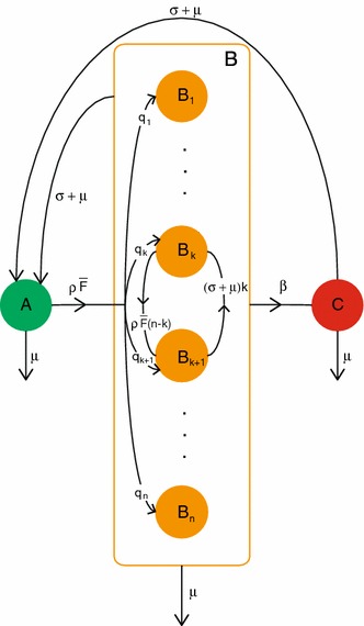
Flow chart describing the possible transitions between states , , , and and their corresponding rates
Let’s describe more carefully. The matrix describes the transitions between the and out of . Thus is an tridiagonal matrix with negative diagonal entries and positive off-diagonal entries. More specifically,
Indeed, a susceptible individual with 1 infectious and susceptible partners loses one of these susceptible partners at rate , acquires a new susceptible partner at rate , and, since it can also become infectious, lose its infectious partner, or die (these last three mark transitions out of ), the rate out of is .
The other elements of have the following interpretation. Note that, in the beginning of an epidemic, a binding site in state acquires a susceptible partner at rate . The probability that, just after the moment of acquisition, this susceptible partner has in total partners is in accordance with (7). Therefore, the rate at which a binding site in state transits to state is . In a similar way one can use the interpretation (and the flowchart in Fig. 4) to find the other entries for the matrix .
Finally, we need to construct the transmission matrix . A transmission corresponds to a transition , i.e. if an infectious individual with a binding site in infects its partner . This is included in the matrix since . The transmission matrix includes the binding sites of the newly infected partner . Concerning the binding sites of , since it is now infectious, we observe that it has one binding site in , binding sites in and binding sites will be occupied by susceptible individuals, i.e. binding sites will be in the set (see Fig. 5 for an illustration where has a binding site in that changes state to and is the newly infected individual with one binding site in , one binding site in and one binding site occupied by a susceptible individual). All that is left to specify are the states of the binding sites in , i.e. we need to know how many partners these susceptible partners of have (in Fig. 5: how many partners does have).
Fig. 5.
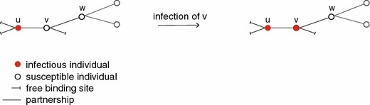
Illustration of the construction of for . Suppose we start with an individual with two binding sites in and one binding site in . Then has one susceptible partner . If infects , then will have one binding site in , one binding site in , and one binding site will be occupied by a susceptible partner . In the example, has three partners in total and therefore the binding site of would be in state . However, information about the partners of is not incorporated in our model description and therefore we assume that has three partners with probability
The probability that a partner of has partners depends on the state of , where is in state immediately after infection by . However, as another manifestation of the mean field at distance one assumption, we approximate this probability by only taking into account that the susceptible individual has at least one partner . Therefore, we assume that has partners with probability (cf. Lemma 2). In other words, we assume that a binding site of occupied by a susceptible partner, i.e. a binding site in the set , is in state with probability .
Accordingly, we define the transmission matrix as follows:
| 32 |
where is the vector
| 33 |
, where
| 34 |
and is the probability vector with components given by (8). Note that the are a linear combination of the , . We conclude that the range of is spanned by , , .
In Sect. 5.4 we shall show that we can identify the with an individual in state , which allows us to interpret in terms of individuals. But first, in Sect. 5.3, we focus on the interpretation in terms of binding sites.
in terms of binding sites
Now that we have defined the transition matrix and the transmission matrix , we are ready to define the basic reproduction ratio for as the dominant eigenvalue of the matrix
In order to underpin this, consider variables , , and , where , , and are the fractions of the total binding-site population in states , , and , respectively. Then, based on the interpretation, , , and should satisfy the following system of differential equations:
| 35 |
It follows that the zero state switches stability at . We formulate this as
Theorem 1
, defined as the dominant eigenvalue of , is a threshold parameter with threshold value one for the zero state of (35).
Note that is an matrix. Also, elements can be interpreted as the expected number of binding sites in created by one binding site in , where . This gives us an interpretation of in terms of binding sites . However, we can reduce the characterization of to a problem involving a matrix by averaging the in the right way (and this allows us to consider binding sites in , , only). We show this in the remainder of this subsection.
Consider the matrix where the , , are defined by
| 36 |
Then is also the dominant eigenvalue of . We formulate this in a theorem.
Theorem 2
, defined as the dominant eigenvalue of , where is defined by (36), is a threshold parameter with threshold value one for the zero state of (35).
Proof
We have defined as the dominant eigenvalue of and this is a threshold parameter of the linear system corresponding to the matrix according to Theorem 1. We will show that and have the same dominant eigenvalue.
The range of is spanned by three linearly independent vectors , , . If , with , , then lies in the range of , i.e. , with at least one of the . Therefore,
where the summation is over or . On the other hand, this is equal to
Since the are linearly independent, it follows that
for all . In matrix notation:
where is a three-dimensional vector, not equal to the zero vector. We conclude that if is a nonzero eigenvalue of , then is also a nonzero eigenvalue of . To find the dominant eigenvalue of , we can focus on the matrix .
Consider the definition of given by (36). This definition allows for an interpretation of the elements . Indeed, can be interpreted as the expected number of binding sites in created by one binding site in , with . Therefore, we call the NGM on the level of binding sites, and can be interpreted as the expected number of secondary cases caused by a typical newly infected binding site in the beginning of an epidemic. Note that when or equals we specify a probability distribution rather than a specific state.
The relation (36) completely characterizes the matrix . However, using the interpretation, we can give explicit expressions for the entries of ; see Appendix C. In this appendix it is also shown that, in order to find , we can reduce to a matrix and calculate the dominant eigenvalue of this smaller matrix. By combining (55)–(57), (59), and (61)–(63) we then find given as an explicit function of the model parameters.
We have characterized in terms of binding sites, both by considering all possible states and by considering . This allows for an interpretation of in terms of binding sites. As we next show, we may also interpret in terms of individuals.
in terms of individuals
The model description is on the level of individuals, so it is only sensible that, in this section, we concern ourselves with the interpretation of in terms of individuals, i.e. the interpretation of as the expected number of secondary cases caused by a typical newly infected individual (rather than binding site) in the beginning of an epidemic.
Individuals can be considered as collections of binding sites. We find the relation between the binding site level and the individual level as follows. Recall (33), where we see in the second equality that the are a linear combination of the , , and . Note that is a collection of infectious binding sites, in state , 1 in state , and in states , (and where the infectious binding site is in state with probability ). We can identify with an individual in state . Note that the are the possible states of an individual at epidemiological birth. For the case , we have only (which corresponds to the only state-at-epi-birth since an infectious individual at epi-birth is in a partnership with its epidemiological partner).
This observation allows us to also give an interpretation to for individuals. Indeed, consider , where the are characterized by
| 37 |
Element is then the expected number of secondary cases in state i caused by one infectious individual in state . Here i and are of the form , . To arrive at the interpretation of on the individual-level, we can prove that the dominant eigenvalue of (which is the NGM on individual level) equals the dominant eigenvalue of ; see Appendix E for the details.
The matrix is completely characterized by the identity (37). But, as in the case of , we can use the interpretation to give a more explicit expression for the entries of ; see Appendix F.
: equivalence of different interpretations
In Sect. 5.3 is defined as the dominant eigenvalue of . Theorem 2 states that is also the dominant eigenvalue of the -NGM , where is defined by (36), and in Appendix C we show that, in order to find the dominant eigenvalue of , we can reduce to a matrix . Finally, in Appendix E, we show that is also the dominant eigenvalue of the NGM on individual level. We summarize this in (38), where refers to ‘has the same dominant eigenvalue’.
| 38 |
In the next section we prove that defined in this way is indeed a threshold for the stability of the disease-free steady state of the nonlinear system (18), by using defined in (27) to relate the linearisation of (18) to (35).
Proof that is a threshold parameter
Recall that, using the mean field at distance one assumption, we have written down a system of differential equations to describe the transmission of the infectious disease across the dynamic network. We will refer to the system (18) of differential equations for the fractions of the population of individuals in states , as the -system. In Sect. 4 we have linearised this system around the disease-free steady state and we were able to restrict this linearised system to the fractions and . In Sect. 5 we considered binding sites of an infectious individual (in the linearisation!) and these binding sites could be in , , and . This led to the -system (35). , defined as the dominant eigenvalue of , is a threshold for the stability of the zero state of (35); this was formulated in Theorem 2. In this section we will prove that is also a threshold for the stability of the disease-free steady state of system (18). We do so by relating the reduced linearisation (26) of the -system to the -system (35).
The case
For the proof is relatively easy, since there is no distinction between ‘individual’ and ‘binding site’. As the proof provides guiding lines for the general case, we present it first.
If we write out (26) for we obtain the system of four ODE:
The consistency relation (19), which for reduces to
| 39 |
is reflected in the fact that the first and third equation of the system of ODEs are identical (recall that, for , equals and equals ). Using (39) we reduce to the three-dimensional system
To finish the proof, we only need to observe that the corresponding matrix is exactly , with defined in (28) and in (29).
Indeed, recall the three states , , and that we defined for the binding site of an infectious individual in Sect. 5.1 and the population level fractions , , in states , , and . Since individuals have exactly one binding site we identify the fractions of binding sites with fractions of individuals:
With this identification, the linearisation of the -system equals the (linear) -system. Therefore, not only is there a stability switch of the disease-free state of the -system at (see also Theorem 2), but in fact there is also a stability switch for the disease-free state of the system at .
To enhance the understanding, we present the main ingredients of the proof once more, but now by way of pictures. Figure 3 depicts the possible states and state transitions for an infectious individual. The corresponding part of the transition matrix is . The corresponding p-level variables are with indices . This part of the -vector does not form a closed system. Indeed, an individual in state has probability per unit of time to jump to , as indicated in Fig. 6.
Fig. 6.
Flow chart representing part of the linearised system of ODEs (26) for the p-level fractions
When this jump occurs, the responsible partner (the ‘epidemiological parent’) jumps from to . The interpretation underlying this last statement is mathematically reflected in the consistency relation (39). Using (39) we reduce the flow chart of Fig. 6 to the one depicted in Fig. 7. The corresponding matrix is .
Fig. 7.
Flow chart of Fig. 6 with eliminated. Note that this figure does not allow for an individual-level interpretation; the rate at which an individual in state infects its susceptible partner is (compare with Fig. 3). But the flow from population-level fraction to is with rate since it implicitly captures the inflow from
Generalization:
In general, for , we can express , , and in terms of the linearised -system by:
The explanation is as follows. An individual in state is infectious and has free binding sites and binding sites occupied by infectious partners. Summing over all possible states we obtain the number of binding sites in, respectively, states and . For the number of binding sites in state we observe that an individual in has partners in total and one infectious partner. This infectious individual therefore has a binding site occupied by a susceptible partner who has partners in total, i.e. a binding site in state . The total number of binding sites in state is therefore .
So the map defined in (27) maps the -variables to the -variables, i.e. we have the linear transformation
| 40 |
By differentiating and using (26), we obtain the linear system of differential equations (35) for , , and .
It remains to prove that the stability switch of the zero state of the -system occurs if and only if the disease-free state of the -system (18) switches stability. This will be shown in the remainder of this section.
We know that is a threshold parameter for the zero state of the -system (see Theorem 2), i.e.
| 41 |
where is the spectral bound of , i.e. , and is the spectrum of .
So in order to show that is a threshold for the disease free state of the -system, it suffices to show that
| 42 |
Here is the spectral bound of where is the matrix corresponding to the right-hand side of (26). In fact we will show that .
We will proceed as follows. First we shall prove that and are dominant eigenvalues of the matrices and , respectively, in the sense that these eigenvalues are uniquely characterized by the positivity of the eigenvector (up to a multiplicative positive constant).
We show in Lemmas 4 and 5 that and are irreducible matrices. This then allows us to conclude that the dominant eigenvalues of and are real and uniquely characterized by a positive eigenvector (see e.g. Theorem 2.5 of Seneta 1973). In other words, there exists a real eigenvalue for for which it holds that for any eigenvalue of and is uniquely defined by the positivity of the corresponding eigenvector (and similarly with replacing and replacing ).
In Lemmas 4 and 5 below we use that a matrix is irreducible if and only if variable communicates with variable () for all variables and , i.e. there is a path from to (), i.e. there are variables , , , such that , and a path from to (), i.e. there are variables , , , such that . Note that the somewhat unusual notation is due to our convention that denotes the transition from to (instead of the transition from to , as it is common in the stochastic community).
Lemma 4
is an irreducible matrix.
Proof
The flowchart describing the matrix is presented in Fig. 4. We immediately see from this figure that from any state there is a path to any other state , with . It follows that is irreducible. Since is nonnegative, also is irreducible.
Lemma 5
is an irreducible matrix.
Proof
With respect to a splitting of into components and components, is a block matrix that consists of four matrices , , , :
 |
The matrices and are non-negative matrices, not equal to the zero matrix, while and are positive off-diagonal. We show that and are irreducible, and that this implies that is irreducible.
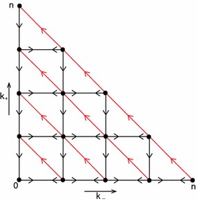
Consider . This matrix consists of the rates corresponding to the possible flows of the variables, i.e. population-level fractions of the form (and rates out of the states, that we do not need to consider here). In Fig. 8 part of the possible flows and corresponding rates are represented graphically. From Fig. 8 we immediately see that, from any variable , one can find a path to any other variable , or in other words, for all . Therefore is an irreducible matrix.
Fig. 8.
Graphical representation of part of matrix (point represents fraction ) showing that for all , i.e. is irreducible. Part of that is being ignored is e.g. the rates out of each variable leaving the system
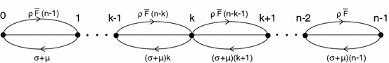
Consider the matrix . This matrix consists of the rates corresponding to the possible flows of the variables. i.e. population-level fractions of the form . In Fig. 9 a graphical representation of part of the possible flows are given and in Fig. 10 the rates corresponding to these flows are given. These figures show (literally) that is irreducible.
Fig. 9.
Graphical representation of the possible flows incorporated in the matrix (coordinate represents fraction ), ignoring the death rate out of each fraction
Fig. 10.
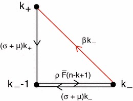
Rates corresponding to the flows of Fig. 9, ignoring the death rate out of each variable
Finally, consider two variables , of the matrix . We show that .
Since and are non-negative and non-zero, there are variables , , , such that and . Note that, in terms of interpretation, the nonzero elements of correspond to infection of individuals by one of their partner, i.e. transitions with rate from fractions to . The nonzero elements of correspond to the feed into the category via the terms from fractions .
We find a path from through and , i.e.
and a path from through and , i.e.
Note that the paths , , , and exist since and are irreducible.
Since any two variables and of communicate, i.e. , is irreducible.
We now have all the ingredients to prove that is a threshold parameter for the disease free state of (18).
Since is an irreducible positive off-diagonal matrix, we know that has a real dominant eigenvalue with corresponding positive eigenvector , i.e.
Then how does this relate to ? On the one hand we find that
on the other hand and (35) holds. Therefore
| 43 |
and it follows that
We have seen in Sect. 4 that if is strictly positive then so is . Furthermore, since is an irreducible positive off-diagonal matrix (see Lemma 4), the Malthusian parameter of is uniquely characterized by a positive eigenvector. Therefore is also the Malthusian parameter of with corresponding eigenvector , i.e.
| 44 |
Finally, (42) together with Theorem 2 shows that is a threshold parameter of the -system.
Characterization of the Malthusian parameter ()
In this section we characterize the initial exponential growth rate (recall (44)). The Malthusian parameter satisfies
So lies in the range of , i.e.
with
| 45 |
where the are some constants, not all equal to zero, and the are defined in (34), . This is equivalent to
Therefore
where is defined by (45), so
| 46 |
Since the range of is spanned by , we also have that, for certain constants ,
| 47 |
The Malthusian parameter then needs to satisfy
where is a matrix characterized by (47), with matrix elements depending on the unknown . Identity (47) fully characterizes elements , but, as in the case of and , we can use the interpretation to give explicit expressions for the entries of , in the last paragraph of Appendix C we outline how this can be done.
Finally, consider the case , then satisfies
| 48 |
where and are defined in (28) and (29), respectively. Since the range of is spanned by , we see that . We find that
It then follows from (48) that we find by solving the following third-order polynomial in :
Looking back and ahead
The overall aim of our research is to formulate and analyse models for the spread of an infectious disease across a network that is dynamic in the double sense that individuals come (by birth) and go (by death) and that links/partnerships are formed and broken. In particular our aim is to investigate the role of concurrency in the spread of sexually transmitted infections.
In Leung et al. (2012) we introduced a class of doubly dynamic network models that are relatively simple to describe, that involve just a few parameters, and for which one can calculate many statistics exactly in explicit detail. The next step, taken here, is superimposing the spread of an infection. In order to retain the simplicity, we again characterize individuals by their dynamic degree (i.e. the current number of their partners), but now include the disease status ( versus ) of the individual itself and of its partners. In this bookkeeping scheme we need to account for the infection of a partner by one of its other partners, but the scheme itself does not provide information about partners of partners. Thus we faced a closing problem. The mean field at distance one assumption provided a natural solution.
Originally we thought that this was an assumption because we had not yet found a way to prove it. In a late stage Pieter Trapman pointed the way to the current Appendix B, showing that the assumption is inconsistent with the model itself. We then realised that, in essence, our bookkeeping scheme constitutes a first order description that we close by making the (inconsistent) mean field at distance one assumption. So the deterministic system studied here provides at best an approximation to the large system size limit of a stochastic model.
The great advantage of the deterministic system of dimension is that it is amenable to analysis. The fact that binding sites operate to some extent independently from each other enables a reduction of the dimension from to in the characterization of . Indeed, we characterized the basic reproduction number as the dominant eigenvalue of a matrix with elements describing the expected numbers of newly infected binding sites of three different types generated by one infected binding site of either type during its life time. We could then further reduce the matrix to a matrix which lead to an explicit expression for the dominant eigenvalue . We also verified that the basic reproduction number defined in this way is indeed a threshold parameter for the stability of the disease free steady state of the nonlinear system of model equations. This is done by establishing a relationship between the exponential growth rate of the epidemic in the linearised system and the quantity on the level of binding sites.
The characterization of and opens up the route for investigating the impact of concurrency on the transmission of the infection in the dynamic network. We can now study how and depend on the capacity when fixing all other parameters at constant values. Furthermore, the relationship between concurrency measures on the one hand and , , and the endemic steady state on the other, can be analysed. This will be explored in a follow-up paper. (Concerning the endemic steady state, we will need to derive the equations that characterize it, to investigate the uniqueness and to prove that existence requires .)
There are a number of generalisations of the network model that are both useful and feasible. The extension to a heterosexual population requires only the distinction between males and females and some assumptions on the symmetry or asymmetry in rates and partnership capacity between the two sexes. We expect that all results presented here carry, mutatis mutandis, over to that situation. No doubt the model can also be extended to the situation that is a random variable with a prescribed distribution.
Other generalisations pertain to the description of infectiousness. An obvious example is a model with two consecutive stages and , where infectiousness is characterised by in stage . Other compartmental epidemic models could be considered as well, such as and . Inclusion of the impact of the disease on mortality is very relevant in the context of HIV. Unfortunately it might turn out to be very hard.
The most stringent limitation of our framework is the assumption that having a partner does not influence an individual’s propensity to enter into a new partnership or its contact rate in other ongoing partnerships. This is clearly at odds with reality (although equally clearly it is an impossible task to disentangle the manifold ways in which dependence ‘works’ in reality). Dependence destroys the basis on which our analytic approach rests.
Be that as it may, we view the work presented here as a first step towards a framework for studying the impact of dynamic network structure on the transmission of an infectious disease.
Acknowledgments
We thank Pieter Trapman, Martin Bootsma, and Hans Metz for useful ideas and discussions. We thank two anonymous referees for helpful suggestions. KYL is supported by the Netherlands Organisation for Scientific Research (NWO) through research programma Mozaïek, 017.009.082.
Appendix A: for : alternative method
We can also characterize for the case in the following way. An individual at epidemiological birth is in state with probability one (since it has its epidemiological parent as partner) and each time it visits (which is only possible by jumping from to since the probability to encounter an infectious individual is zero at the beginning of an epidemic) a new infectious individual is created; recall Fig. 3. So, for , we simply need to count the expected number of times to visit when starting in . This can be done by exploiting the Markov property:
| 49 |
where is the probability to ever enter state when starting in state . Let denote the probability to ever enter state when starting in , . We find by first-step analysis:
Solving for we find
This yields the same expression (30) as the scheme does.
Appendix B: Correlation between the states of two partners
Consider a randomly chosen partnership. For convenience we call the individuals in the partnership and . Then, without knowing anything about , the probability that is in state , , is given by (Lemma 2), i.e.
In other words, is the probability that an individual is in state given that it has at least one partner.
Let’s study this partnership in more detail. The states of and are independent of each other at the moment when the partnership is formed, i.e.
cf. assumption (7).
As long as we condition on the existence of the partnership the remaining binding sites of behave independently of the remaining binding sites of and consequently there is independence of the states of and at any time in the partnership, i.e.
However, if we do not specify the duration so far of the partnership, then we find dependence between the states of and :
Here the density accounts for the conditioning on the partnership remaining in existence. We show the inequality with explicit calculations for . In this case, individuals can have 0, 1, or 2 partners. Choose a partnership at random from the population and label the partners and . Since , and both have one additional binding site that can be either free or occupied. This gives us three possible states for the partnership , we denote these states by , , and ; see Fig. 11.
Fig. 11.
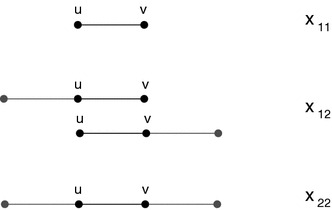
The three possible configurations for the partnership concerning additional partners when
Let denote the probability distribution for the configuration of the partnership at time given that exists for the period under consideration.
At the probability distribution of the different configurations is given by
Given that the partnership exists for the time interval under consideration, the transitions and the corresponding rates are represented by the flowchart in Fig. 12. We denote the corresponding transition matrix by .
Fig. 12.
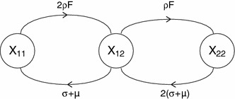
The flowchart for the three possible configurations for the partnership concerning additional partners given that exists for the period under consideration
Note that the ‘age’ of the partnership is exponentially distributed with parameter . Therefore the probability distribution for the configuration of partnership at the moment we pick the partnership from the pool of partnerships is
| 50 |
| 51 |
where
The states of and are independent of one another iff
Note that if and corresponds to a dynamic network without demography. One should, however, not conclude that demography necessarily leads to correlation. We assumed that individuals are born single. One can think of other ways of incorporating demography, e.g. individuals having partners at birth with probability equal to the degree distribution (Kamp 2010). Adopting this rule creates a partnership network where, when disease is not considered, the correlation is zero between the degrees of two partners [in essence this rule makes ‘death’ the same as rewiring of partnerships after an exponentially distributed amount of time and then basically a dynamic network in a closed population is considered (Miller et al. 2012)].
Appendix C: The matrix elements of and a characterization of by a matrix
In this appendix we use the interpretation to guide us in deriving explicit expressions for the and in that way we derive an explicit expression for .
First of all, as explained below, the following equalities hold:
| 52 |
| 53 |
| 54 |
Indeed, if we multiply the right-hand side of each of these equalities with the matrix , where is defined in (31), we obtain , .
The elements , , also have an interpretation. The interpretation of is as follows. Consider a binding site in state . The probability for the binding site to be in state in the time interval is
where is defined in (28). It enters the set at rate . The probability that the binding site is in state upon entering is . The probability to remain in in the time interval is the th component of
By integrating over all possible we find the expectation:
The th component is then the mean time a binding site that starts in state will spend in state . Similarly, one can interpret .
Finally, we show how to derive (53) by exploiting the interpretation of (this is the most complicated case and it involves all building blocks for the other cases).
First note that is the probability to be in state at time when one starts life in state , so , is the mean time spent in state when the binding site starts its life in state . Therefore
There are flows out of to and with rates and , respectively. There is also a flow in to from with rate . Note that the transition matrix between state , set , and state is exactly , where is defined in (28).
We shall use the inverse in the following calculations. Using linear algebra or interpretation, we obtain
The mean time a binding site born in one of the states in the set , spends in state is given by
while the mean future time a binding site presently in spends in state is
To determine the mean time spent in the set , when starting life in , is a bit more complicated. First of all, a binding site that starts life in starts life in state with probability , . The mean time it then spends in state without leaving the set is given by
Next, the binding site in leaves and enters with probability
If that is the case, then the mean future time it spends in is, by first step analysis,
Similarly, the probability to enter state from is
and the mean time it will spend in is
Therefore, the mean time spent in state after leaving is
This explains (53).
The matrix is given by (32). By multiplying with (52), (53), and (54), we obtain the first column of
| 55 |
the second column of is given by
| 56 |
and the third column is
| 57 |
Note that the elements , involve the vectors and .
We can simplify the sums and . Note that
since is the mean time to spent in state when starting life in state , by summing over all possible states , we obtain the mean time to spent in when starting in some state (this is of course equal to 1 over the rate of leaving ). Therefore, for any probability distribution ,
where the last equality holds since is a probability distribution. So
| 58 |
which we can use to simplify .
Observe that the sum of the first and second row of is times the third row of , i.e.
and the third column is a multiple of the first column, i.e.
So we find that, of the three eigenvalues that has, at least one equals zero. Moreover, using (58),
and
To find the dominant eigenvalue of we can therefore reduce to the matrix :
| 59 |
Note that
| 60 |
where is the probability distribution or , and we have used (58) in the second equality. Therefore, the only ingredients left in order to arrive at a completely explicit expression for the dominant eigenvalue of the matrix are explicit expressions for the sums and .
In the remainder of this appendix we show that
| 61 |
and
| 62 |
where
| 63 |
We obtain an explicit expression for by using (60) and plugging (61) and (62) (together with (63)) into (55) and (56). Next, plug these into (59) and use that the dominant eigenvalue of a matrix is
(where tr and det denote the trace and determinant of , respectively).
Finally, in the remainder of this appendix we will show (61) and (62) by straightforward computations that we divide up in four lemma’s (for the first of these we only sketch the proof).
We need the following ingredients. Let be the matrix corresponding to the state transitions between the states , ; see Fig. 13. Then
Furthermore, denotes the fundamental solution of
| 64 |
We also use the relationship between and :
| 65 |
(see proof Leung et al. 2012, Lemma 2).
Fig. 13.
State transitions and corresponding rates between states ; the corresponding transition matrix is denoted
We need the probability distribution for : where the superscript is to distinguish the probabilities from general .
| 66 |
Finally, we use two probabilities for binding sites. Consider one binding site. Conditioning on the individual staying alive till at least time , and denote the probabilities that the binding site is occupied at time , given that, respectively, it was free or occupied at time . So , , satisfies
with initial conditions and . Solving these, we find
| 67 |
Lemma 6
| 68 |
Sketch of proof
Consider a randomly chosen partnership between two individuals and . Then is the probability for to be in state given that it starts life in (here: ‘life starts’ at the moment is formed). Then is the expected number of partners of , minus partner , at time given that started life in . Conditioning on the existence of , the other binding sites of behave independently of one another.
Since starts life in state , there are binding sites that have probability to be occupied at time and binding sites that have probability to be occupied at time . Therefore, the expected number of occupied binding sites of minus the binding site occupied by at time is exactly the right hand side of (68).
We now consider the expected number of ‘other’ partners of an individual that just acquired a new partner in the following lemma.
Lemma 7
with given by (66).
Proof
The probability is given by (7) with
Then
If we now take the sum , then we obtain
which we wanted to show.
Lemma 8
where is the positive constant (63).
Proof
We combine Lemmas 6 and 7.
Finally, one can use (66) and (67) in the last step to arrive at the explicit expression.
Lemma 9
Proof
Putting all the pieces together, we obtain
and for the sum involving , we use (65), and then find
Finally, we note that we can use the method described in this appendix to find explicit expressions for the matrix entries of the matrix , that are characterized by identity (47). Note that we can find expressions for the , by simply replacing by in the calculations in this appendix. This allows us to characterize . We refrain from elaborating the details.
Appendix D: Mean field at distance one—bounds for
As explained in the main text, the mean field at distance one assumption is a moment closure approximation as we ignore certain correlations between the states of two individuals in a partnership. One may wonder how well ‘the real ’ (presuming it can be defined, when no assumption is made about the degree distribution of the partners of an individual at epi-birth) is approximated by as derived under the mean field at distance one assumption. Note that here we focus on the mean field at distance one assumption in the linearised system only.
In this appendix we provide lower- and upper bounds for ‘the real ’ for the case with numerical values presented in Fig. 14.
Fig. 14.
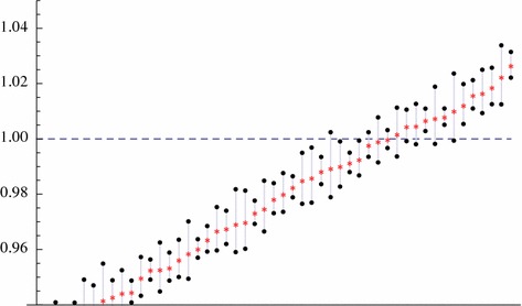
For different values of parameters , , , , the basic reproduction number is determined together with a lower and an upper bound for ‘the real ’. We focus here on parameter values for which lies around threshold value 1
Consider a randomly chosen partnership with partners and . Assume that the partnership is formed at time . Then, as long as we condition on the existence of partnership , the states of and are independent from one another at time (as also explained in Appendix B). The probability that is in state 1 or 2 at time is given by the probability distribution
, where
For , this yields initial condition , for we obtain probability distribution
Then
(note that the equality holds since the degrees of and are independent of one another as long as we specify the duration of the partnership ). Therefore
| 69 |
(recall that we condition on the existence of partnership ). Under the mean field at distance one assumption, we say that
As we will explain now, (69) provides us with a bandwidth for ‘the real ’ (in which the mean field at distance one also falls).
The mean field at distance one assumption manifests itself in the distribution , which plays a role in elements and . For , we find and .
If we replace by a probability distribution in (59) (and keep all other elements equal) then we deal with , . Using (58) we find that holds so we can eliminate . (All other elements in (59) do not concern the mean field at distance one assumption, so for any assumption on the degree distribution of the partners of an individual at epi-birth, these will be the same.) We can then express the dominant eigenvalue of as a function of using the explicit formula for the dominant eigenvalue of a matrix. This is then a monotonically increasing function of .
Furthermore, one can check that
where (note that ), so is a monotonically increasing function of . Using (69) we then find
and we find a lower (upper) bound by replacing by () for ‘the real ’ which we can compare with the dominant eigenvalue of (59). We evaluate this numerically in Fig. 14 to get some indication of how well the mean field at distance assumption performs.
We believe that this can be generalized to obtain a bandwidth for for by considering expected values but we have not elaborated the details.
Appendix E: The dominant eigenvalue of equals the dominant eigenvalue of
We have defined on the binding-site level as the dominant eigenvalue of a NGM . In this section we prove that and , the NGM on the individual level, have the same dominant eigenvalue . Therefore, has an interpretation on both the binding site and the individual level.
Lemma 10
and have the same dominant eigenvalue .
Proof
With the matrix given by
| 70 |
the identity
| 71 |
holds. Since , , , , , we know that and for all . Therefore and are primitive matrices.
Now suppose that is the eigenvector corresponding to eigenvalue , then implies that
Since can be chosen as a strictly positive vector (as it belongs to the dominant eigenvalue of a primitive matrix) and is non-negative and non-zero, is also strictly positive. Therefore, is the (strictly positive) eigenvector corresponding to the eigenvalue of . Since is primitive, it must also be the dominant eigenvalue of .
On the other hand, suppose is the eigenvector corresponding to the dominant eigenvalue of (where denotes the transpose of ), so . Then we can choose strictly positive, as is primitive. Then
So we see that is an eigenvalue of (and therefore also of ) with strictly positive eigenvector . Therefore, is the dominant eigenvalue of , i.e. .
Appendix F: Characterizing the matrix elements
The matrix elements of the matrix are uniquely characterized in (37). However, as in the case with , we can give more explicit expressions for using the interpretation.
Indeed, can be interpreted as the expected number of secondary cases in state i caused by one individual in state , where i and are of the form , . A newly infected individual in state has susceptible partners, where each of these partners is in state with probability (as a consequence of the mean field at distance one assumption). The probability that an individual in state gets infected and has state-at-epi-birth is . On top of the secondary cases caused by infecting existing partners, the newly infected individual can also cause secondary cases among the partners that it acquires after epi-birth. A newly acquired partner is in state with probability , and the probability that this individual gets infected and has state-at-epi-birth i is again . The expected additional lifetime number of partners of an individual in state is times the expected lifetime number of partners of a free binding site plus times the expected additional lifetime number of partners of an occupied binding site, where the expected lifetime number of partners of a free binding site is
while the expected additional lifetime number of partners of an occupied binding site is
Using this interpretation of the matrix elements we find
| 72 |
with and are -dimensional vectors, where is the second row of the matrix defined in (70), i.e.
, and
In order to prove that , defined by (37), satisfies (72), we use results from Appendix C. First of all, can be written as
Therefore,
Now, we can expand this using the characterization of the of Appendix C. The coefficient of is
On the other hand,
Therefore
Contributor Information
Ka Yin Leung, Email: k.y.leung@uu.nl.
Mirjam Kretzschmar, Email: m.e.e.kretzschmar@umcutrecht.nl.
Odo Diekmann, Email: o.diekmann@uu.nl.
References
- Altmann M. Susceptible-infected-removed epidemic models with dynamic partnerships. J Math Biol. 1995;33:661–675. doi: 10.1007/BF00298647. [DOI] [PubMed] [Google Scholar]
- Altmann M. The deterministic limit of infectious disease models with dynamic partners. Math Biosci. 1998;150:153–175. doi: 10.1016/S0025-5564(98)00012-1. [DOI] [PubMed] [Google Scholar]
- Ball F, Neal P. Network epidemic models with two levels of mixing. Math Biosci. 2008;212:69–87. doi: 10.1016/j.mbs.2008.01.001. [DOI] [PubMed] [Google Scholar]
- Bansal S, Read J, Pourbohloul B, Meyers LA. The dynamic nature of contact networks in infectious disease epidemiology. J Biol Dyn. 2010;4:478–489. doi: 10.1080/17513758.2010.503376. [DOI] [PubMed] [Google Scholar]
- Barbour AD, Reinert G. Approximating the epidemic curve. Electron J Probab. 2013;18:1–30. doi: 10.1214/EJP.v18-2557. [DOI] [Google Scholar]
- Britton T, Lindholm M. Dynamic random networks in dynamic populations. J Stat Phys. 2010;139:518–535. doi: 10.1007/s10955-010-9952-5. [DOI] [Google Scholar]
- Britton T, Lindholm M, Turova T. A dynamic network in a dynamic population: asymptotic properties. J Appl Probab. 2011;48:1163–1178. doi: 10.1239/jap/1324046025. [DOI] [Google Scholar]
- Decreusefond L, Dhersin J-S, Moyal P, Tran VC. Large graph limit for an SIR process in random network with heterogeneous connectivity. Ann Appl Probab. 2012;22:541–575. doi: 10.1214/11-AAP773. [DOI] [Google Scholar]
- Diekmann O, de Jong MCM, Metz JAJ. A deterministic epidemic model taking account of repeated contacts between the same individuals. J Appl Probab. 1998;35:448–462. doi: 10.1239/jap/1032192860. [DOI] [Google Scholar]
- Diekmann O, Heesterbeek JAP, Britton T. Mathematical tools for understanding infectious disease dynamics. Princeton: Princeton University Press; 2013. [Google Scholar]
- Dietz K, Hadeler KP. Epidemiological models for sexually transmitted diseases. J Math Biol. 1988;26:1–25. doi: 10.1007/BF00280169. [DOI] [PubMed] [Google Scholar]
- Eaton JW, Hallett TB, Garnett GP. Concurrent sexual partnerships and primary HIV infection: a critical interaction. AIDS Behav. 2011;15:687–692. doi: 10.1007/s10461-010-9787-8. [DOI] [PMC free article] [PubMed] [Google Scholar]
- Ferguson NM, Garnett GP. More realistic models of sexually transmitted disease transmission dynamics. Sex Transm Dis. 2000;27:600–609. doi: 10.1097/00007435-200011000-00008. [DOI] [PubMed] [Google Scholar]
- Goodreau SM. A decade of modelling research yields considerable evidence for the importance of concurrency: a response to Sawers and Stillwaggon. J Int AIDS Soc. 2011;14:12. doi: 10.1186/1758-2652-14-12. [DOI] [PMC free article] [PubMed] [Google Scholar]
- Haccou P, Jagers P, Vatutin VA. Branching processes. Variation, growth, and extinction of populations. Cambridge: Cambridge University Press; 2005. [Google Scholar]
- Heijne JC, Althaus CL, Herzog SA, Kretzschmar M, Low N. The role of reinfection and partner notification in the efficacy of Chlamydia screening programs. J Infect Dis. 2011;203:372–377. doi: 10.1093/infdis/jiq050. [DOI] [PMC free article] [PubMed] [Google Scholar]
- House T, Keeling MJ. Insights from unifying modern approximations to infections on networks. J R Soc Interface. 2011;8:67–73. doi: 10.1098/rsif.2010.0179. [DOI] [PMC free article] [PubMed] [Google Scholar]
- Inaba H (1997) Advances in mathematical population dynamics: molecules, cells and man. Calculating for HIV infection via pair formation. World Scientific, pp 355–382
- Jagers P. Branching processes with biological applications. New York: Wiley; 1975. [Google Scholar]
- Kamp C. Untangling the interplay between epidemic spread and transmission network dynamics. PLoS Comput Biol. 2010;6:e1000984. doi: 10.1371/journal.pcbi.1000984. [DOI] [PMC free article] [PubMed] [Google Scholar]
- Kenyon C, Colebunders R. Strong association between point-concurrency and peak HIV prevalence. J Infect Dis. 2012;16:e826–e827. doi: 10.1016/j.ijid.2012.05.008. [DOI] [PubMed] [Google Scholar]
- Kiss IZ, Berthouze L, Taylor TJ, Simon PL (2012) Modelling approaches for simple dynamic networks and applications to disease transmission models. Proc R Soc A 468:1332–1355
- Kretzschmar M, Dietz K. The effect of pair formation and variable infectivity on the spread of an infection without recovery. Math Biosci. 1998;148:83–113. doi: 10.1016/S0025-5564(97)10008-6. [DOI] [PubMed] [Google Scholar]
- Kretzschmar M, Morris M. Measures of concurrency in networks and the spread of infectious disease. Math Biosci. 1996;133:165–195. doi: 10.1016/0025-5564(95)00093-3. [DOI] [PubMed] [Google Scholar]
- Kretzschmar M, Jager JC, Reinking DP, Van Zessen G, Brouwers H. The basic reproduction ratio R0 for a sexually transmitted disease in a pair formation model with two types of pairs. Math Biosci. 1994;124:181–205. doi: 10.1016/0025-5564(94)90042-6. [DOI] [PubMed] [Google Scholar]
- Leung KY, Kretzschmar MEE, Diekmann O. Dynamic concurrent partnership networks incorporating demography. Theor Popul Biol. 2012;82:229–239. doi: 10.1016/j.tpb.2012.07.001. [DOI] [PubMed] [Google Scholar]
- Lindquist J, Ma J, van den Driessche P, Willeboordse FH. Effective degree network disease models. J Math Biol. 2011;62:143–164. doi: 10.1007/s00285-010-0331-2. [DOI] [PubMed] [Google Scholar]
- Lurie MN, Rosenthal S. Concurrent partnerships as a driver of the HIV epidemic in sub-Saharan Africa? The evidence is limited. AIDS Behav. 2010;14:17–24. doi: 10.1007/s10461-009-9583-5. [DOI] [PMC free article] [PubMed] [Google Scholar]
- Miller JC, Volz EM. Incorporating disease and population structure into models of SIR disease in contact networks. PLoS ONE. 2013;8:e69162–e69162. doi: 10.1371/journal.pone.0069162. [DOI] [PMC free article] [PubMed] [Google Scholar]
- Miller JC, Slim AC, Volz EM. Edge-based compartmental modelling for infectious disease spread. J R Soc Interface. 2012;9:890–906. doi: 10.1098/rsif.2011.0403. [DOI] [PMC free article] [PubMed] [Google Scholar]
- Morris M, Kretzschmar M. Concurrent partnerships and the spread of HIV. AIDS. 1997;11:641–648. doi: 10.1097/00002030-199705000-00012. [DOI] [PubMed] [Google Scholar]
- Morris M, Kretzschmar M. A microsimulation study of the effects of concurrent partnerships on the spread of HIV in Uganda. Math Popul Studies. 2000;8:109–133. doi: 10.1080/08898480009525478. [DOI] [Google Scholar]
- Powers KA, Ghani AC, Miller WC, et al. The role of acute and early HIV infection in the spread of HIV and implications for transmission prevention strategies in Lilongwe, Malawi: a modelling study. Lancet. 2011;378:256–268. doi: 10.1016/S0140-6736(11)60842-8. [DOI] [PMC free article] [PubMed] [Google Scholar]
- Reniers G, Watkins S. Polygyny and the spread of HIV in sub-Saharan Africa: a case of benign concurrency. AIDS. 2010;24:299–307. doi: 10.1097/QAD.0b013e328333af03. [DOI] [PMC free article] [PubMed] [Google Scholar]
- Seneta E. Non-negative matrices. An introduction to theory and applications. London: George Allen & Unwin Ltd; 1973. [Google Scholar]
- Tanser F, Barnighausen T, Hund L, Garnett GP, McGrath N, Newell ML. Effect of concurrent sexual partnerships on rate of new HIV infections in a high-prevalence, rural South African population: a cohort study. Lancet. 2011;378:247–255. doi: 10.1016/S0140-6736(11)60779-4. [DOI] [PMC free article] [PubMed] [Google Scholar]
- Taylor M, Simon PL, Green DM, House T, Kiss IZ. From Markovian to pairwise epidemic models and the performance of moment closure approximations. J Math Biol. 2012;64:1021–1042. doi: 10.1007/s00285-011-0443-3. [DOI] [PubMed] [Google Scholar]
- Watts CH, May RM. The influence of concurrent partnerships on the dynamics of HIV/AIDS. Math Biosci. 1992;108:89–104. doi: 10.1016/0025-5564(92)90006-I. [DOI] [PubMed] [Google Scholar]
- Xiridou M, Geskus R, De Wit J, Coutinho R, Kretzschmar M. The contribution of steady and casual partnerships to the incidence of HIV infection among homosexual men in Amsterdam. AIDS. 2003;17:1029–1038. doi: 10.1097/00002030-200305020-00012. [DOI] [PubMed] [Google Scholar]