

Abstract
Behavioral scientists have historically relied on static modeling methodologies. The rise in mobile and wearable sensors has made intensive longitudinal data (ILD)—behavioral data measured frequently over time—increasingly available. Consequently, analytical frameworks are emerging that seek to reliably quantify dynamics reflected in these data. Employing an input-output perspective, dynamical systems models from engineering can characterize time-varying behaviors as processes of change. Specifically, ILD and parameter estimation routines from system identification can be leveraged together to offer parsimonious and quantitative descriptions of dynamic behavioral constructs. The utility of this approach for facilitating a better understanding of health behaviors is illustrated with two examples. In the first example, dynamical systems models are developed for Social Cognitive Theory (SCT), a prominent concept in behavioral science that considers interrelationships between personal factors, the environment, and behaviors. Estimated models are then obtained that explore the role of SCT in a physical activity intervention. The second example uses ILD to model day-to-day changes in smoking levels as a craving-mediated process of behavior change.
I. Introduction
Historically, accurately quantifying human behavior with respect to time had met with limited success. This is largely due to methodological challenges associated with frequent measurement of behavioral constructs, which helped lead to behavioral science research's reliance on tightly controlled laboratory or clinical settings and correlational epidemiological studies for studying behavior change. As a result, hypothesized mechanisms of behavior change have largely emerged from static analyses of cross-sectional data [1].
Recent advances in mobile technologies (e.g., smart phones) and wearable sensors (e.g., wearable accelerometers) have facilitated cost-effective collection of what behavioral scientists call “intensive longitudinal data” (ILD)—frequent measurements of behavioral constructs (e.g., how long an individual engages in physical activity, levels of motivation to engage in physical activity), including continuous-time and real-time measurement of behaviors [2], [3]. With the rise in the availability of ILD, behavioral scientists have been increasingly pursuing opportunities to better understand how behaviors and related constructs change over time and how exogenous variables such as environmental factors and therapeutic interventions affect these dynamics. Furthermore, ILD offers a means to develop richer descriptions of theorized behavior change mechanisms, which could help validate and guide revisions to such hypothesized mechanisms.
Contrasting traditional statistical behavioral science methods, analytical frameworks have recently emerged that are better suited to model dynamic phenomena captured in ILD. Methods from engineering offer one such approach for characterizing dynamic behaviors as processes of change [1], [4], [5]. Specifically, continuous-time differential equation models that employ an input-output perspective—i.e., dynamical systems models—are well suited for such analyses. For example, recent work estimated low order differential equations to describe dynamics observed in pain management [4], smoking cessation [5], and physical activity intervention [1] studies. The dynamic models developed in these efforts draw from ILD and parameter estimation routines from system identification to estimate gains, which quantify the net response of a behavioral outcome variable (e.g., duration of daily physical activity, self-reported urge to smoke cigarettes) to unit changes in input variables (e.g., unit doses of behavioral counseling intended to promote healthy behaviors), time constants, which quantify the speed of the outcome variable's response, system zeros, which indicate shape of response, and more [6], [7]. Employing this approach to characterize time-varying behaviors benefits from the fact that system identification routines are reliable and mature, having been applied within engineering settings for decades [6], [7], and have been precoded in commercially-available products such as MATLAB [7], [8]. Furthermore, dynamical systems models often act as the basis for the design of control algorithms that seek to automate optimal operation of industrial systems; the connection to control theory suggests that incorporating this engineering modeling approach into behavioral science settings offers the opportunity to develop novel closed-loop behavioral interventions (see [1], [5] and articles referencing [4], [9]).
Through two case studies, this article summarizes the usefulness of dynamical systems modeling and system identification for leveraging ILD in order to better understand human behavior change: Section II outlines a dynamical systems approach for characterizing Social Cognitive Theory—an influential concept in behavioral science that is based in learning theory [10]—in the context of a physical activity intervention (described in detail in [1]); Section III describes use of an engineering approach for examining smoking behavior change and the role of statistical mediation—a hypothesized mechanism of change commonly studied in the social and behavioral sciences [11] (described in detail in [5]); finally, Section IV comments on future research.
II. Case Study I: Social Cognitive Theory & Physical Activity Behaviors
Growing out of learning theory, Social Cognitive Theory (SCT) revolves around the idea of triadic reciprocity, which considers inter-relationships between personal factors (e.g., cognition, biology), the environment, and behaviors, seeking to explain how internal and external factors lead an individual to engage in target behaviors [1], [10]. Specifically, there are five fundamental components of SCT, which are seen as outputs in a dynamical systems sense (referred to as η1…6); SCT attributes changes in these components to eight external and internal factors, which are treated as exogenous inputs in dynamical systems models (represented as ξ1…8):
Self-management skills (η1) - complex set of behaviors that increases an individual's potential for engaging in a target behavior, e.g., self-monitoring, goal setting.
Outcome expectancy (η2) - perceived likelihood that performing a target behavior will result in specific outcomes.
Self-efficacy (η3) - perceived ability to engage in a target behavior.
Behavior (η4) - target action of interest.
Behavioral outcomes (η5) - results of target behavior, e.g., weight loss due to increased physical activity.
Cue to action (η6) - trigger to engage in a behavior.
Skills training (ξ1) - activities that alter an individual's self-management abilities.
Observed behavior (ξ2) - learning resulting from observing the results of others' behaviors.
Perceived social support (ξ3).
Cues to action (ξ4, ξ8) - internal and external triggers, respectively, that influence engagement in a behavior.
Perceived obstacles (ξ5).
Intrapersonal states (ξ6) - physical, mental, and emotional states that influence self-efficacy.
Environmental context (ξ7).
Dynamical systems models describing behavior change via an SCT-based mechanism stem from a connection to production-inventory systems [1], [4], [9]: Fig. 1 depicts SCT in terms of a fluid analogy [1]. Here, the five outputs, η1…6, are represented as fluid inventories (tanks), which accept inflow streams of fluid. The manner in which the level of fluid in an inventory changes in response to changes in inflows represents the way in which Self-efficacy, Behavior, etc., respond to changes in the respective factors that influence them. The specific inflows to each individual inventory depicted in Fig. 1 reflect the relationships that formally define SCT (see [10]). For example, the Self-management skills inventory (η1) accepts three inflow streams: Skills training (ξ1), which is an external input to the overall system and is represented as an exogenous input stream flowing at a known and controlled rate; a portion of the outflow stream from the Behavior inventory, which reflects the inter-relationship between the Self-management skills and Behavior constructs; and the disturbance input ζ1, which represents the unmodeled factors that influence Self-management skills. Altogether, the six inventories in Fig. 1 are inter-connected to reflect the triadic reciprocity proposed in [10].
Fig. 1.

Fluid analogy describing behavior change according to the mechanism constituting SCT.
An engineering model of SCT is developed by applying the conservation of mass principle (which is used as a general accounting principle here) to the inventories and assuming the dynamic response of each output to changes in inputs are adequately represented by first order differential equations. The result is a system of differential equations:
| (1) |
| (2) |
| (3) |
| (4) |
| (5) |
| (6) |
where the left hand side of the equations are transition terms (units of η), i.e., the change in the level of an inventory (dη [units of η]) over some time (dt [units of time]), is related to the speed at which the inventory level responds to a unit change in the tank's inflows and outflows (time constant, τ); ηi and ξi are the output and input variables, respectively, that are fundamental to SCT; γij is the gain between input variable ξi and output variable ηj; βmn is the gain for the interrelationship between variable ξm and ξn; and ζi is an unmodeled disturbance that affects output ηi [1].
SCT is among the most influential theories in behavioral science, and has been recently examined in the context of a physical activity intervention [1]. Specifically, estimated dynamic models were obtained using averaged ILD from six participants in the Mobile Interventions for Lifestyle Exercise and Eating at Stanford (MILES) study [12]. These models focused on a two-input, two-output problem: Self-efficacy, as recorded on a 1-11 point scale by participants via smart phone, and Behavior, the total number of steps taken per day as measured by an accelerometer, were the outputs of interest. The two inputs were intervention components: Skills training, consisting of tips for engaging in a target behavior delivered as reading material via the ‘mtrack’ smart phone application (recorded as seconds spent reading the tips), and external cues, consisting of smart phone reminders to set new physical activity goals (recorded as the number of reminders sent to a participant in a given period of time) [1], [12].
For model estimation, Eqs. (1) through (6) were substituted, rearranged, and transformed to give a state-space representation of the two-input, two-output problem. From this semi-physical structure, a prediction-error estimation approach (the idgrey command in MATLAB, which allows a user to specify a state-space model structure in which only certain elements of the matrices are estimated [8]) and the MILES data, the following parameter estimates were obtained:
Depicted in Fig. 2, these estimates together correspond to model fits—determined using a normalized root mean square error calculation [8]—equal to 49.54% for Self-Efficacy and 34.95% for Behavior (where 100% would indicate the model explains all of the variance observed in the data) [1]. Because these estimates and fit percentages were obtained in secondary analysis of data with limited construct measurements and for a small number of individuals, these percentages and the model predictions in Fig. 2 are encouraging; a more informative data set will likely further elucidate the role of SCT in physical activity behavior change, i.e., result in better predictive ability and fit percentages.
Fig. 2.

Average data (solid blue) used for estimation of the two-input, two-output SCT problem and the resulting model predictions (dotted black).
III. Case Study II: Mediation & Smoking Cessation
Statistical mediation considers a multivariate relationship in which the level of an outcome variable, Y, is determined by the level of an independent variable, X, and a mediator variable, M, where the level of M is also affected by X. Behavioral scientists typically model mediation with the following static structural equations:
| (7) |
| (8) |
where β01 and β02 are intercepts, e1 and e2 are error terms, and a, b, and c′ quantify the net effect X has on M, M on Y, and X directly on Y, respectively [11]; in dynamical systems terms, a, b, and c′ are the steady-state gains [5].
Considering X, M, and Y as continuous-time constructs (i.e., X,M, and Y = f(t)), each relationship in (7) and (8) can be examined as individual input-output processes. Developed in detail in [5], dynamical systems models describing a process of behavior change according to a mediational mechanism are represented in algebraic form via Laplace-transform as:
| (9) |
| (11) |
where Pa, Pb, and Pc′ represent the individual processes by which changes in X(t) lead to changes over time in M(t), changes in M(t) lead to changes in Y(t), and changes in X(t) lead directly to changes in Y(t), respectively. With the appropriate ILD, Pa(s), Pb(s), and Pc′(s) transfer functions can be estimated to describe mediated behavior change.
A University of Wisconsin study collected such ILD. Fig. 3 depicts group average ILD (dash-dot red) for Craving (average craving level reported by participants on a given day) and CPD (total number of cigarettes smoked per day), collected nightly via personal digital assistant from approximately 100 subjects who received no active cessation therapy from two weeks pre-target quit date (pre-TQD) through the first four weeks of a quit attempt [13]. Using this data, a set of transfer function models were estimated to examine Craving-mediated cessation in which Quit(t) is treated as X(t), reflecting initiation of a quit attempt (Quit = 0,t < TQD, = 1,t ≥TQD), group average Craving(t) ILD is M(t), and group average CPD(t) ILD is Y(t). The pem command in MATLAB (a prediction-error approach using sophisticated regression routines that fit a user-specified, low order, continuous-time differential equation to discrete-time data [7], [8]) was used to estimate the parameters in a two step procedure: first, Pa(s) was estimated as a single-input, single-output problem, with Quit as the input and Craving as the output; next, Pb(s) and Pc′(s) were estimated simultaneously in a two-input, one-output problem with Craving and Quit as the inputs and CPD as the output. This resulted in the following estimated transfer functions:
Fig. 3.
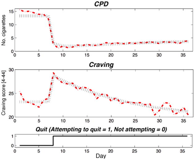
Averaged Craving and CPD ILD (dash-dot red) used to model Craving-mediated changes in CPD during a quit attempt; model predictions depicted as dotted brown lines.
| (11) |
As indicated by the quit attempt simulated using these models (dotted brown in Fig. 3) and the 64.7% fit for Craving and 84.38% fit for CPD, these models quantify the mediational relationship hypothesized to be at play within smoking cessation behavior change. Examining these equations suggest the direct X(t) → Y(t) path models the immediate reduction in CPD that occurs on TQD, while the X(t) → M(t) → Y(t) path—i.e., Pa and Pb in series— models the small and slow resumption of smoking post-TQD. The parameter estimates also reflect the inverse response in Craving (initial increase before ultimately settling to reduced levels, reflected in the negative Pa gain and zero term values), the fast reduction in smoking on TQD (there are no time constants or derivative terms required by Pc′), and the small resumption in smoking (small Pb gain, equal to -0.30) [5].
IV. Summary & Future Work
The case studies presented in this paper illustrate the potential of a dynamical systems approach for describing theorized behavior change mechanisms. Specifically, stemming from a connection between production-inventory management in supply chains [4], [9], differential equation models were presented that leverage ILD to describe behavior change according to SCT and mediational processes in the context of a physical activity intervention and smoking cessation. While promising, both of the case studies presented entail secondary analysis of existing data, which were not obtained through experiments designed with dynamical systems modeling in mind. In the future, high fidelity models with greater predictive ability could be estimated using more informative data collected through novel trials that are better suited for this analytical approach. Notably, experiment-design principles from system identification could be used to develop novel input signals [1], [4]. For these experiments, the value of the adjustable input signal of interest would be varied over time such that the input signal is more persistently excited in order to promote a greater range of dynamics and variability in the outputs [7]. As the processes examined in these experiments involve human subjects, these protocols must adhere to strict practical, ethical, and medical constraints. For example, [4] describes a “patient-friendly” clinical trial protocol which varies the dose of a pharmaceutical for a pain-management intervention on a biweekly basis, and repeats the dose schedule so that the first set of measurements can be used for estimation and the second set for validation. Ultimately, more rigorous estimation and validation of dynamical systems models should draw from data obtained in such novel clinical trials in order to more reliably quantify the dynamics of SCT and mediational processes.
Footnotes
This work was supported by the Office of Behavioral and Social Sciences Research and the National Institute on Drug Abuse at the National Institutes of Health through grants k25 da021173, r21 da024266, and f31 da035035.
Contributor Information
Kevin P. Timms, Email: ktimms@asu.edu.
César A. Martín, Email: cmartinm@asu.edu.
Daniel E. Rivera, Email: daniel.rivera@asu.edu.
Eric B. Hekler, Email: eric.hekler@asu.edu.
William Riley, Email: william.riley@nih.gov.
References
- 1.Martín CA, Rivera DE, Riley WT, Hekler EB, Bunam MP, Adams MA, King AC. A dynamical systems model of Social Cognitive Theory. Proceedings of the 2014 American Control Conference, pages. 2014:2407–2412. [Google Scholar]
- 2.Collins LM. Analysis of longitudinal data: The integration of theoretical model, temporal design, and statistical model. Annual Review of Pscychology. 2006;57(1):505–528. doi: 10.1146/annurev.psych.57.102904.190146. [DOI] [PubMed] [Google Scholar]
- 3.Walls TA, Schafer JL, editors. Models for Intensive Longitudinal Data. Oxford University Press; Cary, NC, USA: 2006. [Google Scholar]
- 4.Rivera DE. Optimized behavioral interventions: What does system identification and control systems engineering have to offer? Proceedings of the 16th IFAC Symposium on System Identification, Brussels, Belgium, pages. 2012 Jul;:882–893. [Google Scholar]
- 5.Timms KP, Rivera DE, Collins LM, Piper ME. Continuous-time system identification of a smoking cessation intervention. International Journal of Control. 2014;87(7):1423–1437. doi: 10.1080/00207179.2013.874080. [DOI] [PMC free article] [PubMed] [Google Scholar]
- 6.Ogunnaike B, Ray W. Process dynamics, Modeling, and Control. Oxford University Press; New York City, NY: 1994. [Google Scholar]
- 7.Ljung L. System Identification: Theory for the User. 2nd. Prentice-Hall, Inc.; Englewood Cliffs, NJ: 1999. [Google Scholar]
- 8.Ljung L. System Identification Toolbox User's Guide. The Math-Works, Inc.; 2003. [Google Scholar]
- 9.Nandola NN, Rivera DE. An improved formulation of Hybrid Model Predictive Control with application to production-inventory systems. IEEE Transactions on Control Systems Technology. 2013;21(1):121–135. doi: 10.1109/TCST.2011.2177525. [DOI] [PMC free article] [PubMed] [Google Scholar]
- 10.Bandura A. Social foundations of thought and action: a social cognitive theory. Prentice-Hall, Inc.; 1986. [Google Scholar]
- 11.MacKinnon D. Introduction to Statistical Mediation Analysis. Rout-ledge Academic; 2008. [Google Scholar]
- 12.King AC, Hekler EB, Grieco LA, Winter SJ, Sheats JL, Buman MP, Banerjee B, Robinson TN, Cirimele J. Harnessing different motivational frames via mobile phones to promote daily physical activity and reduce sedentary behavior in aging adults. PLOS One. 2013:e62613. doi: 10.1371/journal.pone.0062613. [DOI] [PMC free article] [PubMed] [Google Scholar]
- 13.McCarthy DE, Piasecki TM, Lawrence DL, Jorenby DE, Shiffman S, Fiore MC, Baker TB. A randomized controlled clinical trial of bupropion SR and individual smoking cessation counseling. Nicotine and Tobacco Research. 2008;10(4):717–729. doi: 10.1080/14622200801968343. [DOI] [PubMed] [Google Scholar]