Registration of whole immunohistochemical slide images: an efficient way to characterize biomarker colocalization

Abstract

Background and objective Extracting accurate information from complex biological processes involved in diseases, such as cancers, requires the simultaneous targeting of multiple proteins and locating their respective expression in tissue samples. This information can be collected by imaging and registering adjacent sections from the same tissue sample and stained by immunohistochemistry (IHC). Registration accuracy should be on the scale of a few cells to enable protein colocalization to be assessed.

Methods We propose a simple and efficient method based on the open-source elastix framework to register virtual slides of adjacent sections from the same tissue sample. We characterize registration accuracies for different types of tissue and IHC staining.

Results Our results indicate that this technique is suitable for the evaluation of the colocalization of biomarkers on the scale of a few cells. We also show that using this technique in conjunction with a sequential IHC labeling and erasing technique offers improved registration accuracies.

Discussion Brightfield IHC enables to address the problem of large series of tissue samples, which are usually required in clinical research. However, this approach, which is simple at the tissue processing level, requires challenging image analysis processes, such as accurate registration, to view and extract the protein colocalization information.

Conclusions The method proposed in this work enables accurate registration (on the scale of a few cells) of virtual slides of adjacent tissue sections on which the expression of different proteins is evidenced by standard IHC. Furthermore, combining our method with a sequential labeling and erasing technique enables cell-scale colocalization.

INTRODUCTION

Whole-slide imaging is an essential tool for digital pathology in which glass slides are digitized into virtual slides (VSs). Digital pathology permits the gathering and sharing of information for medical education, diagnosis, and research.¹ One particular research field in digital pathology is concerned with tissue-based biomarkers that are indicative of a normal or abnormal process (or of a condition or disease) and can be used for diagnostic, prognostic, and therapeutic purposes. These biomarkers can target the morphology and architecture of cells or tissues as well as gene and protein expression, which can be evidenced in tissue samples by using certain staining techniques, such as in-situ hybridization (ISH) and immunohistochemistry (IHC).^1–3

Multiple proteins must be simultaneously examined to extract relevant information from the complex biological processes involved in serious pathologies such as cancers. The colocalization of protein expression that can be revealed by IHC in formalin-fixed paraffin-embedded (FFPE) tissue samples yields detailed information related to the potential protein interaction to be extracted. This type of information produces both morphologic information and molecular and functional information, potentially increasing the specificity and/or sensitivity of the resulting indicators in terms of their diagnostic, prognostic, or theragnostic value. Different approaches were developed to allow the colocalization of two or more biomarkers in FFPE or frozen tissue sections. Most of the approaches use fluorescence labeling with frozen sections,^4–8 and comparatively few use brightfield IHC with FFPE tissue sections.^9–12 However, the latter approach is easier to implement and offers better preservation of the tissue morphology. Fluorescence-based labeling does have certain advantages in colocalizing antigens (eg, its ability to both multilabel and detect individual labels), but it features several disadvantages in practice (eg, the need for frozen tissue slices, labeling fading, tissue autofluorescence, cost of the imaging equipment, etc.). Consequently, brightfield IHC staining on FFPE tissue sections is more suited for the high-throughput tissue sample processing involved both in clinical research and in the daily routine of hospital pathology departments.

Brightfield multichromogenic methods for multiple antigen labeling, in which each biomarker is evidenced by a different color, are limited and have had many challenges over the years.^13–16 The essential problems result from antibody cross-reactions and interpretation difficulties. These latter occur if different targeted proteins are expressed in the same cellular compartment (eg, the cell nuclei), then color merging or masking arises. As an alternative method, biomarker colocalization can be determined by cutting adjacent (or serial) tissue sections ranging in thickness from 3 to 5 μm, submitting each section to standard IHC, digitizing the slides, and finally registering the adjacent VSs. Because the slides are thinner than the average size of human cells, pluricellular structures such as glands or epithelium are often well preserved across several slides. Thus, analyzing adjacent slides enables the colocalization of protein expression at a histological level; however, it also requires a more complicated image analysis processes, such as the accurate registration of VSs for viewing and extracting the colocalization information.^12,17,18

An interesting alternative to multichromogenic IHC was recently proposed by Glass et al.¹⁹ who described a method to label the same tissue slide multiple times using brightfield IHC. This ‘sequential immunoperoxidase labeling and erasing’ (SIMPLE) method requires the creation of a VS after each labeling. After digitization, the staining is erased (or washed) and a new cycle of staining–digitization–erasing can be performed. Staining erasing is a difficult technique that uses an antibody elution technique intended to preserve tissue and antigen epitopes for the next staining. By correcting certain parameters and including a new elution methodology, we recently improved the SIMPLE methodology and successfully utilized it with antigens expressed in the same cellular compartment (unpublished data). Figure 1A compares the workflows of our SIMPLE-like method to the standard IHC procedure applied to serial slides.

Figure 1:

(A) Sequence of steps involved in our SIMPLE-like method compared to the standard serial slide staining procedure. (B) Illustration of the annotation process on serial slides. For each group of four slides, a reference slide in the center of the stack was chosen (ie, FHL-2). On the reference slide, five ROIs were distributed and the pathologist annotated six CPs and six SCs in each ROI. Then, she selected the corresponding CPs and SCs on the three other slides of the stack by matching them with the reference slide. CP, control point; ROI, regions of interest; SIMPLE, sequential immunoperoxidase labeling and erasing.

The registration of VSs thus becomes an essential step for the colocalization of IHC biomarkers with the serial slides or the SIMPLE-like method. It is a relatively new problem that presents different challenges than those traditionally encountered in the registration of digital radiology images.¹⁷ The most important of these challenges is the size of the images: VSs are typically 30 000 pixels in height by 60 000 pixels in width, which is approximately 2 × 10⁹ pixels in total. In addition, this method differs from multimodal digital radiology images where different modalities applied to the same region are registered; in the case of serial slides, we need to register different but adjacent slides that were independently processed to evidence different biomarkers by IHC. The IHC staining pattern depends on the targeted antigen and its cellular location and can possibly yield large variations in pixel intensity between adjacent VSs. It should also be noted that the tissue process may introduce non-linear deformations such as tearing, shearing, folding, and shrinking.

Although VS registration is a relatively new problem, the registration of small histological images (HIs) is a well-studied field of research. These images show either the entire tissue with a lower resolution or a small section of the tissue with a higher resolution. Three-dimensional (3D) volume reconstruction is also often addressed in this context,^20–28 as it requires sequentially registering pairs of two-dimensional (2D) HIs and propagating the registrations to realign all the images of the stack.^25,26,28 To avoid error propagation, some authors proposed the introduction of constraints related to the 3D nature of their dataset.^21,23,27,29

In contrast, the problem of registering multiple HIs to measure the overlap or colocalization of multiple IHC biomarkers is addressed much less in the literature (and even less for complete VSs). Often, colocalization was manually and qualitatively evaluated by viewing the same histological region in different slides and showing the different pictures side by side.^10,30,31 Rademakers et al.¹⁸ used an interactive ‘register’ function in IPLab (Scanalytics) that could rotate and shift images to manually register VS pairs to assess the colocalization of two IHC biomarkers on adjacent tissue sections from biopsies.

To the best of our knowledge, all of the methods studying full-sized VSs used a pyramidal registration technique that first registered a downsampled version of the image and then refined the registration result by initializing new registration steps with incrementally increasing resolutions. For example, Cooper et al.thinsp;³² applied an automatic two-step procedure to register H&E- and IHC-stained slides of mouse mammary glands and of follicular lymphomas.³³ The first step in the procedure was a rigid registration that was guided by matching pairs of histological structures. The second step was a non-rigid transformation that was guided by matching either image patches³² or a subset of histological structures.³³

In Mueller et al.¹⁷ the authors tackle the problem of visualizing two or more VSs, which enables the visualization of an H&E slide together with an IHC-stained slide that shows a prognostic biomarker. The challenge was to provide an almost-real-time registration so that two slides could be easily viewed at the same time. They also proposed a two-step approach based on the open-source program elastix, originally developed to register in vivo images.³⁴ The first step in the approach was a global pre-registration step that was performed offline prior to viewing. A second, online transformation was then instantly applied to each field of view (FOV) requested by the pathologist during his/her navigation throughout the VSs. The registration error was computed on five regions of interest (ROIs), only for the offline step, each ROI containing 10 point-based landmarks. The results had a maximal registration error of 130 μm after the offline registration stage.

Finally, Metzger et al.¹² also used a two-step registration method to analyze H&E- and IHC-stained slides scanned at 20 × magnification. This method combines a coarse manual alignment with an automatic fine registration using a software module called TurboReg, which uses a pyramid approach initially proposed for the registration of positron emission tomography and fMRI images.³⁵ During the first step, manual manipulations were used to flip and rotate three adjacent IHC VSs so that they were in rough alignment with a reference H&E VS. The TurboReg software then automatically completed the registration process through rigid transformations, though affine transformations were also available. However, the results displayed relatively high registration errors: they were computed on 150 landmark pairs distributed across the H&E and IHC VSs and had median errors of 88–114 μm (depending on the stains) and a maximal error of 398 μm. Note that the cell diameter of the tissue under analysis (prostate cancer) is in the range 15–20 μm.

The present study aims to provide an accurate image registration technique that applies to high resolutions (typically equivalent to 20 × magnification) and is motivated by the need to perform valid biomarker colocalization analyses. This need requires registration accuracy on the scale of a few cells. To this end, a two-step registration strategy where a global low-resolution registration initializes the registrations of separate FOVs seems appropriate. The independent registration of FOVs increases the registration accuracy by locally reducing alignment errors. However, this technique requires as many additional registrations as the number of independent FOVs. Therefore, a fast registration method is essential. In addition to the performance in terms of accuracy and speed, the accurate analysis of biomarker colocalization necessitates the preservation of pixel size in the VSs (and FOVs) after transformation. Considering all of these reasons, we decided to extend the work presented in Mueller et al.¹⁷ which demonstrated fast and promising results. We use parametric transformations that preserve the shape and dimension of the pixels, and we characterize the registration errors on high-resolution FOVs for different types of tissue by imaging serial IHC slides as well as slides that have been stained multiple times with IHC (using our SIMPLE-like procedure).

MATERIALS

All the slides in the study were scanned at 20 × magnification (NanoZoomer HT 2.0, Hamamatsu, Hamamatsu City, Japan) and annotated by a pathologist by means of NDP.view (Hamamatsu). The first dataset, referred to as SERIAL, consisted of eight groups of four serial slides (4 μm thick) from colorectal cancer samples. For each group, the first slide was stained with E-cadherin, the second with FHL-2 (four-and-a-half LIM domains protein 2), the third with B-catenin, and the fourth with vimentine (Vim) (see figure 1B). For each group, we selected five ROIs on the FHL-2 VS, which was chosen as the reference for the annotations because of its central location within the stack of slides. For each ROI of the FHL-2 VS, a pathologist placed six control points (CPs) at remarkable loci and segmented six histological structures, totaling 30 CPs and 30 segmented contours (SCs) per slide. The pathologist manually matched the CPs and SCs on the other VSs of the stack to constitute the complete supervised dataset made of 24 pairs of annotated slides.

We also constructed a second dataset made of six pairs of VSs consisting of six tissue slides from tonsil and brain tissue samples, each sequentially stained to identify two different IHC markers using our SIMPLE-like technique (see Introduction). The sequential pairs of IHC markers targeted membranous CD3 and CD20 expression, cytoplasmic glial fibrillary acidic protein (GFAP) and Vim expression, and nuclear p53 and Ki67 expression. The VS marked with the first biomarker of each pair (ie, CD3, CD20, P53, Ki67, GFAP, or Vim) was used as reference to distribute five ROIs. Similar to the SERIAL dataset, a pathologist manually annotated six CPs and six SCs for each ROI and matched them on the VS with the second biomarker (CD20, CD3, Ki67, P53, Vim, or GFAP, respectively).

Finally, we constituted an independent dataset, referred to as TEST, for validation purposes. The TEST dataset was made of seven groups of two serial slides (targeting Ki67 and epidermal growth factor receptor, respectively) of high-grade glioma tissue samples. For each VS a pathologist manually annotated CPs in five ROIs (six CPs per ROI).

METHODS

Because the method presented in Mueller et al.¹⁷ had a nearly real-time registration performance and was efficiently applied to various IHC-stained VSs, we were motivated to further investigate the possibility of using the elastix framework to identify biomarker colocalization. The different components of the registration available for customization in this framework are presented in figure 2 and detailed below.

Figure 2:

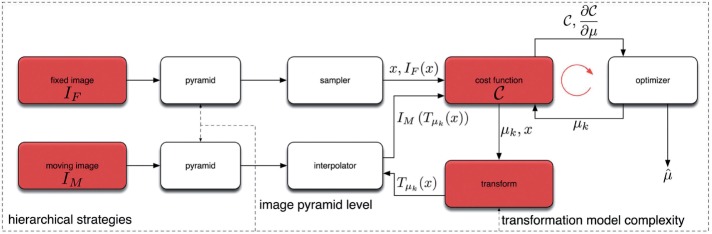
Basic registration components of the elastix framework (adapted from Klein et al.³⁴). At each registration step (low- or high-resolution), a pyramidal registration procedure optimizes the parameters (μ_k) of the transformation (T_μ) to minimize the value of the cost function (C). Our benchmark application tests different combinations of the elements in red (see details in the main text).

The two steps in our registration strategy use the elastix framework, in which the input images are selected with increasing resolution levels (ie, a pyramidal registration approach). To register VSs labeled with different antibodies, we chose the luminance image as the input for the low-resolution step. We tested various color transformations as the input for the high-resolution step. The executable and the C ++ code of elastix are available on the elastix website (http://elastix.isi.uu.nl).

The resolution levels are controlled by the ‘pyramid’ component that reduces the images by several factors using Gaussian-like downsampling.³⁶ The result is a (Gaussian) pyramid from which the full-resolution image constitutes the base level (level 0), and the lowest-resolution image corresponds to the highest level of the pyramid. All the experiments related to the global low-resolution registration step were conducted using a Gaussian pyramid with four levels corresponding to the following magnifications: 0.125 × , 0.25 × , 0.5 × , and 1 × . For the experiments related to the local, high-resolution registration steps, we also chose a Gaussian pyramid with four levels, but the corresponding magnifications were 2.5 × , 5 × , 10 × , and 20 × (needed for the biomarker colocalization analysis).

The interpolator component of elastix computes the pixel values of the moving image at the locations that correspond to the pixels of the fixed image. This correspondence is established by means of a parametrized transform (T_μ), which must be optimized. In Mueller et al.¹⁷ the authors used a B-spline transform as the first, deformable transformation. Although it seemed to provide a satisfactory result for the simultaneous viewing of two slides, optimizing the parameters of this first transformation is computationally demanding. Furthermore, we observed strong distortions, such as wraps, on our VSs that are not desirable for biomarker colocalization analysis. Therefore, we modified the method presented in Mueller et al.¹⁷ and tested the possibility of using only linear transformations (affine and Euler transforms) for both registration steps.

The values of the corresponding pixels in the fixed and moving images are used to determine the value of a similarity function, S. For the low-resolution registration step based on the luminance images (which are impacted by the different stains), we chose Mattes’ mutual information (MI) as the similarity function S because it is one of the most popular image similarity measures for the registration of multimodality images.³⁷ In contrast, the registration of images in the same modality can be considered for higher-resolution images after color deconvolution. Indeed, by using the method detailed in Ruifrok et al.³⁸ we are able to separate the brown staining (DAB, i.e. 3, 3′-diaminobenzidine) from the hematoxylin (blue) counter-staining and to use the hematoxylin channel (hem) for the registration of the high-resolution FOVs. These findings led us to also test the normalized cross-correlation (NCC) as function S, which assumes an affine relation between the pixel intensity values of the two images.³⁴

The optimizer component is a stochastic gradient descent (SGD) method that searches the linear transformation parameters (μ_k) to minimize the cost function C = −S. We also investigated the convergence speed for the different combinations of input image types and cost functions by testing different numbers of iterations (1000 or 2000) as well as the maximum step lengths (25, 50, 75, 100, 125, 150, or 300) for each optimization stage. In the end, the transformation parameters μ_k are modified according to the optimization result. The newly parametrized transformation serves as the initialization of the next optimization stage, using the images at the following level of the pyramid, which have a higher resolution.

To increase the registration speed and robustness (by avoiding local minima³⁷), C is not evaluated on the complete images but on randomly sampled pixels; we also tested the number of randomly sampled pixels in our benchmark (2500, 4000, 5000, 7500, 9000, or 10 000). The randomization and retrieval of the pixel values is made by the sampler in a fixed image or by the interpolator in a moving image. For the experiments conducted in this work, we chose a B-spline interpolator.³⁴

For each parameter set (PS)—which consisted of the values provided to the elastix framework in terms of the number of iterations, the maximum step length and the number of sampled pixels used to evaluate C—we evaluated the low-resolution registration accuracies using the root mean square error (RMSE) computed on the CPs. For the high-resolution step, the PS also included the color transformation (luminance or hem channel) and similarity function S (MI or NCC). For high resolutions, we also computed the Hausdorff distance (HD) on the SCs (see the Materials section).

To identify the best PSs, we compared the RMSE (and HD) values that were computed before (RMSE-O, HD-O) and after the registration (RMSE-R, HD-R) using the T statistic from the Wilcoxon matched-pair test provided in the Statistica package (StatSoft, Tulsa, Oklahoma, USA). If the registration procedure is efficient, a large majority of the differences of the RMSE (and HD) values before and after registration should be negative, which would lead to a small T value (T = 0 indicates that all differences have the same sign).³⁹ For the low-resolution registration step we also computed RMSE values provided by TurboReg, a method previously used to register images of IHC-stained slides.¹² It should be noted that TurboReg uses the Levenberg–Marquardt optimization method to minimize the squared difference of pixel intensities.³⁵

To determine the quality of the best results provided by elastix, we compared them with those obtained using the supervised (rigid or affine) registrations based on the CP pairs. To this end, we used the CorrespondingPointsEuclideanDistanceMetric included in elastix. This supervised registration approach can be viewed as providing an optimal RMSE reference, but is not practical because it requires an expert to locate (as exactly as possible) several CP pairs for each FOV to be registered.

The elastix PSs selected on the basis of the SERIAL dataset were applied to the TEST set. The fully commented parameter files required by elastix are provided in the online supplementary material.

RESULTS

We benchmarked the combinations of the elastix components (shown in red in figure 2) on the two datasets (SERIAL and SIMPLE) and for two different resolution steps (low resolution: 1 × , high resolution: 20 × ). We first present the results on the SERIAL dataset, which is an example of the most general situation for biomarker analysis on VSs acquired from serial IHC slides. The low-resolution registration results are presented first, with the goal of finding a combination of the elastix components that enables the robust optimization of the linear transformation parameters (μ_k). We then present the high-resolution registration results that are obtained after initialization by the low-resolution step. Finally, the results of the benchmarks conducted on the SIMPLE dataset, which illustrates an improved situation for biomarker analysis in which multiple VSs are acquired from the same tissue section, are presented.

To illustrate the differences between these two IHC approaches (SERIAL vs SIMPLE), we computed the RMSE of the original conditions before any registration (RMSE-O) for the 30 CPs for each image pair. To register the SIMPLE-like VSs, we register the same tissue slide that is stained twice (including an elution step to remove the first staining). Thus, it is not surprising that we observed strongly lower RMSE-O values for the SIMPLE dataset compared to the SERIAL dataset (see figures 3A and 4A).

Figure 3:

Box plots of the RMSE and HD values (in μm) for the original conditions (RMSE-O and HD-O) and for those obtained after registration with the parameter sets (PSs) used in the low- (A) and high-resolution (B and C) steps for the SERIAL set. The boxes show the IQRs, and the medians are shown as thin lines in each box. The whiskers show the non-outlier ranges, and the outliers are drawn with the ‘ + ’ symbol. (A) RMSE-O and RMSE-R values obtained with the 30 low-resolution PSs identified by applying condition (1). The continuous horizontal line shows the 60-μm limit to compare with percentiles 75. (B) RMSE-O and RMSE-R values obtained with the seven high-resolution PSs identified by applying condition (2). The original condition for the high-resolution registration step is the result of the low-resolution step (ie, PS19 in A). The horizontal lines show the 20- and 31-μm limits that approximately correspond to percentile 25 of the RMSE-O and to the maximum RMSE-R value encountered, respectively. (C) HD-O and HD-R values obtained with the seven PSs in B. The horizontal line shows the median HD-O value (249 μm). HD, Hausdorff distance; RMSE, root mean square error; IQR, interquartile range.

Figure 4:

Box plot of the RMSE-O and RMSE-R values (in μm) obtained with the parameter sets (PSs) used in the low- and high-resolution registration steps for the SIMPLE set. The boxes show the IQRs, and the medians are shown as thin lines in each box. The whiskers show the non-outlier ranges and the outliers are drawn with the ‘ + ’ symbol. (A) RMSE-O and RMSE-R values obtained with the 24 low-resolution PSs, completed using the 12 additional PSs (PS25 to PS36) tested with smaller N_s values (see main text). The continuous horizontal line shows the 20-μm limit. (B) RMSE-O and RMSE-R values obtained with the seven high-resolution PSs exhibiting, at most, two FOVs with RMSE-R values higher than the RMSE-O values. The continuous horizontal line shows the 5-μm limit (see main text for details). FOV, field of view; RMSE, root mean square error; SIMPLE, sequential immunoperoxidase labeling and erasing; IQR, interquartile range.

Low-resolution step on serial VSs

During the low-resolution registration step, we tested both affine and rigid transformations that were optimized with MI as the similarity function S. The value of S was estimated using N_s pixels sampled from the luminance of the equivalent 1 × magnification images. The number of iterations, N_i, of the SGD optimization procedure is fixed, so there is no early stop, and the maximum displacement (in pixels) allowed at each iteration is given by the maximum step length (MSL). The tested values of the parameters of the optimization procedure are listed in table 1. Additionally to these tests with elastix, we also applied TurboReg with parameters similar to those used in Metzger et al.¹² that is, a rigid transformation with the luminance image used as input.

Table 1:

Tested values for the parameters of the stochastic gradient descent optimization procedure for the low- and high-resolution steps applied on the SERIAL dataset

Parameter	Low-resolution	High-resolution
Tμ	Affine, rigid	Affine, rigid
S	MI	MI, NCC
Ns	2500, 4000, 5000, 7500, 9000, 10 000	8000
Ni	1000, 2000	2000
MSL	25, 50, 75, 100, 125, 150, 300	5, 25, 50, 100
Input	lum	lum, hem

T_μ is the parametric transformation model. S is the similarity function. N_s is the number of samples (ie, pixels) used to estimate the value of S. N_i is the number of iterations of the procedure. MSL is the maximum displacement (in pixels) allowed at each iteration. Input indicates the input image (lum = luminance image, hem = hematoxylin channel) resulting from the color deconvolution.

MI, mutual information; MSL, maximum step length; NCC, normalized cross-correlation.

For each of the resulting 168 PSs, we compared the RMSE values computed from the 30 CPs after the equivalent 1 × magnification images of the entire slides were registered. All PSs provided a large majority of RMSE-R values that were lower than the RMSE-O values. We then used the T statistic of the Wilcoxon matched-pair test to filter out the best performing combinations. We isolated 30 PSs for which all but one of the 24 differences (RMSE-R − RMSE-O) are negative and for which the rank of the sole positive difference is either 1 or 2 (ie, among the smallest values; see online supplementary table S1) by applying the following selection condition:

1

The RMSE-R value distributions obtained with these PSs are shown in figure 3A, and the corresponding parameter values are detailed in online supplementary table S1. It should be noted that TurboReg did not satisfy condition (1) because it provided a T value of 25 (with a p75_RMSE of 124 μm), that is, the fifth highest T value among all the tested PSs of elastix.

A rigid transformation was included only for PS1, PS2, and PS3, all of which exhibited relatively high RMSE-R values (see online supplementary table S1). In contrast, 75% of the registrations made with PS19, PS25, and PS30 had RMSE-R values smaller than 60 μm, whereas the RMSE-O values had a median of 1299 μm (see online supplementary table S1). The latter three PSs used an affine transformation with at least 7500 pixels (N_s) to estimate S and an MSL of either 100 or 150 pixels (ie, 920 μm or 1380 μm). From these three equivalent PSs, we chose PS19 to initialize the upcoming high-resolution registration step because it is the least computationally expensive (N_s = 7500 and N_i = 1000).

High-resolution step on serial VSs

During the high-resolution registration step, we once again tested affine and rigid transforms that were optimized using either MI or NCC as the similarity function S. In light of the good optimization results obtained from the low-resolution step, we chose N_s = 8000 pixels to evaluate S and the number of iterations N_i = 2000 for the SGD optimization procedure. The value of S was thus estimated from 8000 pixels sampled from either the luminance (lum) or the hematoxylin channel (hem) of the equivalent 20 × magnification of each FOV. The maximum displacement (in pixels) allowed at each iteration is given by the MSL (see table 1).

For each of the 32 PSs, we compared the RMSE and HD values obtained for each FOV after registration. The RMSE values were computed on the six CPs, while the HD values were computed on the six SCs, but both sets were computed after the registration of the equivalent 20 × magnification images of the FOVs. Again, we used the T statistic to determine the best-performing combinations with respect to the RMSE (T_RMSE) and HD (T_HD). We used the following selection condition to isolate seven PSs (see online supplementary table S2) for which at most 11 out of 95 FOVs exhibited RMSE-R (HD-R) values larger than the RMSE-O (HD-O) values:

2

Compared to the low-resolution step, a higher RMSE threshold value was used both because the T statistic was evaluated for 95 pairs (in place of 24 at low resolution) and because the low-resolution step used as initialization already provided low RMSE-O (and HD-O) values (cf. figure 3B, C). Interestingly, online supplementary table S2 shows that all of these PSs used NCC as the similarity function S, regardless of the input. In addition, five out of seven PSs used a rigid transform, supporting the findings of Mueller et al.¹⁷ that a simple transformation produces high accuracy at high resolutions. Overall, the best performances were provided by PS5 (see online supplementary table S2, figure 3B, C), although it failed to correctly register an FOV showing a tissue fold (see figure 5A, B) that was the largest outlier in figure 3B, C. This result illustrates the impact that a tissue defect may have on the registration results. In the discussion section, we suggest methods to identify registration errors on specific FOVs to omit them from subsequent analyses (or to manually correct it, if it is absolutely required).

Figure 5:

Illustration of two pairs of FOVs (seen at 8 × equivalent magnification) registered using PS5. The first column (A and C) shows the FOVs used as the fixed images as blue rectangles. Six control points (CPs) and six manually segmented contours (SCs) per image are also shown in blue. The second column (B and D) shows the corresponding FOVs used as the moving images (identified by the low-resolution registration step) as red quadrilaterals and where the green CPs and SCs (corresponding to those in A or C) were manually defined by a pathologist (‘ground truth’). The registration is initialized with the low-resolution step, transforming the blue CPs and SCs of the image from the first column (A or C) to those shown in black in the second column (B or D). A subsequent high-resolution registration step is then applied by using PS5, resulting in the red CPs and SCs. The RMSE (HD) values were calculated between the green and red CPs (SCs). The first row (A and B) shows an incorrect FOV registration for which the final RMSE (HD) value was 226 μm (887 μm). The second row (C and D) shows a successful FOV registration for which the final RMSE (HD) value was 17 μm (119 μm). FOV, field of view; HD, Hausdorff distance; RMSE, root mean square error.

To provide an optimal but realistic reference, we also applied supervised registrations that use the CP pairs to optimize the rigid and affine transformations. The results obtained from these two optimal registrations were very similar and, comparatively, our completely unsupervised method using PS5 provides very satisfactory results (see online supplementary figure S1 and figure 5C, D).

Low-resolution step on the SIMPLE-like VSs

The results obtained from the SERIAL dataset show that affine transforms are preferable for low-resolution registrations, that N_s should be sufficiently large (greater than 5000), and that serial VSs are registered appropriately with N_i = 1000. However, as mentioned above, SIMPLE-like VSs are easier to register than serial VSs, so we used smaller values of the MSL parameter in these tests (see table 2).

Table 2:

Tested values for the parameters of the stochastic gradient descent optimization procedure for the low- and high-resolution steps for the SIMPLE dataset

Parameter	Low-resolution	High-resolution
Tμ	Affine	Rigid
S	MI	MI, NCC
Ns	5000, 7500, 9000, 10 000	8000
Ni	1000	2000
MSL	1, 5, 10, 20, 30, 40	1, 5, 25, 50
Input	lum	lum, hem

See table 1 for the meaning of the parameters.

MI, mutual information; MSL, maximum step length; NCC, normalized cross-correlation; SIMPLE, sequential immunoperoxidase labeling and erasing.

For all the tested PSs (listed in online supplementary table S3) and all the registered image pairs, the RMSE-R values were significantly smaller than the RMSE-O values (see figure 4A). Consequently, the T statistic was equal to zero for each PS. Interestingly, online supplementary table S3 shows a dramatic increase in RMSE-R for MSL values above 10 (except for PS4), and this effect increases with the value of N_s. Thus, we also tested smaller values of N_s, N_s = 2500 (PS25 to PS30), and N_s = 4000 (PS32 to PS36) in addition to the six MSL values detailed in table 2. We observed the same negative impact of large MSL values on the results, but the effect was reduced due to the smaller N_s (see figure 4A, where PS25 to PS36 are shown first for illustration purposes). All PSs with MSL≤10 have a maximal RMSE-R value of 19 μm, which is approximately two pixels on the equivalent 1 × magnification image used in the low-resolution registration step.

In conclusion, we chose PS27 with N_s = 2500 (faster computation time) and MSL = 10 to initialize the following high-resolution registration step.

High-resolution step on the SIMPLE-like VSs

The results on serial VSs show that rigid transformations offer good accuracy at high resolutions. Therefore, we only tested rigid transformation models for the high-resolution registration step on the SIMPLE dataset. The transformation models were optimized using either MI or NCC as the similarity function S, which was evaluated using either the lum or the hem channel of the equivalent 20 × magnification of each FOV. We also used the same values for N_s (8000 pixels) and N_i (2000) as on serial VSs. The tested values for MSL are listed in table 2.

Figure 4B shows seven of the 16 PSs tested with the 30 different FOVs (listed in online supplementary table S4); these seven were selected (in bold in online supplementary table S4) because they exhibited at most two FOVs for which the RMSE-R (HD-R) value was larger than the RMSE-O (HD-O) value. As shown in online supplementary table S4, six of these PSs used NCC as the similarity function S, even when registering the luminance images. In fact, we observed that the input image had less impact on the registration accuracy than the MSL parameter (see online supplementary table S4 and figure 4B). With the SIMPLE VSs, PS7 performed better than all other PSs and all registered FOV pairs exhibited RMSE-R values smaller than 5 μm.

Even after an accurate low-resolution registration step, the high-resolution registration step remained useful and provided significantly better registration, as illustrated by the T statistic values reported in online supplementary table S4 (associated with p values <10⁻⁴). Figure 4B confirms that all of the FOVs registered with PS7 exhibited RMSE-R values below 5 μm, which is approximately the diameter of a cell nucleus in the tissue samples.

Application of the PSs selected for serial slides on the TEST VSs

We registered the TEST VSs by successively applying the low- and high-resolution steps with the PSs giving accurate results on the SERIAL dataset (see result sections above). We characterized the registration accuracy by using the control points placed manually by a pathologist and computing the RMSE values after the low (RMSE-RL) and high-resolution (RMSE-RH) registration steps. It should be noted that the brain tumor samples constituting the TEST dataset presented very few histological structures. The VSs were thus less textured and more difficult to register, especially for the high-resolution step, compared with the colonic tissue samples constituting the SERIAL dataset.

For the 35 ROIs constituting the TEST dataset, we obtained relatively large RMSE-RL values after the low-resolution registration step using PS19. While on the SERIAL dataset 75% of the RMSE-RL values were below 42 μm and the maximum value was 97 μm, on the TEST set 75% of these values were above 40 μm and the maximum value was 246 μm. However, this maximum corresponds to a shift of 25 pixels at low resolution, that is, about 1% only of the width of the image (2438 pixels). This low-resolution step was thus used to initialize the high-resolution one.

As expected, the lack of histological structures more affected the high-resolution registration step. We tested different PSs from the seven selected in our previous experiment (see results above and online supplementary table S2), among which were similarly performing (PS4, PS5, and PS7) and less effective PSs (PS1 and PS2). We also tested these five PSs with an additional level in the downsampling pyramid, resulting in a total of 10 tested PSs. From this short comparative study, the best results were obtained with PS4 and PS4′ (ie, PS4 with the additional level in the downsampling pyramid), giving p75_RMSE-RH values of 86 and 79 μm, respectively, as compared to 101 μm for PS5. These results show that smaller displacements are preferable (MSL = 50 for PS4 in place of 100 for PS5, see online supplementary table S2) when histological structures are lacking. Nevertheless, even on tissue samples that are hard to register, such as the brain tumor samples included in the TEST dataset, a rapid exploration of the parameters can lead to acceptable registration results with an accuracy level corresponding to about four cell diameters.

DISCUSSION AND CONCLUSIONS

In this work, we showed that high registration accuracies can be achieved with simple transformation models (affine and rigid), even when registering VSs in the presence of non-linear deformations. The registration accuracy achieved with our approach is suitable for biomarker colocalization analysis. Indeed, registration errors as low as 20 and 5 μm were frequently achieved for the SERIAL and SIMPLE datasets, respectively, which approximately correspond to the diameters of a tumor cell and a tumor cell nucleus, respectively. However, these low registration errors on serial slides can only be achieved if histological structures are present and conserved between adjacent slides (such as in colonic tissue), else the registration errors may increase as demonstrated on the TEST dataset. However, as shown with the SIMPLE dataset including brain tissue samples, high registration accuracy can be reached for tissue samples lacking in histological structures by using VSs stained using our SIMPLE-like method. This approach can still offer a good alternative to the more limited double-staining method (see Introduction).

Compared with the results presented in Mueller et al.¹⁷ our simpler, low-resolution registration step exhibits a comparable error in terms of the RMSE. In contrast, the high-resolution registration step cannot be directly compared because Mueller et al.¹⁷ estimated the high-resolution registration accuracy by using the Jaccard and Dice coefficients on binarized images. These coefficients must be regarded as relative measures for the comparison of different registration methods applied on the same FOV pair. However, these results show that, for magnifications higher than 10 × , simple transformations (ie, local translations) can perform almost as well as more complex, deformable transforms. This observation agrees with our results that showed that rigid transforms are indeed accurate at 20 × magnification. Compared with other frameworks, elastix provide a better registration than the TurboReg software used in Metzger et al.¹² which exhibited much larger registration errors. Indeed, on the SERIAL dataset TurboReg exhibited a median error of 70 μm at 1 × , as compared with 37 μm for our method. A median error above 88 μm obtained at 20 × magnification was reported for prostate tissue in Metzger et al.¹²

Colocalization measurements on registered VSs can be carried out by means of extensions of the colocalization indices usually used to characterize the degree of overlap between two channels in fluorescence microscopy images.⁴⁰ In fluorescence microscopy, no registration is required because images are acquired on the same sample with different wavelengths. The usual colocalization indices are overlap, Manders’ coefficients, and possible extensions (eg, using rank-based intensity weighting⁴¹). In the case of registered VSs, similar indices can be computed on tiles. The tile sizes must be determined in relation to the registration accuracy. At high resolution, colocalization on serial VSs can be reasonably measured by using squared tiles 80 μm in length because the corresponding cells in two registered FOVs can be considered to be approximately 20 μm apart. On registered SIMPLE-like VSs, this tile size can decrease to 20 μm or even be directly computed after the low-resolution registration step on tiles of 60–80 μm length in view of the good results already obtained at this step. Figure 6 illustrates how to compute colocalization indices based on local staining measurements (via staining area or intensity measurements, as usually employed for characterizing global IHC staining^31,42).

Figure 6:

Example of colocalization index map computation at high resolution. (A) FHL-2 high FOV (20 × magnification). (B) Corresponding (ie, result of the low-resolution registration step) E-cadherin FOV (20 × magnification), which provides a good starting point for the high-resolution registration. (C and D) Usual staining measurements, such as the Quick-Score (ie, mean DAB intensity) as illustrated here, are computed on each tile. FOV A is divided into squared tiles 80 μm in length, and the high-resolution transform is then used to compute the corresponding tiles in FOV B (note the slight rotation of the tiles). The RMSE-R after the high-resolution registration for this pair of FOVs was 17 μm. (E) The local contributions to a global colocalization index, such as the overlap coefficient as illustrated here, are computed on each tile. The value of the global overlap index (which is the sum of the tile contributions and takes values between 0 and 1) is 0.8784 for the two FOVs. FOV, field of view; RMSE, root mean square error.

The simplicity of the transformation models and the extremely parallel nature of the high-resolution registration step enable the use of the method on large-scale studies involving hundreds of patients. Such large-scale studies prevent the use of CPs or SCs to evaluate the quality of a registration because it would necessitate an enormous amount of annotation work. To be fully efficient, an unsupervised approach, such as the one proposed in the present study, needs a method to detect incorrect or suboptimal registrations by using only (unsupervised) information extracted from the images, such as the value of the similarity function S, which is indicative of image pair similarity. Our observations on S values obtained after registration indicate that certain threshold values could be determined (at low and high resolution) to identify cases with insufficient registration accuracy. These data should be confirmed on larger series of registered image pairs.

CONTRIBUTORS

Conceived the study objectives: IS, CD. Designed the methods and experiments: XML, PB, CD. Contributed materials: LV, A-LT, LL, IS. Performed the implementation and the experiments: XML, PB, Y-RVE. Analyzed the data: XML, CD. Wrote the paper: XML, CD.

FUNDING

This work was supported by the Télévie program of the ‘Fonds National de la Recherche Scientifique’ (FNRS, Brussels, Belgium), the Fonds Yvonne Boël (Brussels, Belgium), and the Fonds Erasme. The CMMI is supported by the European Regional Development Fund and the Walloon Region. CD is a Senior Research Associate with the FNRS.

COMPETING INTERESTS

None.

PROVENANCE AND PEER REVIEW

Not commissioned; externally peer reviewed.

REFERENCES

- 1.Kothari S, Phan JH, Stokes TH, et al. Pathology imaging informatics for quantitative analysis of whole-slide images. J Am Med Inform Assoc 2013;20:1099–108. [DOI] [PMC free article] [PubMed] [Google Scholar]
- 2.Hassan S, Ferrario C, Mamo A, et al. Tissue microarrays: emerging standard for biomarker validation. Curr Opin Biotechnol 2008;19:19–25. [DOI] [PubMed] [Google Scholar]
- 3.Smith NR, Womack C. A matrix approach to guide IHC-based tissue biomarker development in oncology drug discovery. J Pathol 2014;232:190–8. [DOI] [PubMed] [Google Scholar]
- 4.Böcker W, Moll R, Poremba C, et al. Common adult stem cells in the human breast give rise to glandular and myoepithelial cell lineages: a new cell biological concept. Lab Investig 2002;82:737–46. [DOI] [PubMed] [Google Scholar]
- 5.Brouns I, Van NL, Van Genechten J, et al. Triple immunofluorescence staining with antibodies raised in the same species to study the complex innervation pattern of intrapulmonary chemoreceptors. J Histochem Cytochem 2002;50:575–82. [DOI] [PubMed] [Google Scholar]
- 6.Uchihara T, Nakamura A, Nakayama H, et al. Triple immunofluorolabeling with two rabbit polyclonal antibodies and a mouse monoclonal antibody allowing three-dimensional analysis of cotton wool plaques in Alzheimer disease. J Histochem Cytochem 2003;51:1201–6. [DOI] [PubMed] [Google Scholar]
- 7.Clarke CL, Sandle J, Parry SC, et al. Cytokeratin 5/6 in normal human breast: lack of evidence for a stem cell phenotype. J Pathol 2004;204:147–52. [DOI] [PubMed] [Google Scholar]
- 8.Buchwalow IB, Podzuweit T, Samoilova VE, et al. An in situ evidence for autocrine function of NO in the vasculature. Nitric Oxide 2004;10:203–12. [DOI] [PubMed] [Google Scholar]
- 9.Kumar-Singh S, Cras P, Wang R, et al. Dense-core senile plaques in the Flemish variant of Alzheimer's disease are vasocentric. Am J Pathol 2002;161:507–20. [DOI] [PMC free article] [PubMed] [Google Scholar]
- 10.Niki T, Kohno T, Iba S, et al. Frequent co-localization of Cox-2 and laminin-5 gamma2 chain at the invasive front of early-stage lung adenocarcinomas. Am J Pathol 2002;160:1129–41. [DOI] [PMC free article] [PubMed] [Google Scholar]
- 11.Falo MC, Fillmore HL, Reeves TM, et al. Matrix metalloproteinase-3 expression profile differentiates adaptive and maladaptive synaptic plasticity induced by traumatic brain injury. J Neurosci Res 2006;84:768–81. [DOI] [PubMed] [Google Scholar]
- 12.Metzger GJ, Dankbar SC, Henriksen J, et al. Development of multigene expression signature maps at the protein level from digitized immunohistochemistry slides. PLoS ONE 2012;7:e33520. [DOI] [PMC free article] [PubMed] [Google Scholar]
- 13.Pirici D, Mogoanta L, Kumar-Singh S, et al. Antibody elution method for multiple immunohistochemistry on primary antibodies raised in the same species and of the same subtype. J Histochem Cytochem 2009;57:567–75. [DOI] [PMC free article] [PubMed] [Google Scholar]
- 14.van der Loos CM. Multiple immunoenzyme staining: methods and visualizations for the observation with spectral imaging. J Histochem Cytochem 2008;56:313–28. [DOI] [PMC free article] [PubMed] [Google Scholar]
- 15.van der Loos CM, de Boer OJ, Mackaaij C, et al. Accurate quantitation of Ki67-positive proliferating hepatocytes in rabbit liver by a multicolor immunohistochemical (IHC) approach analyzed with automated tissue and cell segmentation software. J Histochem Cytochem 2013;61:11–18. [DOI] [PMC free article] [PubMed] [Google Scholar]
- 16.Krenacs T, Krenacs L, Raffeld M. Multiple antigen immunostaining procedures. Methods Mol Biol 2010;588:281–300. [DOI] [PMC free article] [PubMed] [Google Scholar]
- 17.Mueller D, Vossen D, Hulsken B. Real-time deformable registration of multi-modal whole slides for digital pathology. Comput Med Imaging Graph 2011;35:542–56. [DOI] [PubMed] [Google Scholar]
- 18.Rademakers SE, Rijken PF, Peeters WJ, et al. Parametric mapping of immunohistochemically stained tissue sections; a method to quantify the colocalization of tumor markers. Cell Oncol (Dordr) 2011;34:119–29. [DOI] [PMC free article] [PubMed] [Google Scholar]
- 19.Glass G, Papin JA, Mandell JW. SIMPLE: a sequential immunoperoxidase labeling and erasing method. J Histochem Cytochem 2009;57:899–905. [DOI] [PMC free article] [PubMed] [Google Scholar]
- 20.Ourselin S, Roche A, Subsol G, et al. Reconstructing a 3D structure from serial histological sections. Image Vis Comput 2001;19:25–31 http://www.sciencedirect.com/science/article/pii/S0262885600000524 (accessed 8 Feb 2012). [Google Scholar]
- 21.Braumann U-D, Kuska J-P, Einenkel J, et al. Three-dimensional reconstruction and quantification of cervical carcinoma invasion fronts from histological serial sections. IEEE Trans Med Imaging 2005;24:1286–307. [DOI] [PubMed] [Google Scholar]
- 22.Chakravarty MM, Bertrand G, Hodge CP, et al. The creation of a brain atlas for image guided neurosurgery using serial histological data. Neuroimage 2006;30:359–76. [DOI] [PubMed] [Google Scholar]
- 23.Braumann U-D, Scherf N, Einenkel J, et al. Large histological serial sections for computational tissue volume reconstruction. Methods Inf Med 2007;46:614–22. [DOI] [PubMed] [Google Scholar]
- 24.Gerneke DA, Sands GB, Ganesalingam R, et al. Surface imaging microscopy using an ultramiller for large volume 3D reconstruction of wax- and resin-embedded tissues. Microsc Res Tech 2007;70:886–94. [DOI] [PubMed] [Google Scholar]
- 25.Mosaliganti K, Pan T, Ridgway R, et al. An imaging workflow for characterizing phenotypical change in large histological mouse model datasets. J Biomed Inform 2008;41:863–73. [DOI] [PMC free article] [PubMed] [Google Scholar]
- 26.Arganda-Carreras I, Fernández-González R, Muñoz-Barrutia A, et al. 3D reconstruction of histological sections: Application to mammary gland tissue. Microsc Res Tech 2010;73:1019–29. [DOI] [PubMed] [Google Scholar]
- 27.Feuerstein M, Heibel H, Gardiazabal J, et al. Reconstruction of 3-D histology images by simultaneous deformable registration. Med Image Comput Comput Assist Interv 2011;14:582–9. [DOI] [PubMed] [Google Scholar]
- 28.Roberts N, Magee D, Song Y, et al. Toward routine use of 3D histopathology as a research tool. Am J Pathol 2012;180:1835–42. [DOI] [PMC free article] [PubMed] [Google Scholar]
- 29.Arganda-Carreras I, Sorzano COS, Thévenaz P, et al. Non-rigid consistent registration of 2D image sequences. Phys Med Biol 2010;55:6215–42. [DOI] [PubMed] [Google Scholar]
- 30.Larbanoix L, Burtea C, Ansciaux E, et al. Design and evaluation of a 6-mer amyloid-beta protein derived phage display library for molecular targeting of amyloid plaques in Alzheimer's disease: comparison with two cyclic heptapeptides derived from a randomized phage display library. Peptides 2011;32:1232–43. [DOI] [PubMed] [Google Scholar]
- 31.Verset L, Tommelein J, Moles Lopez X, et al. Epithelial expression of FHL2 is negatively associated with metastasis-free and overall survival in colorectal cancer. Br J Cancer 2013;109:114–20. [DOI] [PMC free article] [PubMed] [Google Scholar]
- 32.Cooper L, Naidu S, Leone G. Registering high resolution microscopic images with different histochemical stainings-a tool for mapping gene expression with cellular structures. In: Metaxas DN, Rittscher J, Lockett S, et al. eds. Proceedings of 2nd Workshop on Microscopic Image Analysis with Applications in Biology. Piscataway, NJ, USA: 2007:1–7. [Google Scholar]
- 33.Cooper L, Sertel O, Kong J, et al. Feature-based registration of histopathology images with different stains: an application for computerized follicular lymphoma prognosis. Comput Methods Programs Biomed 2009;96:182–92. [DOI] [PMC free article] [PubMed] [Google Scholar]
- 34.Klein S, Staring M, Murphy K, et al. Elastix: a toolbox for intensity-based medical image registration. IEEE Trans Med Imaging 2010;29:196–205. [DOI] [PubMed] [Google Scholar]
- 35.Thévenaz P, Ruttimann UE, Unser M. A pyramid approach to subpixel registration based on intensity. IEEE Trans Image Process 1998;7:27–41. [DOI] [PubMed] [Google Scholar]
- 36.Burt PJ. Fast filter transform for image processing. Comput Graph Image Process 1981;16:20–51. [Google Scholar]
- 37.Pluim JPW, Maintz JBA, Viergever MA. Mutual-information-based registration of medical images: a survey. IEEE Trans Med Imaging 2003;22:986–1004. [DOI] [PubMed] [Google Scholar]
- 38.Ruifrok AC, Katz RL, Johnston DA. Comparison of quantification of histochemical staining by hue-saturation-intensity (HSI) transformation and color-deconvolution. Appl Immunohistochem Mol Morphol 2003;11:85–91. [DOI] [PubMed] [Google Scholar]
- 39.Zar JH. Biostatistical Analysis. 5th edn. Upper Saddle River, NJ: Pearson Prentice-Hall, 2010. [Google Scholar]
- 40.Bolte S, Cordelières FP. A guided tour into subcellular colocalization analysis in light microscopy. J Microsc 2006;224:213–32. [DOI] [PubMed] [Google Scholar]
- 41.Singan VR, Jones TR, Curran KM, et al. Dual channel rank-based intensity weighting for quantitative co-localization of microscopy images. BMC Bioinformatics 2011;12:407. [DOI] [PMC free article] [PubMed] [Google Scholar]
- 42.Le Mercier M, Hastir D, Moles Lopez X, et al. A simplified approach for the molecular classification of glioblastomas. PLoS ONE 2012;7:e45475. [DOI] [PMC free article] [PubMed] [Google Scholar]