Lep-MAP: fast and accurate linkage map construction for large SNP datasets

Abstract

Motivation: Current high-throughput sequencing technologies allow cost-efficient genotyping of millions of single nucleotide polymorphisms (SNPs) for hundreds of samples. However, the tools that are currently available for constructing linkage maps are not well suited for large datasets. Linkage maps of large datasets would be helpful in de novo genome assembly by facilitating comprehensive genome validation and refinement by enabling chimeric scaffold detection, as well as in family-based linkage and association studies, quantitative trait locus mapping, analysis of genome synteny and other complex genomic data analyses.

Results: We describe a novel tool, called Lepidoptera-MAP (Lep-MAP), for constructing accurate linkage maps with ultradense genome-wide SNP data. Lep-MAP is fast and memory efficient and largely automated, requiring minimal user interaction. It uses simultaneously data on multiple outbred families and can increase linkage map accuracy by taking into account achiasmatic meiosis, a special feature of Lepidoptera and some other taxa with no recombination in one sex (no recombination in females in Lepidoptera). We demonstrate that Lep-MAP outperforms other methods on real and simulated data. We construct a genome-wide linkage map of the Glanville fritillary butterfly (Melitaea cinxia) with over 40 000 SNPs. The data were generated with a novel in-house SOLiD restriction site-associated DNA tag sequencing protocol, which is described in the online supplementary material.

Availability and implementation: Java source code under GNU general public license with the compiled classes and the datasets are available from http://sourceforge.net/users/lep-map.

Contact: pasi.rastas@helsinki.fi

Supplementary information: Supplementary data are available at Bioinformatics online.

1 INTRODUCTION

Current high-throughput sequencing technologies, such as whole-genome sequencing and restriction site-associated DNA (RAD) tag sequencing (Miller et al., 2007), allow cost-efficient detection of millions of SNPs (single nucleotide polymorphisms) and other markers for hundreds of samples. Linkage maps constructed from these large datasets would have significant potential in de novo genome assembly, especially in the case of the genomes of non-model species assembled with short sequencing reads. Linkage maps can be used to order scaffolds and contigs as well as to validate and refine genomes by detecting chimeric scaffolds.

However, current tools for constructing linkage maps are not well suited for large datasets. Here, we describe a novel tool, called Lep-MAP (Lepidoptera-MAP) (LM), to construct linkage maps for ultradense genome-wide SNP datasets. Apart from their use in genome assembly, genome-wide linkage maps are valuable in family-based linkage and association studies (Laird and Lange, 2008) and quantitative trait locus mapping (Doerge, 2002) by providing increased power and accuracy through multipoint and haplotype-based analyses. Morever, genome-wide linkage map enables the analysis of genome synteny (Baxter et al., 2011; Beldade et al., 2009) and other complex genomic data analyses.

Traditionally, linkage maps are constructed using crosses of inbred lines (Cheema and Dicks, 2009). However, such lines are difficult and expensive to create for many non-model species. For example, the Glanville fritillary butterfly (Melitaea cinxia), a well-established study system in population ecology (Ehrlich and Hanski, 2004), has only one generation per year and an obligatory winter diapause. LM was developed for the purposes of the Glanville fritillary genome project and was designed to be applied to full-sib families, crosses of individuals sampled from natural populations and their offspring. The present approach is cost-efficient for many non-model species. Other novel features of LM include the following. (i) It is largely automated and requires minimal user interaction; (ii) it is fast and memory efficient and produces accurate maps; (iii) it can handle large whole-genome sequencing datasets; (iv) it can analyze multiple outbred families as well as typical inbred crosses; (v) it can select necessary parameters based on their significance; and (vi) it can combine genotype data and genome scaffold information in the construction of linkage maps. Finally, LM (vii) can take into account achiasmatic meiosis (recombination in one sex only), a special feature of Lepidoptera (recombination in males only) and some other taxa, to correct and impute genotypes.

1.1 Previous work

The construction of linkage maps is a fundamental computational problem in genetics. Well-known tools for linkage map construction include MAPMAKER, CRI-MAP (Lander and Green, 1987) and JOINMAP (Stam, 1993; Van Ooijen, 2011). More recent tools include RECORD/SMOOTH (van Os et al., 2005a, b), CARTHAGENE (de Givry et al., 2005), MSTmap (Wu et al., 2008) and AntMap (Iwata and Ninomiya, 2006). Previous studies have paid some attention to achiasmatic meiosis while constructing linkage maps (Baxter et al., 2011; Beldade et al., 2009; Yamamoto et al., 2006; Yasukochi, 1998), by considering maternal and paternal informative crosses separately. In LM, we use achiasmatic meiosis fully to infer haplotypes from full-sib crosses. Haplotype information allows one to place more markers more accurately both into and within chromosomes. Furthermore, the previous analyses involve much time-consuming manual work. For instance, in Beldade et al. (2009) the LOD score limit parameter is chosen visually comparing results and by simulations. Such manual inspection is possible only with datasets of modest size. The tools described in this article are fully or mostly automated.

A model for genotyping error is a critical part of any computational tool using next-generation sequencing data, which contain a high frequency of errors. Ignoring genotyping errors is likely to generate an expanded (too long) genetic map and hinders the determination of the correct marker order (Cartwright et al., 2007; Lincoln and Lander, 1992). Much research has been conducted on correcting genotyping errors in the marker ordering phase (Cartwright et al., 2007; de Givry et al., 2005; Jansen et al., 2001; van Os et al., 2005b; Wu et al., 2008). LM uses achiasmatic meiosis to correct for genotyping errors, even without knowledge of the marker order within chromosomes. The ordering phase of LM uses full likelihood to model errors, and we show that LM outperforms other tools on simulated data in the absence of achiasmatic meiosis.

Ordering markers with data on multiple families is more difficult than with data on a single family, as each marker is informative only for a subset of families. Some marker pairs are not mutually informative at all and hence their genetic distance cannot be calculated directly (in two-point fashion). However, the distance of mutually non-informative markers can be assessed by inspecting the nearby markers of the marker pair in question. The framework of Lander and Green (1987) to compute order likelihood takes into account nearby markers and allows the detection of genotyping errors (Lincoln and Lander, 1992). This framework is based on dynamic programming to enumerate all inheritance vectors, describing how individuals’ alleles were inherited from their grandparents. Owing to the exponential time and space complexities of this approach, it can only be applied to small families. LM uses haplotypes directly as partial inheritance vectors to achieve fast linear time algorithm for the likelihood evaluation.

MSTmap (Wu et al., 2008) orders markers based on approximate solutions of the NP-complete (Garey and Johnson, 1979) traveling salesman problem. The solution is found with an efficient algorithm by traversing the minimal spanning tree of a graph. The nodes of this graph are the markers and the edge weights are the recombination distances between the corresponding markers. To construct this graph, distances between all pairs of markers are required. Unfortunately, such distances can not be obtained in our full-sib study setting. Our solution combines maximum likelihood and approximate traveling salesman problem solutions efficiently. We imitate spanning tree construction to find a feasible initial marker order. Missing and inaccurate distances are refined based on nearby markers in the partial solution (similar to multipoint linkage analysis). After the initial order has been established, local changes are applied to it to maximize the likelihood of the final order.

In this article, we compare the performance of LM against MSTmap (Wu et al., 2008), R/qtl (Broman et al., 2003) and AntMap (Iwata and Ninomiya, 2006). These latter tools were included as they require minimal user interaction and thereby make the analysis of hundreds of datasets possible. Analyzing hundreds of datasets by visual inspection would be too time-consuming and subjective. Well-known software for such interactive linkage mapping is CRI-MAP (Lander and Green, 1987), allowing arbitrary pedigree structure and thus also full-sib families. Many other software were previously compared in Wu et al. (2008) and hence are not included in our experiments.

2 METHODS

A typical workflow of LM is illustrated in Figure 1. The main modules of LM are SeparateChromosomes, used to assign markers into linkage groups (LGs), and OrderMarkers, which orders the markers within each LG. Additional modules include JoinSingles, ScaffoldHMM and EstimateLODLimit. JoinSingles assigns singular markers to existing LGs, whereas ScaffoldHMM uses scaffold positions of markers in linkage map construction. EstimateLODLimit automates the choice of LOD score (Morton, 1955) limit by computing its empirical distribution. The sex-specific LOD score used here is defined in the Supplement. The algorithmic details of LM are described in the following subsections.

Fig. 1.

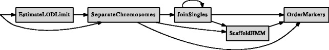
The linkage map construction workflow with LM. The nodes present modules of LM (described in Section 2) and the arrows show the order in which these modules are typically applied

2.1 Notation

Let the input data consist of genotypes of individuals in k families, or crosses, over n SNP markers. Each family has two parents (P generation) and their offspring (F₁ generation). Without loss of generality, we assume that each family consists of exactly m offspring.

We denote the two homozygous genotypes as 0 and 1, heterozygous genotype as 2 and missing genotype as −1. A marker is maternally (paternally) informative in a family if the mother (father) of this family is heterozygous. The haplotypes (alleles inherited together from one parent) of each offspring can be partially deduced from the genotypes of the offspring and its parents (trios). We denote these haplotype alleles as 0 or 1 and missing or unknown haplotype as −1. We define maternal (paternal) segregation pattern for a marker and a family as a string of maternal (paternal) haplotype alleles at that marker.

2.2 Separate chromosomes and join singles: the marker assignment modules

The module SeparateChromosomes assigns markers into LGs as follows:

1. Filtering and haplotype deduction. Probable errors and inconsistencies are filtered out from the data, and partial haplotypes are deduced from genotype trios (see Section 2.2.1).

2. The following steps are repeated until the LG assignment of markers converges:

   1. All marker pairs that have a LOD score are joined together to form LGs.
   2. Completing the haplotypes. Achiasmatic meiosis is used to correct and impute genotypes (see Section 2.2.2).

Several LOD scores can be provided in descending order for each LM run. If the maximum LOD score obtained with some marker is lower than the first limit, the next limit is used instead. This option is useful when there are several families, and the maximum LOD score may differ based on how many families are informative on each marker. Step 2b can be disabled in LM to study species without achiasmatic meiosis.

The module JoinSingles can be used to add single markers, not assigned originally to any LG, to existing LGs. For each single marker, a multipoint LOD score is computed by inspecting several markers (within a given similarity) of the existing LGs to find more informative families. Each single marker is joined only if it can be linked uniquely to a LG.

2.2.1 Filtering and haplotype deduction

LM filters out SNPs for which the offspring allele distribution deviates too much from the expected Mendelian proportions [segregation distortion in Cheema and Dicks (2009)]. Genotype errors are modeled by allowing each underlying haplotype to be incorrect with an independent probability ε specified by the user. Sum of squares is computed between expected and observed allele distributions separately for each family. If the P-value of this sum in a family is lower than a given parameter δ, the SNP is discarded from that family.

During the filtering, any missing parental genotypes are imputed if possible. There is also the option to cope with cases where both parents are missing and only one parent is informative. Filtering is also possible based on the proportion of missing genotypes, parental genotype combination and the number of identical segregation patterns.

Following filtering, the haplotypes of each offspring are deduced from the genotype trios. Because of uninformative trios and missing genotypes, only partial haplotypes can be deduced.

2.2.2 Completing the haplotypes

Assuming achiasmatic meiosis, there are only two maternal haplotypes for each chromosome. This observation is used by clustering maternal haplotypes over each LG into two similar groups with small Hamming distance (Hamming, 1950) within groups. By using the consensuses of both groups as true haplotypes, missing genotypes are imputed and erroneous genotypes are corrected. This provides more complete haplotype information, which allows LM to place more markers more accurately both into and within chromosomes (see Section 3.3).

The decision problem corresponding to the clustering of haplotypes into two similar groups with minimum Hamming distance can be shown to be NP-complete (proof omitted). If the data are error-free, the optimal clustering can be found efficiently in polynomial time (by checking whether a graph is bipartite). As the rate of genotyping errors is usually relatively low (due to filtering), typical instances are easy to solve. The following algorithm is used for haplotype clustering:

1. For each family and LG, the maternally informative markers are processed in ascending order of missing haplotypes. The maternal segregation pattern of each marker is either complemented or not, to obtain a phased pattern. The phase is chosen to make the new pattern as similar as possible to the previously phased patterns.

2. A consensus segregation pattern is constructed for each LG by taking the most common alleles from the phased patterns.

3. This consensus (or its complement) is used as the true maternal segregation pattern for each marker.

2.3 Choosing LOD score limit L

LM can choose LOD score limit(s) L automatically. The module EstimateLODLimit accomplishes this task by generating 100 datasets, by permutating the input genotypes of each offspring, separately for each marker. Maximum LOD score is computed from these datasets, which defines the empirical distribution from which the value of L can be chosen with a desired significance level. LM will display the P-value and the expected number of joined marker pairs and triplets for each positive limit. Several limits can be found by first finding one and then re-estimating new limit(s) among marker pairs that cannot obtain as high LOD score as the previous limit.

2.4 Marker ordering

The module OrderMarkers orders markers within each LG as follows:

1. Steps filtering and haplotype deduction and completing the haplotypes are performed (see Sections 2.2.1 and 2.2.2)

2. Initial order. Initial marker order for paternally informative markers is found in a greedy fashion (see Section 2.4.1)

3. Refining order. Starting from the initial order, marker orders are changed locally to maximize the likelihood of the order, which gives the final marker order (see Section 2.4.2).

2.4.1 Initial order

First, the recombination fractions between all informative marker pairs are computed. To be able to explore possible several locally optimal orders, the search of the initial order is randomized by adding random noise to the recombination fractions to obtain distances between the markers. The distance used is a linear combination of the recombination fraction and a value sampled from a beta () distribution, where a and b are the number of recombinant and non-recombinant haplotypes, respectively (). The amount of noise can be controlled by a user-specified parameter giving the linear combination coefficient between 0 (no noise) and 1 (beta sample). Adjacent marker pairs are then added to the solution in ascending order of distance, making sure that no loops are formed and no more than two neighbors per marker are added. After each marker pair has been added, new distances are computed between the newly constructed chain of two or more adjacent markers and all other markers and chains. This is done in such a manner that if the end point marker of a chain is not informative in some family, the next informative marker toward the other end of the chain is used to compute the respective recombination fraction with added noise. Only a subset of the smallest distances between markers is stored to avoid quadratic memory requirement.

2.4.2 Refining order and the likelihood computation

Given the initial order with N markers, random local changes (illustrated in Fig. 2) to this order are evaluated and accepted if the likelihood is improved. Our experiments showed no significant improvement by using more sophisticated search strategy, such as the simulated annealing (Kirkpatrick et al., 1983), in this step.

Fig. 2.

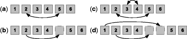
Local changes used in order refinement include (a) swapping two markers in the order, (b) moving one marker to a new place in the order, (c) reversing the order of three or more adjacent markers and (d) moving the prefix or suffix of the order to a new position with or without reversing

For now, let us assume a fixed order of markers for which the likelihood is computed. Furthermore, we assume that the phase of each marker is known, i.e. we know whether the segregation patterns should be complemented or not to obtain partly missing inheritance vectors. The recombination events (and haplotype errors) are detected by differences (Hamming errors) in these vectors. More precisely, while reading the markers in the fixed order, a change in an individual’s value from 1 to 0 or from 0 to 1 indicates recombination. The number of these changes ( or ) is denoted as COUNT, and a solution with a small COUNT is desired.

LM computes the likelihood of marker order by using a standard hidden Markov model (HMM). This model has states 0 and 1 for each marker, and transitions are allowed only between states of adjacent markers. A transition from state 0 to 1 or from 1 to 0 between markers j and is made with probability given by the corresponding recombination fraction r_j. Each state emits either s with probability or with probability e_j, and thus e_j gives the haplotype error probability for marker j. The HMM is learned with the Baum-Welch expectation maximization (EM) algorithm (Durbin et al., 1998) from the partial inheritance vectors. In this manner, the likelihood computation is efficient (linear time), compared with solutions in which the actual inheritance vectors are enumerated [e.g. Lander and Green (1987)].

It is also possible to use fixed values for both or one of r_j and e_j. If both are fixed, there is no need for the EM-algorithm and likelihood computation becomes faster. Moreover, fixing error parameters to some small value would make the likelihood non-invariant to end point symmetries (swapping of the two last or the two first markers) as described in Cartwright et al. (2007). There is also an option to deal with these symmetries by specifying a penalty parameter α to use ‘likelihood - COUNT’ as the optimization score.

LM chooses the phases of the segregation patterns to obtain partial inheritance vectors by minimizing COUNT. If there are no missing haplotypes, the inheritance vectors can be obtained simply by inspecting patterns of adjacent informative markers. However, with an excessive number of missing values, the corresponding decision problem can be shown to be NP-complete (proof omitted).

Typically, however, the mapping minimizing COUNT is easy to find. LM finds suitable mapping by first inspecting only segregation patterns of adjacent informative markers. Next it analyzes whether the mapping can be improved by complementing partial inheritance vectors obtained so far. This mapping corresponds to the two-way pseudo-test cross, discussed in van Os et al. (2005b). LM does the mapping independently for each order to be evaluated, which allows the mapping to vary as the optimal order is being searched for.

2.5 The ScaffoldHMM module

The module ScaffoldHMM uses marker positions on genome scaffolds to assign markers into LGs. This option is helpful with datasets containing so few offspring that only maternally informative markers can be separated into chromosomes (achiasmatic meiosis), whereas paternally informative markers can be separated into LGs that cannot be assigned to chromosomes. The proposed framework is suitable for other tasks as well, e.g. to combine linkage maps constructed from different datasets and to find probable scaffolding, mapping and linkage map errors. The input to ScaffoldHMM consists of two linkage maps (or one map twice) with scaffold mappings, and the module calculates the most probable LG (of the first map) and the log-odds of this assignment for each marker and scaffold.

ScaffoldHMM uses HMMs to model mapped markers in scaffolds. Let K be the number of LGs (chromosomes) in the first (input) map. Every scaffold defines a topology for one HMM, which has K states for each mapped marker in the scaffold. The K states of each marker correspond to the K LGs of the first map. There are two types of emission distributions in the model. First one emits LG name (number) from a state that corresponds to the first map. If there are no errors in the first map, state k should always emit name k in this distribution. The second distribution emits LG name of the second map. If there is one-to-one mapping f between the LGs of the input maps, state k should always emit name f(k) in this distribution. The transition parameters corresponding to scaffold errors are fixed based on empirical distance distribution of detected scaffold errors in the first map.

Maximum likelihood emission parameters are learned simultaneously for all HMMs using Baum-Welch algorithm. Posterior decoding (Durbin et al., 1998) is used to compute the probability of each marker being in certain LG k, i.e. the LG name of this mapped marker is emitted from the state k. This approach takes simultaneously into account all scaffolds and LGs to find the most probable LG (chromosome) assignment.

2.6 Asymptotic running times and memory space

The asymptotic running time of marker assignment and the estimation of LOD score limit significance is . Thus, it scales quadratically on the number of SNPs n, as each marker pair has to be tested, and linearly on the number of individuals km. The marker ordering phase has asymptotic running time of for one LG with N SNPs. Here the local search procedure to find the maximum likelihood solution dominates the running time as there are local changes to be evaluated. Thus, the marker ordering scales cubically on the number of SNPs and linearly on the number of individuals. LM reduces the latter running time by automatically discarding every marker that is equal to or less informative than some other marker not yet discarded. To further reduce the runtime, it is possible to combine markers with near identical inheritance patterns (up to missing values). However, only O(mnk) space is used, and therefore LM can be applied even to large datasets. ScaffoldHMM has time and space complexity, where K is the number of LGs in the first linkage map given as input.

2.7 Implementation details of LM

The input files of LM are required in pre-makeped LINKAGE (Lathrop et al., 1984) format, and only unphased full-sib families with at most four alleles per marker are allowed. Only paternal haplotypes are used in marker ordering due to the assumption of achiasmatic recombination. To study species without achiasmatic recombination, each individual can be coded as two paternally informative individuals to achieve sex-averaged recombination fractions.

Data from other types of crosses can be analyzed as independent full-sibs. The simulated F2 backcross data in Section 3.3 was analyzed in this manner with LM. Loss of information in this case can be reduced by adding artificial individuals giving the phase of data and/or by coding the SNP values with three or four alleles based on the information given by the cross. In some species, such as the common fruit fly (Drosophila melanogaster), only females exhibit recombination, in which case one may use LM by swapping the sexes in the input data. Any type of cross from which one can separate parents and their offspring can be analyzed with LM.

3 RESULTS

3.1 The Glanville fritillary butterfly data

We constructed a linkage map for the Glanville fritillary butterfly (M.cinxia) with data for four different families. The parents of each family originated from populations from Finland (female) and Spain (male).

Altogether 106 individuals of three families and 4989 SNPs were genotyped with Roche NimbleGen (F. Hoffmann-La Roche Ltd, Switzerland) SNP-chip platform by the manufacturer. In these data, 3941 and 2630 SNPs were maternally and paternally informative, respectively, in one or more families.

The fourth family was genotyped with SOLiD3/5500 sequencing platforms (Life Technologies Ltd, UK) to produce a denser SNP dataset. Sequencing was based on SOLiD RAD tag libraries (Miller et al., 2007), constructed with a newly developed in-house protocol. This dataset consists of sequencing data for 12 offspring and their parents. The raw reads have been mapped with BWA (Li and Durbin, 2009) and SAMtools (Li et al., 2009) to the draft reference genome (Lehtonen et al., in preparation) (109 M mapped reads). SNPs and genotypes have been called using LM (see the Supplement). The number of SNPs was 93 767, of which 43 431 and 62 172 were maternally and paternally informative, respectively. All genotype data are provided as raw signals/counts as well as called genotypes with LM, along with the mapping information of the corresponding SNPs to our draft reference genome.

The chromosome assignment for the NimbleGen data was constructed with SeparateChromosomes using LOD score limit L = 4.4 [obtained by EstimateLODLimit, 5% significance, considering only maternal information () and LGs with three or more markers]. Additional markers were added to these LGs with JoinSingles with L = 6 and all informative markers. A map with 32 LGs and 2928 SNPs was obtained, including one LG with markers following Z chromosomal inheritance, i.e. female offspring are homozygotes of one of the father’s alleles. The smallest LG with three markers segregated according to the sex, and hence we concluded that it consists of pseudo-autosomal regions, homologous regions between the Z and W chromosomes. The pseudo-autosomal LG was merged with the other sex LG, giving 31 LGs with sizes between 29 and 165 markers. The actual number of chromosomes of the Glanville fritillary is 31 (2n = 62) (Federley, 1938).

In the NimbleGen data, the order of markers was obtained by first running OrderMarkers on each chromosome without error modeling. Next, markers with distances of over 20 cM were removed from the ends of each chromosome (total number of markers removed was 42) as likely errors. LM was then rerun on the remaining markers both without and with genotype error modeling (α = 0.1), which resulted in linkage maps of 1704 cM and 1466 cM, respectively.

For the RAD tag data, the maternal map was constructed using SeparateChromosomes with L = 3.2, joining markers with identical maternal segregation patterns. By discarding small LGs, 32 LGs remained. Using JoinSingles with L = 2.3, we obtained a map with 19 896 markers. Finally, we merged the two sex LGs. Because of achiasmatic recombination, this map assigns markers only to chromosomes (not within).

Similarly, a paternal map was constructed by grouping paternally informative markers with identical inheritance patterns. This map had 20 822 SNPs and 423 LGs with two or more markers in each LG. The maternal and paternal maps were combined using ScaffoldHMM based on information on marker positions within reference genome scaffolds. By manually inspecting paternal LGs assigned to each chromosome, each chromosome was split into 4–10 ‘bins’ of paternal LGs. The order of these bins was established during the manual process. Based on the number of the bins (228), the genetic length is estimated to be 1642 cM. More information on the manual process is given in the Supplement. The combined map was used in genome assembly validation (Lehtonen et al., in preparation).

The number of common SNPs in the NimbleGen and RAD tag-based maps is 23. Nonetheless, ScaffoldHMM was able to join the two maps. Chromosome by chromosome comparison of these two maps can be found in the Supplement.

3.2 The squinting bush brown butterfly data

The publicly available data on the squinting bush brown butterfly (Bicyclus anynana) (Beldade et al., 2009) was used to test LM. The data consist of 533 SNPs from 12 families, from which 22 offspring and the parents were genotyped per family.

EstimateLODLimit (5% significance) was used to find the limit , which was used in SeparateChromosomes. We thereby obtained a solution with 29 chromosomes, of which 28 matched uniquely the 28 (2n = 56) chromosomes reported in Beldade et al. (2009). This solution assigned 19 markers to these 28 chromosomes that were not assigned to any chromosome in Beldade et al. (2009), whereas the result in Beldade et al. (2009) included only two markers not assigned to any chromosome by LM.

For curiosity, another map was constructed by considering only maternal information (by setting ). When recombination parameter was set to 0.001, 28 chromosomes matching uniquely to those reported in Beldade et al. (2009) were found (LOD score limits , 5% significance). Adding single markers to the initial LGs using also paternal information with an LOD score limit 5.6, we obtained a map with 19 additional markers compared with 5 in Beldade et al. (2009).

Finally, we ordered the markers within chromosomes. The LM solution orders 70% more markers than reported in Beldade et al. (2009), obtained with CRI-MAP (Lander and Green, 1987). By comparing the results for the subset of markers ordered in Beldade et al. (2009), the likelihoods (computed by LM) of the order found by LM were at least 10-fold better on 10 chromosomes compared with the likelihood of the order given in Beldade et al. (2009). The Supplement shows one example of different orders, obtained by LM and reported in Beldade et al. (2009), where the difference is in the position of SNP C2817P666. We have contacted the authors of Beldade et al. (2009), and they confirmed that based on their new (unpublished) data, the LM position for SNP C2817P666 is correct. These results were obtained automatically by LM, without any manual work and using only a few minutes of computing time.

3.3 Simulated data

We simulated F2 backcross data containing 100 SNPs and 100 individuals in the same fashion as in Wu et al. (2008). The distance of adjacent SNPs was on average 1 cM, whereas the rate of genotype errors γ and missing genotypes η varied as in Wu et al. (2008). For each γ and η, we generated 30 datasets and ran LM, MSTmap (Wu et al., 2008) and R/qtl (Broman et al., 2003). AntMap has only a graphical user interface, and thus it needed manual work for each dataset. Therefore, AntMap (Iwata and Ninomiya, 2006) was applied only to 15 dataset for some γ and η. LM was run with recombination and error parameters fixed (LM) and by learning these parameters (LM-full) from the data. We measured the runtime for each software on a typical desktop computer (Intel Core 2 Duo CPU, 3.16 GHz). The accuracy was measured by computing the number of erroneous marker pairs of the obtained results (unnormalized version of Kendall’s τ statistic, a solution with higher accuracy has less erroneous marker pairs). The error rates and the running times are reported in Table 1.

Table 1.

Comparison of the performance of LM, MSTmap (Wu et al., 2008), AntMap (Iwata and Ninomiya, 2006) and R/qtl (Broman et al., 2003)

γ	η	LM		LM-full		MSTmap		AntMap		R/qtl
		E	Time	E	Time	E	Time	E	Time	E	Time
0.00	0.00	0.70	6	0.57	10	1.13	1	0.67	17	210.43	322
0.00	0.01	29.30	16	32.00	36	31.50	1	—	—	1826.43	633
0.00	0.05	65.07	18	67.63	42	68.63	1	—	—	2087.63	1080
0.00	0.10	117.83	18	115.73	42	134.17	1	—	—	1887.23	1415
0.00	0.15	184.33	18	181.17	42	212.07	2	—	—	1618.03	1835
0.01	0.00	8.47	8	7.97	16	15.03	1	—	—	129.5	465
0.05	0.00	34.03	16	42.23	36	58.47	1	—	—	564.13	525
0.10	0.00	38.50	18	48.57	36	59.90	1	—	—	434.20	528
0.15	0.00	37.27	18	51.20	36	63.17	2	—	—	572.30	559
0.01	0.01	31.33	18	33.03	40	34.13	1	55.07	18	713.47	875
0.05	0.05	63.20	18	72.13	42	77.90	1	711.8	18	747.7	1694
0.10	0.10	159.57	18	146.77	42	155.87	1	—	—	1108.73	2083
0.15	0.15	235.67	18	236.37	42	326.77	2	—	—	1285.57	2317
Multifamily
0.75*	0.00	616.70	1055	679.13	6580	12633.5	331	—	—	—	—
10k
0.00	0.00	4.23	410	2.90	2040	44.43	295	—	—	—	—
0.01*	0.01	1.73	409	1.77	641	7.13	73448	—	—	—	—

Note: Each number is averaged over 30 (15 in AntMap) independent runs. Column E reports the average number of erroneous marker pairs among a subset of markers that can be differentiated based on the data. The running time is in seconds; parameters γ and η give the rates of missing values and genotyping errors, respectively. Best results for each row are shown in boldface. (* = identical markers with missing values are combined with the option missingClusteringLimit in LM to reduce runtime.)

Second, we simulated 30 F2 backcross datasets with 200 individuals and 1000 SNPs. The distance of adjacent markers was on average 0.1 cM and the data were error-free. The individuals were organized into groups of size 20, and each group was set to be missing with probability 0.75, independently for each marker (similar to multifamily full-sib data). The results are reported in Table 1 as ‘multifamily’.

Third, we simulated 30 F2 backcross datasets with 200 individuals and 10 000 SNPs over 100 cM without errors and with a moderate rate of errors and missing data (0.01). These results are denoted as ‘10k’ in Table 1. We were able to run only LM and MSTmap on datasets with (R/qtl ran out of memory, AntMap gave an error message). With 100 000 SNPs we were able to run only LM (data not shown, MSTmap ran out of memory).

LM outperformed the other methods in accuracy, and it was the second fastest following MSTmap on small datasets (others but ‘10k’) but fastest with large numbers of SNPs when noise and missing data were introduced. LM was about as fast as AntMap, but the accuracy of AntMap decreased dramatically as soon noise and missing values were included. Note that the result of LM is not the same on each run as its algorithms are randomized. We have noticed that running LM several times and picking the result with the highest likelihood (or lowest COUNT) improves the quality of results. However, for Table 1 LM was run only once.

The difference in accuracy between LM and LM-full is not large; hence in practice it might be a good idea to use fixed error and recombination parameters to achieve a faster runtime for LM. In fact, for small error rates the performance with fixed parameters seems to be even better, probably because of the fact that LM-full becomes attracted more easily to some locally optimal order. Moreover, the choice of the actual fixed recombination (and error) values was not critical, as values 2-fold higher and lower to the simulated ones worked equally well.

The marker spacing for the simulated F2 data was uniform with adjacent markers being either 1, 0.1 or 0.01 cM apart. When the data were simulated, each individual had a constant probability to recombine between adjacent markers. Thus, the actual distance between markers (based on the data) was distributed according to a binomial distribution. Highest variation was in the datasets with 100 individuals, where most datasets contained adjacent markers with distance of at least 4 cM.

We evaluated different methods also on datasets with greater distance variation. This was achieved by grouping 100 individuals randomly into 10 groups of 10 individuals for each marker, and assuming that all individual in a group recombined with probability 0.02, producing datasets with an average length of 200 cM. The results for these data were not significantly different from the ones in Table 1 (data not shown). Assuming fixed recombination and error parameters, LM performs about as well as if these parameters were learned from the data.

Finally, we simulated 30 datasets with achiasmatic meiosis to evaluate how much the linkage map accuracy could be improved by using achiasmatic meiosis (to complete haplotypes) in LM. Each dataset consisted of four full-sib families with 20 individuals in each, 30 simulated chromosomes, each having 100 SNPs and 100 cM paternal length. The rate of missing genotypes and genotype errors were both 0.01 and the minimum allele frequency for the parents was 0.5.

The chromosome assignment was studied by SeperateChromosomes on a single family with LOD score limit 5.6 and considering only maternal haplotypes. A single run of JoinSingles with LOD score limit 5.6 was performed considering all families and both parental haplotypes with and without haplotype completion. With haplotype completion, we could assign on average 2503 markers to chromosomes, compared with 2460 without completion.

Next the marker ordering was studied by running OrderMarkers on the known chromosome assignments. The average numbers of incorrect marker pairs were 312 (6.8% of all pairs) and 485 (10.5%) with and without haplotype completion, respectively. Thus, we could assign 1.7% more markers into chromosomes and order these markers with 35% lower error rate.

3.4 Discussion of results

We have shown with real and simulated data that LM outperforms other methods compared in this study in accuracy and is generally fast. Moreover, LM is versatile and it can be applied to a wide range of different types of datasets. For instance, it would have been difficult and time-consuming to construct linkage maps for the Glanville fritillary data, described in Section 3.1, without LM and its ScaffoldHMM module. For the purposes of genome assembly validation or refinement, relative low map resolution is sufficient (in our case data were obtained from 12 offspring), but the mapped markers must span the entire genome. In particular, most scaffolds should have two or more markers to detect chimeric scaffolds.

The experiments using simulated and real data suggest that LM can use achiasmatic meiosis efficiently to achieve significant improvement in linkage map accuracy.

4 CONCLUSION

We have described a novel tool, Lep-MAP, which can be used to construct accurate linkage maps for large SNP datasets with high rates of noise and missing values, commonly generated by next-generation sequencing. Lep-MAP outperformed other methods compared in this study in accuracy on real and simulated data. It is light-weight in computation burden and highly automated, allowing fast and objective linkage map construction.

REFERENCES

- Baxter S, et al. Linkage mapping and comparative genomics using next-generation RAD sequencing of a non-model organism. PLoS One. 2011;6:e19315. doi: 10.1371/journal.pone.0019315. [DOI] [PMC free article] [PubMed] [Google Scholar]
- Beldade P, et al. A gene-based linkage map for Bicyclus anynana butterflies allows for a comprehensive analysis of synteny with the lepidopteran reference genome. PLoS Genet. 2009;5:e1000366. doi: 10.1371/journal.pgen.1000366. [DOI] [PMC free article] [PubMed] [Google Scholar]
- Broman K, et al. R/qtl: QTL mapping in experimental crosses. Bioinformatics. 2003;19:889–890. doi: 10.1093/bioinformatics/btg112. [DOI] [PubMed] [Google Scholar]
- Cartwright D, et al. Genetic mapping in the presence of genotyping errors. Genetics. 2007;176:2521–2527. doi: 10.1534/genetics.106.063982. [DOI] [PMC free article] [PubMed] [Google Scholar]
- Cheema J, Dicks J. Computational approaches and software tools for genetic linkage map estimation in plants. Brief. Bioinform. 2009;10:595–608. doi: 10.1093/bib/bbp045. [DOI] [PubMed] [Google Scholar]
- de Givry S, et al. Carthagene: multipopulation integrated genetic and radiation hybrid mapping. Bioinformatics. 2005;21:1703–1704. doi: 10.1093/bioinformatics/bti222. [DOI] [PubMed] [Google Scholar]
- Doerge R. Mapping and analysis of quantitative trait loci in experimental populations. Nat. Rev. Genet. 2002;3:43–52. doi: 10.1038/nrg703. [DOI] [PubMed] [Google Scholar]
- Durbin R, et al. Biological Sequence Analysis: Probabilistic Models of Proteins and Nucleic Acids. Cambridge: Cambridge University Press; 1998. [Google Scholar]
- Ehrlich P, Hanski I. On the Wings of Checkerspots: A Model System for Population Biology. New York: Oxford University Press; 2004. [Google Scholar]
- Federley H. Chromosomenzahlen finnländischer Lepidopteren. I. Rhopalocera. Hereditas. 1938;XXIV:397–464. [Google Scholar]
- Garey M, Johnson D. Computers and Intractability: A Guide to the Theory of NP-Completeness. NY, USA: W.H. Freeman & Co.; 1979. [Google Scholar]
- Hamming R. Error detecting and error correcting codes. Bell Syst. Tech. J. 1950;29:147–160. [Google Scholar]
- Iwata H, Ninomiya S. Antmap: constructing genetic linkage maps using an ant colony optimization algorithm. Breed. Sci. 2006;56:371–377. [Google Scholar]
- Jansen J, et al. Constructing dense genetic linkage maps. Theor. Appl. Genet. 2001;102:1113–1122. [Google Scholar]
- Kirkpatrick S, et al. Optimization by simulated annealing. Science. 1983;220:671–680. doi: 10.1126/science.220.4598.671. [DOI] [PubMed] [Google Scholar]
- Laird N, Lange C. Genetic Dissection of Complex Traits, volume 60 of Advances in Genetics. Academic Press; 2008. Family-based methods for linkage and association analysis; pp. 219–252. [DOI] [PubMed] [Google Scholar]
- Lander E, Green P. Construction of multilocus genetic linkage maps in humans. Proc. Natl Acad. Sci. USA. 1987;84:2363–2367. doi: 10.1073/pnas.84.8.2363. [DOI] [PMC free article] [PubMed] [Google Scholar]
- Lathrop G, et al. Strategies for multilocus linkage analysis in humans. Proc. Natl Acad. Sci. USA. 1984;81:3443–3446. doi: 10.1073/pnas.81.11.3443. [DOI] [PMC free article] [PubMed] [Google Scholar]
- Li H, Durbin R. Fast and accurate short read alignment with Burrows-Wheeler transform. Bioinformatics. 2009;25:1754–1760. doi: 10.1093/bioinformatics/btp324. [DOI] [PMC free article] [PubMed] [Google Scholar]
- Li H, et al. The sequence alignment/map format and SAMtools. Bioinformatics. 2009;25:2078–2079. doi: 10.1093/bioinformatics/btp352. [DOI] [PMC free article] [PubMed] [Google Scholar]
- Lincoln S, Lander E. Systematic detection of errors in genetic linkage data. Genomics. 1992;14:604–610. doi: 10.1016/s0888-7543(05)80158-2. [DOI] [PubMed] [Google Scholar]
- Miller M, et al. Rapid and cost-effective polymorphism identification and genotyping using restriction site associated DNA (RAD) markers. Genome Res. 2007;17:240–248. doi: 10.1101/gr.5681207. [DOI] [PMC free article] [PubMed] [Google Scholar]
- Morton N. Sequential tests for the detection of linkage. Am. J. Hum. Gen. 1955;7:277–318. [PMC free article] [PubMed] [Google Scholar]
- Stam P. Construction of integrated genetic linkage maps by means of a new computer package: join map. Plant J. 1993;3:739–744. [Google Scholar]
- Van Ooijen J. Multipoint maximum likelihood mapping in a full-sib family of an outbreeding species. Genet. Res. 2011;93:343–349. doi: 10.1017/S0016672311000279. [DOI] [PubMed] [Google Scholar]
- van Os H, et al. Record: a novel method for ordering loci on a genetic linkage map. Theor. Appl. Genet. 2005a;112:30–40. doi: 10.1007/s00122-005-0097-x. [DOI] [PubMed] [Google Scholar]
- van Os H, et al. Smooth: a statistical method for successful removal of genotyping errors from high-density genetic linkage data. Theor. Appl. Genet. 2005b;112:187–194. doi: 10.1007/s00122-005-0124-y. [DOI] [PubMed] [Google Scholar]
- Wu Y, et al. Efficient and accurate construction of genetic linkage maps from the minimum spanning tree of a graph. PLoS Genet. 2008;4:e1000212. doi: 10.1371/journal.pgen.1000212. [DOI] [PMC free article] [PubMed] [Google Scholar]
- Yamamoto K, et al. Construction of a single nucleotide polymorphism linkage map for the silkworm, Bombyx mori, based on bacterial artificial chromosome end sequences. Genetics. 2006;173:151–161. doi: 10.1534/genetics.105.053801. [DOI] [PMC free article] [PubMed] [Google Scholar]
- Yasukochi Y. A dense genetic map of the silkworm, Bombyx mori, covering all chromosomes based on 1018 molecular markers. Genetics. 1998;150:1513–1525. doi: 10.1093/genetics/150.4.1513. [DOI] [PMC free article] [PubMed] [Google Scholar]
Associated Data
This section collects any data citations, data availability statements, or supplementary materials included in this article.