Describing Assay Precision – Reciprocal of Variance is correct, not CV percent: its use should significantly improve laboratory performance

Abstract

Background

Describing assay error as percent coefficient of variation (CV%) fails as measurements approach zero [1]. Results are censored if below some arbitrarily chosen lower limit of quantification (LLOQ). CV% gives incorrect weighting to data obtained by therapeutic drug monitoring (TDM), with incorrect parameter values in the resulting pharmacokinetic models, and incorrect dosage regimens for patient care.

Methods

CV% was compared with the reciprocal of the variance (1/var) of each assay measurement. This method [2] has not been considered by the laboratory community. A simple description of assay standard deviation (SD) as a polynomial function of the assay measurement over its working range was developed, the reciprocal of the assay variance determined, and its results compared with CV%.

Results

CV% does not provide correct weighting of measured serum concentrations as required for optimal TDM. It does not permit optimally individualized models of the behavior of a drug in a patient, resulting in incorrect dosage regimens.

The assay error polynomial described here, using 1/var, provides correct weighting of such data, all the way down to and including zero. There is no need to censor low results, and no need to set any arbitrary lower limit of quantification (LLOQ).

Conclusion

Reciprocal of variance is the correct measure of assay precision, and should replace CV%. The information is easily stored as an assay error polynomial. The laboratory can serve the medical community better. There is no longer any need for LLOQ, a significant improvement. Regulatory agencies should implement this more informed policy.

INTRODUCTION – The Problem with CV%

The percent error of an assay has long been used as the customary measure of assay precision. One measures replicate samples, calculates the mean and SD of those replicates, and expresses this SD as a percent of the measurement itself. This is how CV% has been found.

Laboratories, the FDA, and the College of American Pathologists (CAP), have censored laboratory results when they are below the LLOQ. This, and the regulatory policies based on this erroneous idea, have limited the ability of the laboratory to serve the medical community optimally.

METHODS

Calculating the assay CV%

One obtains replicate samples and measures the concentration of drug present in each. One calculates the mean and standard deviation for each sample, divides each sample SD by the mean sample value, and expresses the result as the percent of the mean (the percent coefficient of variation – CV%) at each measurement. If CV% is greater than 15 or 20%, that result is usually censored because it is believed to be unacceptably imprecise.

Since CV% increases as the measurement approaches zero, when it exceeds the acceptable CV%, the assay is said to have reached the lower limit of quantification (LLOQ). The result is then deliberately withheld (censored), and is reported only as being “less than” the LLOQ. The CAP, to evaluate laboratory quality worldwide, sends out samples of known concentration, receives their results back, and publishes them as measures of quality control, including the SD of the overall sample results.

The relationship between CV%, SD, and the assay measurement can be described as

$$\mathrm{CV}\%=(\text{Assay SD}∕\text{mean assay measurement})\times 100$$ (1)

The key to this relationship is the assay SD, which is obtained by rearranging the above expression as shown in eq (2) below.

$$\text{Assay SD}={\mathrm{A}}_1\mathrm{C}$$ (2)

Where A₁ is a number representing the fraction of the assay measurement represented by the CV%, and C is the mean measured concentration. For example, if the CV were 10%, the value of A₁ would be 0.1. In that case, SD = 0.1C

However, Figure 1, and equations 1 and 2, are not realistic, because the CV% increases as the measured concentration approaches zero. The laboratory community has erroneously believed that when CV% increases as the measurement becomes low, that precision is being lost. Because of this erroneous belief, intuitive rather than scientific judgments have been made about what constitutes an “acceptable” CV%. Measurements below these values, with higher CV%, are regarded as being below the lower limit of quantification (LLOQ) of the assay. The upper acceptable limit of CV% is often arbitrarily taken to be 15 or 20 percent. Measurements below the LLOQ currently are censored, and are reported as being below the LLOQ of the assay.

Figure 1.

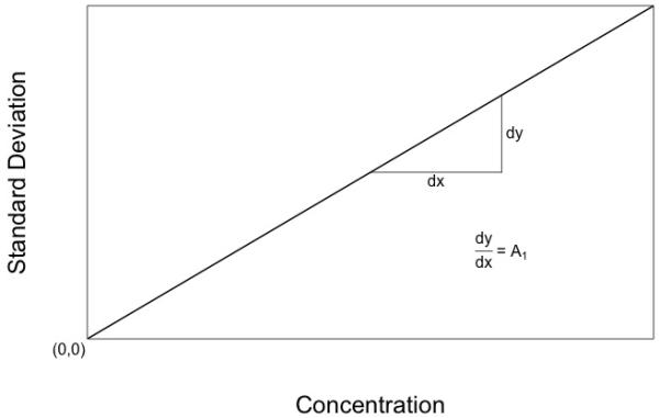
Diagram of an ideal assay with a constant CV%. The assay SD gets smaller and smaller as the measurement approaches zero, and ideally is zero when the measurement is zero.

Jusko [3] discussed the significance of data below the LLOQ. He stated “low concentrations are meaningful and should not be neglected”, and “Repeated measurements below the LLOQ can be assigned a lesser weight based on the actual or expected larger CV% of the analytical method”. However, he did not offer any specific way to determine these weights.

The problem is that as the measurement approaches zero, one enters the region of the assay noise present when the true measurement is zero. This is not accounted for with the above concept of constant CV% as shown in Figure 1 or equations 1 and 2.

However, it is easy to take this into account. One can simply describe the assay SD when a blank sample is measured in replicate, and can call this A₀. Now we have the expression,

$$\text{Assay SD}={\mathrm{A}}_0+{\mathrm{A}}_1\mathrm{C}$$ (3)

where A₀ is the SD of the blank sample, A₁ is defined as above in eqn 2, and C is the mean measured concentration.

This simple addition of a second term describing the SD of a blank sample has a most profound result. One now can accurately describe the assay SD all the way down to and including the blank. There is no longer any need to censor low values. There is, in fact, no LLOQ anymore at all. By introducing C₀, one can describe the SD of an assay all the way down to and including zero. We can see that the entire illusory concept of LLOQ has in fact existed solely because of the incorrect custom of describing assay error as CV%.

The assay CV% is usually not constant over the entire range of the assay. It may change with higher measurements. In this case, one can easily add other terms to this relationship. For example, one can use the expression for a third degree polynomial:

$$\text{Assay SD}={\mathrm{A}}_0+{\mathrm{A}}_1\mathrm{C}+{\mathrm{A}}_2{\mathrm{C}}^2+{\mathrm{A}}_3{\mathrm{C}}^3$$ (4)

where A₀, A₁, A₂ and A₃ are coefficients to be estimated, and C, C², and C³ are the concentration, the concentration squared, and the concentration cubed, respectively. Instead of calculating CV%, we are now calculating the assay SD itself, in the same units as the assay.

If one makes the reasonable assumption that assay noise is normally distributed, the correct way to describe the width of such a Gaussian bell shaped curve is by the reciprocal of the variance of that measurement [2]. The key here is the assay SD. Find the assay SD, square it to get the variance (var). The reciprocal of the variance (1/var) is the correct way to describe assay precision [2].

Calculating the reciprocal of the variance

First, one must measure enough replicate samples to get a reasonable estimate of each sample standard deviation. To do this, we suggest at least five replicates per sample (not just 2 or 3), just as do the FDA Guidelines for Industry [4]. More are always better. The relationship between the number of replicates and the error in the estimate of the sample SD [5,6] is described in eqn (5) and shown in Figure 3.

$$ERRof\sigma \approx \frac{1}{\sqrt{2(n-1)}}$$ (5)

Or, after rearranging, as

$$\frac{ERR}{\sigma }\approx \frac{1}{\sqrt{2(n-1)}}$$ (6)

Where ERR is the standard error of the estimate of the SD (a number from 0 to 1.0), σ is the true value of the SD, n is the number of replicate samples, and ≈ means “approximately equal to”. The more replicates measured, the more precise is the estimate of the SD [5,6]. For 3 samples, ERR is 0.5 or 50%. For n=5, it is 0.353 or 35.3%. For n=9, it is 0.25 or 25%. It seems prudent to use at least five samples for a reasonable estimate of the SD of each sample.

Figure 3.

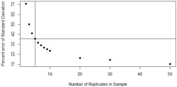
Plot of the standard error of the estimate of the true sample SD versus number of sample replicates [4,5]. Probably at least 5 replicates should be measured, the more the better. Nine replicates, for example, have only half the error of three replicates. The vertical line shows that for 5 replicates, the ERR is 35.3%.

There must be a zero-concentration blank sample to determine the SD of the blank, the machine noise of the assay. Additionally, there should be at least a low sample, a medium one, a high one, and a very high one, to cover the entire working range of the assay.

The relation between the mean assay concentrations and assay SD can be fitted with a polynomial equation as shown in eqn (4). Many software packages do this, including the makeErrorPoly routine in the USC Pmetrics package for population pharmacokinetic (PK) modeling [7]. This polynomial equation can then be stored in the USC Bestdose clinical software [8], (or any similar software) to calculate the SD for each assay sample, square it to get the variance, and calculate 1/var to provide correct weighting of the assay data for the pharmacokinetic (PK) analysis of that drug. In this way, the optimal PK model, either for an individual patient or for populations of patients receiving a drug, can be made from drug assay data, permitting optimal individualized drug dosage for each patient [7-10]. Use of such a polynomial provides an easy and practical way to describe and store the correct error pattern of any assay.

RESULTS – APPLICATION TO REAL ASSAY DATA

Examining an Assay for Vancomycin

Figure 4 illustrates this process for vancomycin. The data shown are taken from CAP samples sent to participating clinical laboratories [11]. It shows the results of fifteen vancomycin quality control samples which were measured by the chemiluminescence assay and reported by 198 to 202 laboratories (not all laboratories reported on all 15 samples). Sample concentrations ranged from 5.61 to 33.383 ug/ml. Figure 4 shows the relationship between the assay measurements and the SD’s of the reported results.

Figure 4.

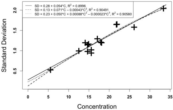
Relationship between measured serum vancomycin concentrations in CAP quality control samples [10] and the assay SD’s. Horizontal axis – measured vancomycin concentrations (ug/ml). Vertical axis – Standard deviation (ug/ml).

A Caveat

Just as with CV%, it is dangerous to extrapolate any polynomial equation beyond the range of its raw data. For example, there is significant doubt from the above vancomycin data about what the assay SD is at the blank, and especially at concentrations over 33 ug/ml.

The SD of the vancomycin blank here may be between about 0.1 and 0.3 ug/ml. This is why one needs specifically to determine the SD at the blank.

Peak vancomycin concentrations are often greater than 33 ug/ml. If we use the first degree polynomial, a concentration of 60 ug/ml has an estimated SD of 3.547 ug/ml. If we use the second, it is 2.8828 ug/ml. If we use the third, it is only 1.4618 ug/ml. This is due to the downward curvature shown in Figure 4 as the concentrations increase, because of the negative coefficients in the second and third degree polynomials. All SD estimates above 33 ug/ml are therefore questionable based on this data.

For example, if we estimate the SD for an assumed measurement of 100 ug/ml, a not uncommon peak value, the first degree polynomial estimates the SD at 5.723 ug/ml. However, that found with the second degree is only 3.001 ug/ml. and the third degree polynomial results in a total impossibility, as the estimated SD has become negative, minus 8.787 ug/ml! That simply cannot be. All values of SD must be greater than zero. We now see the dangers. Polynomial estimates, just like CV%, cannot be trusted outside the ranges of their raw data.

Another example – Voriconazole

At Children’s Hospital of Los Angeles, therapeutic drug monitoring (TDM) of voriconazole employs an Absciex LCMS-MS assay [12,13], a nonparametric population pharmacokinetic model of voriconazole [14], and the USC Bestdose clinical software [7,8]. The assay It is a quantitative MRM analytical method by ESI-LC/MS/MS (ABSiex 400 Q-Trap) which was developed utilizing Positive mode to quantitate Voriconazole (m/z 350.1/281.20) using D3-Voriconazole (m/z 353.1/284.2) as an internal standard. The assay is linear from 0.0 to 30 μg/ml.

The error pattern of this assay was analyzed using 7 samples, each measured in quintuplicate. The samples were a blank, 0.02 ug/ml, 0.5 ug/ml, 5.0, 12.5, 30, and 40 ug/ml. These seven samples gave mean values ± standard deviations (SD’s) of 0.00592 ± 0.000239, 0.177 ± 0.00118, 0.487 ± 0.0121, 5.364 ± 0.8385, 13,94 ± 0.1342, 29.58 ± 0.642, and 38.54 ± 0.381 ug/ml respectively.

When that data was analyzed with the makeErrorPoly function in Pmetrics [7] the following relationships were found, as shown in Figure 5.

Figure 5.

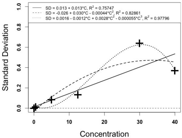
Plot of Voriconazole measured concentrations (horizontal), and assay standard deviation (vertical). The solid line represents the graph of the first degree polynomial, the dashed line the second degree polynomial, and the dotted line the third degree polynomial.

In this figure, the third degree polynomial fits the data best, as expected, but has a marked downward curve at the high end, dangerous if extrapolated any higher. The second degree polynomial has a less pronounced downward curve, and may perhaps be useful, as not many measurements are to be expected to be over 40 ug/ml. However, it may well overestimate the assay SD in the more frequent range from 10 to 25 ug/ml. Because of this, and because the data point at 30 ug/ml is the only one departing from the otherwise general tendency for a straight line relationship, we chose to employ the first degree polynomial, in this particular case, as providing a reasonable and safe description of the error pattern of this assay. Again, other assays [15] have higher order polynomials that fit their particular error data well, which in their cases provide better information for those assays than the first order polynomials shown in the present report.

An example of Gentamicin

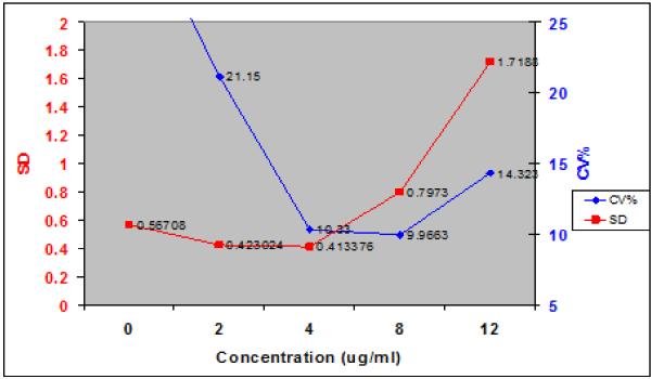
In the Emit gentamicin assay from the Los Angeles County Medical Center, more was done to capture the information over what was then taken to be close to the full working range of the assay. Both SD and CV% are shown in Figure 6. The polynomial relationship between the assay and its SD was:

$$\mathrm{SD}(\mathrm{ug}∕\mathrm{ml})=0.56708-0.10563\mathrm{C}+0.016801{\mathrm{C}}^2$$ (8)

Figure 6.

Relationship between measured gentamicin concentrations and SD, and CV%. Solid squares and Left hand vertical scale – assay SD. Solid circles and Right hand vertical scale – CV%. Note that the relationship between concentrations and CV% is at least as nonlinear as is that between measurement and SD. Note also that the 2 and 4 ug/ml measurements have almost the same SD’s, and yet the CV% of the lower one is about 20% (unacceptable?) while that of the higher measurement is only about 10% (acceptable?). This is a good example of how CV% breaks down as the measurements get smaller.

In this figure, the 2.0 and 4.0 ug/ml measurements have almost the same SD, and therefore, both measurements are almost equally precise. However, the higher measurement has a CV of only 10.3%, while the lower one has a CV% essentially twice as large. This illustrates well the danger of using CV% as a measure of assay precision.

DISCUSSION

It is prudent to examine data covering the entire range of the assay. The assay SD’s must always be positive and realistic. If that is done, one can feel safe using the polynomial fitting the data best. Sometimes the full third degree polynomial is good, especially if its plot is concave upward at the high end. Sometime one may settle for a second degree polynomial if it also is straight or concave upward. Examples of this can be seen from CAP data from an earlier report [15]. Further, in that earlier data, the CAP had covered much more of the working ranges of several assays. They often tended to show a gentle upward concavity which again shows the utility of this method of describing assay errors [15].

The above CAP data for vancomycin provide an estimate of assay precision only over the range of their chosen samples, where measurements are made most often. There is no evidence here to suggest any systematic effort by the CAP to examine assay precision over its full working range.

Within-day and between-day variability

It has been common to report within day and between day variability. However, it is impossible to use this information any further. It is probably most useful to incorporate all data into an overall general assay error polynomial, to develop an error model of the many random events to which a single drug sample is subjected as it goes through a laboratory’s assay system.

Assay error analysis can be repeated whenever desired. New data can be evaluated with respect to the previous error polynomial. If the relationship between sample means and SD has changed, the assay has drifted. One may develop a new polynomial, or re-evaluate the assay itself. On the other hand, if it is similar, it can be included with the previous data, developing a still richer and more informative understanding of the assay.

Those who individualize drug dosage regimens for patients need to fit serum concentration data having the correct quantitative measure of precision so that the optimal pharmacokinetic model can be made for that patient, yielding the drug dosage regimen to hit a clinically selected target serum concentration goal for each patient most precisely, especially using the method of multiple model (MM) dosage design, for example [9,10].

Some vancomycin monitoring guidelines have stated that peak concentrations have no clinical significance [16]. We strongly feel that this is not correct. Vancomycin has toxicity as well as therapeutic effect. Its bacterial killing is non-concentration-dependent [17], but this probably is not the case at all for toxicity. Peak concentrations, while having some further effect on killing the organism, clearly represent increased exposure of the patient to a toxic drug. Well known general strategies for the design of optimal TDM protocols [18] show that even a minimal drug model always has at least 2 model parameters (volume and either elimination rate constant or clearance) and that a minimum of 2 samples is therefore required to make an optimal 1 compartment individualized clinical pharmacokinetic model of drug behavior. Vancomycin peak concentrations are needed as well as troughs to evaluate possible toxicity and to better estimate area under the concentration curve (AUC) even with minimal precision. Ignoring these general principles leads to less informed strategies for individualized dosage regimens of any drug. In addition, vancomycin has at least 2 compartment behavior, and such a model is required to obtain realistic estimates of its serum concentration profile over time, and the resulting AUC.

Defining the Lower Limit of Assay Detection (LLOD) is improved

Because the SD of the blank is determined, rather than setting the smallest possible movement of the detector, one can set a desired criterion of probability (number of blank SD’s above the blank, often 2, 3, or 5, for example, for 95 or 99% or greater probability) with which one decides to accept a forensic result as indicating that a substance is present in the sample or not.

CONCLUSION

Reciprocal of measurement variance is the correct measure of assay precision

Assay measurements errors consist of additive noise, which is assumed to be independent from one measurement to another, and from the model PK parameter values to be estimated. Because of this, if one fits a PK model to assay data, its most likely parameter estimate will be obtained only if each data point is correctly weighted by the reciprocal of its variance [2]. This is easy to do, with no significant change in cost or effort over determining the usual CV%. This approach was first described in [19], and was expanded in [15]. The present paper now provides full, rigorous, mathematical, statistical and visual support for this improved approach [1,2,5,6].

The Assay Error Polynomial provides a practical way to store the error data

After one has obtained the standard deviations of the assay data from the replicate samples, It is easy and practical to store that error pattern in the form of a polynomial for easy reference is reporting the results of any measurement.

Relationship to other clinical sources of error in the therapeutic environment

To determine the additional contribution of the other errors in the clinical environment in which drug therapy takes place, one can calculate an additional noise term in the population PK model of the drug. Such a model describes past experience with the drug, and provides the Bayesian prior for the process of planning, monitoring, and adjusting drug dosage regimens specifically tailored for each individual patient [9,10]. In the Pmetrics population modeling package [7], the additional noise present in the clinical environment is called lambda. Using both 1/var and lambda, clinical and laboratory uncertainties can be independently determined in Bayesian individualization of drug dosage regimens for optimally precise patient care, with optimal knowledge about and management of both the laboratory and the clinical sources of uncertainty.

One can stop censoring low measurements

Using 1/var rather than CV% also eliminates the erroneous perceived need to censor low values below some arbitrarily assigned LLOQ. Eliminating LLOQ is a most significant benefit, avoiding wasted samples or ad hoc methods to compensate for arbitrarily censored data [20,21].

This approach is not limited to drug assays. HIV and HCV PCR results can also be reported in this more informed manner. Clinicians now can follow these results all the way down to zero, to document whether or not the illness is optimally treated. If a patient with HIV has a value reported as <50 copies, one patient might have a value of 45, another only 3, for example. This important result has been deliberately withheld from those ordering the test, simply because of the erroneous belief in CV%. Instead of reporting a result as “less than 50 units/ml”, for example, one can report it both ways, as “16 units/ml, below the old lower limit of quantification of 50 units/ml” for example. The SD of that result can always be obtained from the laboratory if the clinician wishes, and, better yet, the TDM personnel have what is needed (and optimal!) for correct drug dosage individualization.

The awkward use of CV% can now be replaced by a more informed and correct measure of assay precision. 1/var is based on sound mathematical and statistical methods and should replace CV%. It provides the correct measure of assay precision. Further, 1/var eliminates the need to censor low data. It eliminates the need for having any LLOQ at all. It also improves the ability of any assay to provide more rigorous criteria for forensic detection of the presence of a substance in a sample. FDA regulations dealing with this subject [4], and the quality control policies of the CAP [11], for example, can easily be updated to be in accord with modern statistical and mathematical practice. Dr. Jusko’s intuition [3] was on the right track.

Figure 2.

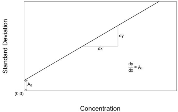
Diagram of an ideal assay with a constant CV%, but with an extra coefficient describing the assay SD (the measurement noise) when the true measurement is actually zero. The assay SD decreases as the measurement approaches zero, but still remains positive and finite as the blank value is encountered.

References

- 1.Spiegel M. Theory and Problems of Statistics. Schaum’s Outline Series. Schaum; New York: 1961. p. 73. [Google Scholar]
- 2.DeGroot M. Probability and Statistics. 2nd ed Addison-Wesley; Reading MA: 1989. pp. 403–423. [Google Scholar]
- 3.Jusko W. Use of pharmacokinetic data below lower limit of quantification values. Pharm Res. 2012;29:2628–31. doi: 10.1007/s11095-012-0805-6. [DOI] [PMC free article] [PubMed] [Google Scholar]
- 4.FDA guidance for industry bioanalytical method validation. http://www.fda.gov/cder/guidance/4252fnl.pdf.
- 5.Ahn S, Fessler JA. Technical report. The University of Michigan; Jul 24, 2003. Standard errors of mean, variance, and standard deviation estimators. [Google Scholar]
- 6.Seber G, Wild C. Nonlinear regression. Wiley; New York: 1989. pp. 536–37. [Google Scholar]
- 7.Neely M. Pmetrics. A software package in R for parametric and nonparametric population modeling and Monte Carlo simulation. Available from www.lapk.org.
- 8.Jelliffe R, Bayard D, Schumitzky A, Milman M, Jiang F, Leonov S, et al. A new clinical software package for multiple model (MM) mesign of drug dosage regimens for planning, monitoring, and adjusting optimally individualized drug therapy for patients; Presented at the 4th International Meeting on Mathematical Modeling, Technical University of Vienna; Vienna, Austria. February 6, 2003. [Google Scholar]
- 9.Jelliffe R, Bayard D, Milman M, Van Guilder M, Schumitzky A. Achieving target goals most precisely using nonparametric compartmental models and “Multiple Model” design of dosage regimens. Ther Drug Monit. 2000;22:346–53. doi: 10.1097/00007691-200006000-00018. [DOI] [PubMed] [Google Scholar]
- 10.Bayard D, Jelliffe R, Schumitzky A, Milman M, Van Guilder M. Selected Topics in Mathematical Physics, Professor R. Vasudevan Memorial Volume. Allied Publishers Ltd.; Madras, India: 1995. Precision drug dosage regimens using multiple model adaptive control: Theory, and application to simulated vancomycin therapy; pp. 407–26. [Google Scholar]
- 11.College of American Pathologists (CAP) Survey C-C. 2011:132. Survey C-A. 2012:128. and Survey C-B. 2012:129.
- 12.Decosterd L, Rochat B, Pesse B, Mercier T, Tissot F, Widmer N, et al. Multiplex ultra-performance liquid chromatography-tandem mass spectrometry method for simultaneous quantification in human plasma of fluconazole, itraconazole, hydroxyitraconazole, posaconazole, voriconazole, voriconazole-N-oxide, anidulafungin, and caspofungin. Antimicrob Agents Chemother. 2010;54(12):5303–15. doi: 10.1128/AAC.00404-10. [DOI] [PMC free article] [PubMed] [Google Scholar]
- 13.Alffenaar J, Wessels A, van Hateran K, Greijjdanus B, Kosterink J, Uges D. Method for therapeutic monitoring of azole antifungal drugs in human serum using LC/MS/MS. J Chromatog B Analyt Technol Biomed Life Sci. 2010;878(1):39–44. doi: 10.1016/j.jchromb.2009.11.017. [DOI] [PubMed] [Google Scholar]
- 14.Neely M, Rushing T, Kovacs A, Jelliffe R, Hoffman J. Voriconazole Pharmacokinetics and Pharmacodynamics in Children. Clinical Inf Dis. 2010;50:27–36. doi: 10.1086/648679. [DOI] [PMC free article] [PubMed] [Google Scholar]
- 15.Jelliffe R, Schumitzky A, Van Guilder M, Liu M, Hu L, Maire P, et al. Individualizing drug dosage regimens: Roles of population pharmacokinetic and dynamic models, bayesian fitting, and adaptive control. Ther Drug Monit. 1993;15:380–93. [PubMed] [Google Scholar]
- 16.Rybak M, Lomaestro B, Rotschafer J, Moellering R, Craig W, Billeter M, et al. Therapeutic monitoring of vancomycin in adult patients: A consensus review of the American Society of Health-System Pharmacists, the Infectious Diseases Society of America, and the Society of Infectious Disease Pharmacists. Am. J. Health-System Pharmacy. 2009;66:82–98. doi: 10.2146/ajhp080434. [DOI] [PubMed] [Google Scholar]
- 17.Larsson A, Walker K, Raddatz J, Rotschafer J. The concentration-independent effect of monoexponential and biexponential decay in vancomycin concentrations on the killing of Staphylococcuss aureus under aerobic and anaerobic conditions. J. Antimicrob Chemotherap. 1996;38:589–97. doi: 10.1093/jac/38.4.589. [DOI] [PubMed] [Google Scholar]
- 18.D’Argenio D. Optimal Sampling Times for Pharmacokinetic Experiments. J. Pharmacokin Biopharmacol. 1981;9:739–56. doi: 10.1007/BF01070904. [DOI] [PubMed] [Google Scholar]
- 19.Jelliffe R. Explicit determination of laboratory assay errors – A useful aid in therapeutic drug monitoring. Drug Monitoring and Toxicology No.DM89-4(DM-56_American Society of Clinical Pathologists Check Sample Continuing Education Program. Drug Monitoring and Toxicology. 1989;10(4) [Google Scholar]
- 20.Bergstrand M, Karlsson M. Handling data below the Limit of quantification in mixed effect models. AAPS J. 2009;11:371–80. doi: 10.1208/s12248-009-9112-5. [DOI] [PMC free article] [PubMed] [Google Scholar]
- 21.Beal S. Ways to fit a PK model with some data below the quantification limit. J Pharmacokinet Pharmacodyn. 2001;28:481–504. doi: 10.1023/a:1012299115260. [DOI] [PubMed] [Google Scholar]