Classification in DTI using Shapes of White Matter Tracts

Abstract

Diffusion Tensor Imaging (DTI) provides unique information about the underlying tissue structure of brain white matter in vivo, including both the geometry of fiber bundles as well as quantitative information about tissue properties as characterized by measures such as tensor orientation, anisotropy, and size. Our objective in this paper is to evaluate the utility of shape representations of white matter tracts extracted from DTI data for classification of clinically different population groups (here autistic vs control). As a first step, our algorithm extracts fiber bundles passing through approximately marked regions of interest on affinely aligned brain volumes. The subsequent analysis is entirely based on the geometric modeling of the extracted tracts. A key advantage of using such an abstraction is that it allows us to capture invariant features of brains allowing for efficient large sample size studies. We demonstrate that with the use of an appropriate representation of the tract shapes, classifiers can be built with reasonable prediction accuracies without making heavy use of the spatial normalization machinery needed when using voxel based features.

I. Introduction

Neuroimaging researchers increasingly rely on diffusion tensor imaging (DTI) for new insights into the tissue microstructure and organization of brain white matter in vivo. DTI can provide information about the axon bundles of the white matter such as preferred orientation, information about local tissue structure using properties of tensors at each voxel. Using these tensors at each voxel fiber bundles are extracted using various techniques like solving stream-line equations [1], clustering [2], montecarlo based methods [3]. Typically fiber bundles are traced from seed points in regions with anatomical interest. Most approaches to group analysis in the clinical DTI literature have relied on voxel based morphometry (VBM) like approaches which require computationally expensive non-linear diffeomorphic registration which can introduce artifcats in connectivity structures.

Recent advances have been made in using tract based morphometry (TBM) in which they abstract away from voxels and work in the space of streamlines [4], [5]. The main challenge with TBM as mentioned in their paper is the requirement of registering tracts across subjects with nonlinear deformation that might change the actual anatomical significances of the tracts. Using shape representations of tracts can alleviate some of the problems in TBM. [6] presented a shape based normalization and provided evidence for tangible improvements in statistical power. Tract shape modeling has also been used to segment out corresponding region specific tracts across subjects without requiring “registration” of seed points used in tractography [7]. All these studies indicate the power of using shape representations of tracts for DTI group analysis. Such geometric modeling of tracts has been argued to be able to account for errors in normalization [8]. Such techniques also offer a moderate level of invariance to quality variations in the low level data (e.g., different scanning parameters) common in multi-center studies. This is indeed attractive as it can open doors to analyze larger datasets (possibly acquired on different scanners) thus increasing the generalizability of statistical conclusions. Partly motivated by these new results, in this paper we seek to make use of the tractography data in the setting of supervised learning in building a two-class predictor where we address the following question:

1) Can the shapes of tracts be used to classify autistic subjects from controls without requiring tract-tract registration?

To study this question we use white matter tracts seeded in the splenium of the corpus callosum. Corpus callosum has been found to be important in connection with autism ([9], [10]) and pathways in this region have a well known anatomy [7]. Using support vector machine (SVM) as a binary classifier and histogram based shape representation of the tracts we are able to obtain reasonable prediction accuracy of upto 75% with cross-validation. A schematic overview of our classification system is shown in Fig. 1. The subjects are first aligned using simple affine transformations. The fiber bundles passing through seeds identified in the splenium (see Fig. 2) are then aligned using the affine parameters. We build histogram representations of these fiber bundles using 3D version of shape context [11]. To avoid over-fitting and improve classification accuracies non-linear principal component analysis (PCA) ([12]) with histogram intersection kernel [13] is used to project the bins into a low-dimensional feature space. These projections are then input to SVM as feature vectors for binary classification.

Fig. 1.

Schematic overview of the shape based classification system. Subjects are registered to a template using affine transformations. These affine transformations are used to align the tracts passing through the splenium. The tracts are represented using 3D shape context. These histogram based feature vectors are projected into a low dimensional space using non-linear PCA and classified using binary SVM.

Fig. 2.

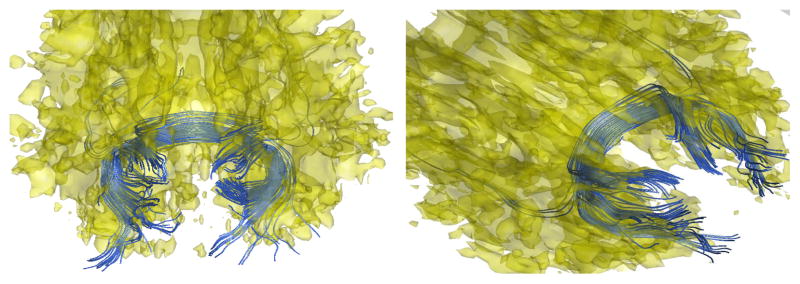
Sample tracts (blue) passing through splenium of the corpus callosum for two subjects.

II. Methodology

A. Data Pre-processing

The DTI data from 73 male subjects were used in this study including 

• 41 subjects with high functioning autism spectrum disorders.

• 32 control subjects matched for age, handedness, IQ, and head size.

Since brain shapes (and hence shapes of tracts) can be affected by factors like age, head size etc., the control subjects were matched for age, handedness, IQ and head size with those of subjects with autism.

Tractography in aligned space tends to suffer from compounding tensor interpolation errors. Hence tracts were extracted in the native space and were then aligned using affine transformations. A second order Runge-Kutta streamline algorithm with TENsor Deflection (TEND) [1] was used to extract the tracts. This gives more robust tracts compared to other streamline algorithms because it uses the entire tensor at each voxel to “deflect” the tracts in contrast to just using the major eigen vector. Fig. 2 shows some sample tracts passing through the splenium for two subjects. The alignment parameters were obtained as follows.

The DTI data from a 16 year old control subject was used as an initial template. The fractional anisotropy (FA) map for this subject was aligned to the MNI-152 white matter prior probability map using an affine transformation and mutual information based cost function with 2mm isotropic resolution over a 91 × 109 × 91 matrix. The FA maps for the other 72 subjects were aligned to this single subject template using a 12-parameter affine transformation with FLIRT (http://www.fmrib.ox.ac.uk/fsl/). The aligned FA maps were then averaged to create an FA template. The FA maps for each subject were again aligned to this template using affine transformation. This secondary normalization step reduced the potential bias issues of using a single subject as a template.

After briefly describing the classification framework in the following section, we explain the feature extraction.

B. Binary Support Vector Classifier

Support vector machines [14] have demonstrated empirical superiority with many theoretical guarantees on their generalization capacity among pattern classification algorithms. Given labeled training data of the form ${\{(y_i,{\mathbf{x}}_i)\}}_{i=1}^N$, with y_i ∈ {−1, +1}, x_i ∈ the algorithm finds a hyperplane w · x − b = 0 by minimizing classification error while maximizing the margin using “boundary examples” or support vectors as:

$$\begin{array}{l}\underset{\mathbf{w},b}{\text{argmin}}\frac{1}{2}{\Vert \mathbf{w}\Vert }^2+C\sum _i{\xi }_i\\ \text{such}\text{that}:y_i(\mathbf{w}·{\mathbf{x}}_i-b)\ge 1-{\xi }_i,\forall i=\{1,2,\dots ,N\}\end{array}$$ (1)

where w is the normal vector, $\frac{b}{\Vert w\Vert }$ is the offset from origin and ξ_i are the slack variables. Using Langrange multipliers the following dual formulation is maximized so that the actually classification can be done by computing dot products with only support vectors:

$$\begin{array}{l}\underset{\alpha }{\text{argmax}}W(\alpha )=\sum _{i=1}^N{\alpha }_i-\frac{1}{2}\sum _{ij}{\alpha }_i{\alpha }_j{y}_i{y}_j{\mathbf{x}}_i^T{\mathbf{x}}_j\\ \text{subject}\text{to}:0\le {\alpha }_i\le C\text{and}\sum {\alpha }_i{y}_i=0\end{array}$$ (2)

where C(> 0) is the tradeoff between regularization and constraint violation. Once we obtain the optimal alpha values (α) the decision function is sign(h(x)), where:

$$h(\mathbf{x})=\sum _{l=1}^m{\alpha }_l{y}_l{\mathbf{x}}^T{\mathbf{x}}_l+b$$ (3)

where ${\{{\mathbf{x}}_l\}}_{l=1}^m$ is the set of support vectors. One of the key design aspects in using SVMs is good feature extraction, i.e. effective representation of x for the data. It is even more crucial with medial data where the number of training examples is usually orders of magnitude low compared to typical machine learning tasks. The goal is to keep the dimensionality of x low while retaining the most useful information to separate the two classes. Hence we use robust histogram based representation of the tract data. To keep the dimensionality low we perform non-linear principal component analysis using histogram intersection kernel [13]. The following two sections describe the histogram representation and non-linear PCA respectively.

C. 3D Shape Context

Typically features used for classification tasks in brain imaging have been raw voxel-level measurements. For each subject all voxels with their values are used as features with some simple preprocessing (like down-sampling [15]) to more complex processing like segmentation using discrimination and robustness measures (DRM) in [16]. Spatial consistency cues are emphasized in a typical feature selection process. They have been used both explicitly and implicity [17]. All of such approaches assume a nearly perfect normalization step since the feature values do not encode any high-level information.

The motivation for our feature extraction is to use the progress made in streamline tractography. By using tracts we are in essense using anisotropic spatial prior in extracting features from DTI data. As mentioned earlier we need good shape representation of tracts that can capture the differences between the two classes. Since we do not expect the subjects to be perfectly aligned, for each subject we build a “context” of the tracts passing through the splenium (see Fig. 2). This is based on the 3D extension of 2D shape context, a very successful descriptor used for shape matching for object recognition [11]. We divide the 3D volume into azimuthal-log-polar bins and count the number of tract control points in each bin. Fig. 3 illustrates the idea in 2D for ease of understanding. Fig. 4(a) shows some sample tracts of a subject with a sample 2D version of binning-frame centered at the splenium. Fig. 4(b) shows the histogram representation for the tracts of that subject. Using medium resolutions (10° bins for azimuthal and polar angles and about 20 bins for logspace radii) helps us cope with slight misalignments since the histograms capture tract control point distributions of tracts which are high-level features as opposed voxel-level features. Such geometric modeling of tracts has been argued to be able to account for errors in normalization [8]. There they use “continuous medial representation (cm-rep)” of the white matter tracts for performing tract based spatial statistics (TBSS) [18]. Histogram based shape modeling offers attractive advantages both in robustness of matching and also computational efficiency [13]. As described in the following section histogram based features allow using histogram intersection kernel to perform efficient non-linear principal component analysis. To our best knowledge, ours is the first effort to study such histogram based modeling of DTI feature extraction in a supervised classification framework.

Fig. 3.

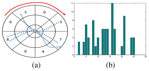
Shape context. Demonstration in 2D for ease of understanding. (a) The log-polar binning used in 2D shape context [11]. Sample 2D streamlines are shown as dotted blue curves. Counts for outermost radial bins are also shown. By reading the bins in the order pointed by the red curve in (a) we obtain the histogram in (b).

Fig. 4.

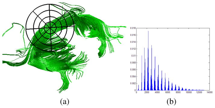
(a) Sample tracts passing through the splenium. A sample 2D version of binning-frame is centered at the splenium. (b) The histogram representation for the tracts.

D. Non-linear PCA using Intersection Kernel

The dimensionality (n) of the features (x) used for a classification influences the complexity of the learnt classifier. The higher the dimensionality the more complex a classifier can be. Even though complex classifiers can provide higher classification accuracies they tend to over-fit the data and lose the generalization ability, indicated by decreased prediction accuracies with cross validation. This is referred to as “curse of dimensionality” which states for a given sample size of training data there is a maximum number of features above which the performance of the classifier decreases. A practical heuristic is to upper bound the dimensionality as $n\le \frac{N}{10}$ where N is the number of training samples. There are several ways to reduce the dimensionality of the feature space. By using 10° bins for azimuthal and polar angles and about 20 bins for logspace radii our histogram representation has 12, 960 bins.

Principal component analysis (PCA) is a dimensionality reduction technique used to select the “basis” features by finding most uncorrelated features. The set of basis features can be obtained by solving for eigen values of the covariance matrix of the data ${\{{\mathbf{x}}_i\}}_{i=1}^N$ [19]. That is one has to solve:

$$\lambda \mathbf{v}=\mathcal{C}\mathbf{v},\text{where}\mathcal{C}=\frac{1}{N}\sum _{i=1}^N{\mathbf{x}}_i{\mathbf{x}}_i^T$$ (4)

where v is the matrix of eigen vectors and λ is the diagonal matrix with eigen values. By selecting the top L largest eigen values the dimensionality can be reduced to L. In some cases where the correlation between features might be high, the above described linear PCA is not powerful enough to reduce the dimensionality. There are several non-linear extensions to perform component analysis like using Hebbian networks, multi-layer perceptrons etc. [20]. But many of those techniques are quite slow. [12] introduced non-linear extension of PCA using “kernel trick” where they replace the dot product in Eq. (4) with a kernel that can simulate dot product in a high-dimensional mapping of the data. The additional technical details of centering the data points before computing the kernel matrix can be found in [12]. We use histogram intersection kernel to compute the kernel matrix. The intersection kernel between two data points is given as:

$$k(\mathbf{x},\mathbf{z})=\sum _{i=1}^{n}min(x(i),z(i))$$ (5)

Using top 6 eigen values we project most histograms onto a 6 dimensional feature space.

III. Experimental Evaluation

Since we have only 73 examples we evaluate our classifier performance using cross-validation scheme. In a k fold cross-validation, the dataset is partitioned into k subsets and each time k−1 samples are used for training and 1 for testing. The process is iterated k times until all the examples are tested once. The prediction accuracies over test subsets are then averaged to report the overall performance of the classifier. The measures reported using cross-validation scheme usually have more statistical significance. We perform leave-one-out cross-validation where k = 73. That is the evaluation is done 73 times each time using 72 examples for training and 1 example for testing until all the examples are tested. The average accuracy over 73 folds is 75.34% with specificity and sensitivity of 71.88%. The classifier output values and the corresponding receiver operating characteristic (ROC) curve are shown in Fig. 5. The average area under curve (AUC) is 0.7645.

Fig. 5.

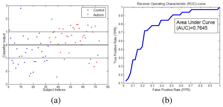
(a) Classifier output (h(x) − b, Eq. (3)) values for the two classes. The thick line is the classification boundary and the dotted lines are the margins. Values above the thick line indicate autism and those below indicate control subjects. Examples inside the margins are harder examples. (b) ROC curve shows that our classifier can perform reasonably well with an area under curve (AUC) of 0.7645. Average specificity and sensitivity is 71.88%. The values are estimated using leave-one-out cross validation.

IV. Discussions and Future Work

Applying machine learning techinques for brain imaging is attracting a significant interest of researchers [21]. Predictors can assist doctors and radiologists to diagonise diseases cost-effectively and efficiently. This paper presents an effort to apply tractography data of DTI to build a binary classifier with resonable prediction accuracy. Tractography data is usually based on anatomical regions of interest. We intend to include tractography data from other anatomically relevant regions for autism like temporal lobe (arcuate fasciculus) to achieve higher accuracies. Autistic patients have problems in understanding language and arcuate fasciculus is thought to be having pathways between regions involved in language understanding. We also intend to work with larger datasets since shape based representations can permit using data from multiple labs more effectively.

References

- 1.Lazar M, Weinstein D, Tsuruda J, Hasan K, et al. White matter tractography using diffusion tensor deflection. Human Brain Mapping. 2003;18(4) doi: 10.1002/hbm.10102. [DOI] [PMC free article] [PubMed] [Google Scholar]
- 2.Savadjiev P, Campbell JS, Pike GB, Siddiqi K. MICCAI. Berlin, Heidelberg: Springer-Verlag; 2008. Streamline flows for white matter fibre pathway segmentation in diffusion MRI; pp. 135–143. [DOI] [PubMed] [Google Scholar]
- 3.King MD, Gadiana DG, Clarka CA. A random effects modelling approach to the crossing-fibre problem in tractography. NeuroImage. 2009 Feb;44(3):753–768. doi: 10.1016/j.neuroimage.2008.09.058. [DOI] [PubMed] [Google Scholar]
- 4.O’Donnel L, Westin CF, Golby A. Tract-based morphometry for white matter group analysis. NeuroImage. 2009;45:832–844. doi: 10.1016/j.neuroimage.2008.12.023. [DOI] [PMC free article] [PubMed] [Google Scholar]
- 5.Goodlett CB, Fletcher TP, Gilmore JH, Gerig G. Group analysis of DTI fiber tract statistics with application to neurodevelopment. NeuroImage. 2009;45(1) doi: 10.1016/j.neuroimage.2008.10.060. [DOI] [PMC free article] [PubMed] [Google Scholar]
- 6.Sun H, Yushkevich P, Zhang H, Cook P, Duda J, Simon T, Gee JC. Shape-based normalization of the corpus callosum for DTI connectivity analysis. TMI. 2007;26 doi: 10.1109/TMI.2007.900322. [DOI] [PubMed] [Google Scholar]
- 7.Bastin M, Piatkowski J, Storkey A, Brown L, MacLullich A, Clayden J. Tract shape modelling provides evidence of topological change in corpus callosum genu during normal ageing. NeuroImage. 2008;43:20–28. doi: 10.1016/j.neuroimage.2008.06.047. [DOI] [PubMed] [Google Scholar]
- 8.Yushkevich P, Zhang H, Simon T, Gee J. MMBIA07. 2007. Structure-specific statistical mapping of white matter tracts using the continuous medial representation. [DOI] [PMC free article] [PubMed] [Google Scholar]
- 9.Lee JE, Hsu D, Alexander A, Lazar M, Bigler E, Lainhart J. ISMRM. 2008. A study of underconnectivity in autism using DTI: W-matrix tractography. [Google Scholar]
- 10.Ke X, Hong S, Tang T, Huang H, Zou B, Li H, Hang Y, Lu Z. An analysis method of the fiber tractography of corpus callosum in autism based on DTI data. IEEE ICBBE. 2008:2409–2413. [Google Scholar]
- 11.Belongie S, Malik J, Puzicha J. Shape matching and object recognition using shape contexts. IEEE Trans Pattern Anal Mach Intell. 2002;24(4):509–522. [Google Scholar]
- 12.Schölkopf B, Smola A, Müller KR. Nonlinear component analysis as a kernel eigenvalue problem. Neural Comput. 1998;10(5):1299–1319. [Google Scholar]
- 13.Maji S, Berg AC, Malik J. Classification using intersection kernel support vector machines is efficient. CVPR. 2008:1–8. [Google Scholar]
- 14.Cortes C, Vapnik V. Support-vector networks. Mach Learn. 1995;20(3) [Google Scholar]
- 15.Vemuri P, Gunter J, Senjem M, Whitwell J, et al. AD diagnosis in individual subjects using struct. MR images. Neu Im. 2008 doi: 10.1016/j.neuroimage.2007.09.073. [DOI] [PMC free article] [PubMed] [Google Scholar]
- 16.Fan Y, Shen D, Gur R, Gur R, Davatzikos C. COMPARE: Classification of morphological patterns using adaptive regional elements. Tran Med Imag. 2007 doi: 10.1109/TMI.2006.886812. [DOI] [PubMed] [Google Scholar]
- 17.Singh V, Mukherjee L, Chung M. Cortical surface thickness as a classifier: Boosting for autism classification. MICCAI. 2008:999–1007. doi: 10.1007/978-3-540-85988-8_119. [DOI] [PubMed] [Google Scholar]
- 18.Smith S, Jenkinson M, Johansen-Berg H, Rueckert D, et al. Nonlinear component analysis as a kernel eigenvalue problem. Neu Img. 2006;31:1487–1505. [Google Scholar]
- 19.Jolliffe I. Principal Component Analysis. Springer; 2002. [Google Scholar]
- 20.Diamantaras K, Kung S. Principal component neural networks: theory and applications. New York, NY, USA: John Wiley & Sons, Inc; 1996. [Google Scholar]
- 21.Pereira F, Mitchell T, Botvinick M. Machine learning classifiers and fMRI: A tutorial overview. NeuroImage. 2009 Mar;45:S199–S209. doi: 10.1016/j.neuroimage.2008.11.007. [DOI] [PMC free article] [PubMed] [Google Scholar]
Associated Data
This section collects any data citations, data availability statements, or supplementary materials included in this article.