

Abstract
Purpose
To assess the test-retest reproducibility of cortical mapping of T2* relaxation rates at 7 T MRI. T2* maps have been employed for studying cortical myelo-architecture patterns in vivo and for characterizing conditions associated with changes in iron and/or myelin concentration.
Materials And Methods
T2* maps were calculated from 7 T multi-echo T2*-weighted images acquired during separate scanning sessions on 8 healthy subjects. The reproducibility of surface-based cortical T2* mapping was assessed at different depths of the cortex; from pial surface (0% depth) towards grey/white matter boundary (100% depth), across cortical regions and hemispheres, using coefficients of variation (COV=SD/mean) between each couple (scan-rescan) of average T2* measurements.
Results
Average cortical T2* was significantly different between 25%, 50% and 75% depths (ANOVA, p<0.001). Coefficient of variations were very low within cortical regions, and whole cortex (average COV = 0.83%–1.79%), indicating a high degree of reproducibility in T2* measures.
Conclusion
Surface-based mapping of T2* relaxation rates as a function of cortical depth is reproducible and could prove useful for studying the laminar architecture of the cerebral cortex in vivo, and for investigating physiological and pathological states associated with changes in iron and/or myelin concentration.
Keywords: 7T, T2*, Reproducibility, Cortex, Myelin, Iron
INTRODUCTION
Ultra-high field magnetic resonance imaging (MRI) (≥7 T) offers higher spatial resolution and signal-to-noise ratio (SNR) than lower field MRI, allowing for better in vivo characterization of human neuroanatomy. Higher field strengths also increase the sensitivity to susceptibility variations across different brain structures, a property that enhances T2*-based contrast driven by susceptibility differences of myelin, iron, calcium and venous deoxyhemoglobin [1]. Studies have reported excellent tissue contrast between grey matter (GM) and white matter (WM) regions on 3D echo-planar imaging (EPI) T2*-weighted magnitude images [2] and within GM and WM regions on gradient recalled echo (GRE) T2*-weighted magnitude images [3, 4] and quantitative maps of the apparent transverse relaxation time T2*[5, 6]. Voxel-wise estimation of T2* relaxation (or R2* = 1/T2*), as opposed to T2*-weighted signal, is a quantitative measure independent of the flip angle, coil sensitivity, scaling parameters and other imaging parameters. T2* decay has been found to inversely correlate with both myelin [6, 7] and iron [8, 9] content.
The degree of myelination in the cortex has been shown in histopathological studies to increase with depth from the pia to the gray matter (GM)-white matter (WM) boundary [10]. Depth-dependent variations in cortical pathology have been demonstrated in autism post mortem [11] and in multiple sclerosis both post mortem and in vivo using quantitative MRI [12–15]. In vivo mapping of T2* within the cerebral cortex from 3D images, however, is challenging due to its thin and circumvolved geometry and its variability across individuals. Surface-based methods [16, 17], which provide a 2D parametric reconstruction of the folded cortex from high-resolution anatomical scans, allow quantification of MRI contrast at different depths within the cortical ribbon. We demonstrated that surface-based mapping of T2* relaxation decay across different cortical regions in vivo is sensitive to the cyto- and myelo-architecture of the cerebral cortex in the healthy brain [6].
Variability in T2* mapping, however, could be introduced and could be mistaken as physiological cortical patterns, or markers of cortical disease. More specifically, variability can be introduced throughout 7T acquisition (day-to-day variability, coil loading, shimming, slice positioning, patient motion) and processing pipeline (segmentation, T2* fitting, registration, surface mapping). This variability remains unknown, preventing from assessing the statistical significance of individual scans and studies in comparison with normative values.
Thus, the main purpose of this work was to asses the test-retest reproducibility of T2* mapping of surface-based measurements of T2* relaxation decay at different depths of the cortical width and across various cortical regions in healthy individuals.
MATERIALS AND METHODS
Subjects
Eight right-handed healthy volunteers (mean ± SD age = 38.5 ± 8.7 years, four females) were recruited for this study. The subjects were pre-screened to exclude any significant medical, neurological or psychiatric condition. Our Institutional Review Board approved all study procedures. Subjects were given a complete description of the study and written informed consent was obtained from each of them.
MRI Data Acquisition
Subjects were scanned on a 7 T whole-body scanner (Magnetom, Siemens Healthcare, Erlangen, Germany), using a SC72 head gradient set and a custom-built 32-channel phased array coil [18]. The subjects were rescanned on the same system between 1 and 3 weeks after the first session. A multi-echo 2D FLASH T2*-weighted spoiled gradient-echo (GRE) pulse sequence was obtained with the following parameters: axial orientation, TR = 2210 ms, TE = 6.44 + 3.32n [n = 0, …,11] ms, flip angle=55°, 2 slabs of 40 slices each to cover the supratentorial brain, FOV= 192 × 168 mm2, in-plane resolution = 0.33 × 0.33 mm2, 1 mm slice thickness (25% gap), bandwidth= 335 Hz/pix, acquisition time (TA) for each slab = 10 min. We also acquired during each session a T1-weighted 3D magnetization-prepared rapid acquisition gradient echo (MPRAGE, TR/TI/TE = 2600/1100/3.26 ms, flip angle=9°, FOV=174 × 192 mm2, resolution = 0.60 × 0.60 × 1.5 mm3, bandwidth =200 Hz/pix, scan time = 5.5 min) sequence for co-registration of 7 T GRE data with cortical surfaces as described previously [4, 6].
In addition to the 7 T sessions, all subjects were scanned once on a 3 T scanner (Tim Trio, Siemens Healthcare) using the Siemens 32-channel coil to acquire a structural scan with a 3D magnetization-prepared rapid acquisition with multiple gradient echoes (MEMPR) (TR/TI=2530/1200 ms, TE=[1.7, 3.6, 5.4, 7.3] ms, flip angle=7°, FOV=230×230 mm2, resolution=0.9×0.9×0.9 mm3, bandwidth=651 Hz/pixel, scan time = 6.5 min) for cortical surface reconstruction using Freesurfer (discussed below) and co-registration with 7 T data.
MRI Data Processing
Processing pipeline for surface-based sampling of T2* measures is illustrated in Figure 1.
Figure 1.

Processing pipeline for obtaining depth-dependent T2* maps. Following T2* fitting, 7 T MPRAGE was registered to the 3 T MEMPR data using FSL FLIRT. The average of the first 4 echoes in each of the 7 T FLASH slab (top and bottom) was initially registered to the 7 T MPRAGE using Freesurfer (FS) ‘tkregister’ to obtain a gross alignment. A finer alignment of 7 T FLASH slabs to the reconstructed surfaces was achieved using a boundary-based registration (FS bbregister) technique with 9 degrees of freedom. T2* was sampled along the entire cortex in right and left hemispheres (RH and LH), at three different depths (25%, 50%, 75%) from pial surface (0% depth) towards GM/WM boundary (100% depth). Inflated surfaces shown in this graphic are from LH.
T2* Fitting
Despite careful B0 shimming, some inhomogeneities remained in some lower brain regions including inferior temporal areas, and in regions at the tissue/air interface (close to the sinuses). These inhomogeneities can induce background field gradients within each voxel, resulting in shorter T2* decay and underestimation of T2* [19]. This effect was compensated by correcting T2* signal at each voxel for susceptibility-induced through-slice dephasing as described previously [6]. A Levenberg–Marquardt non-linear regression model was then used to fit the corrected T2* signal versus TE voxel-wise; R2 goodness of fit was also measured, and voxels with poor fits (R2 <0.9) were excluded from further analyses.
Registration To Surfaces
Freesurfer (FS) (http://surfer.nmr.mgh.harvard.edu/) was used to reconstruct cortical surface models from the 3 T MEMPR data in each individual [16]. In each subject, 7 T FLASH data from both sessions were registered onto the corresponding 3 T surfaces using a two-step procedure [6]. The 7 T MPRAGE was registered to the 3 T MEMPR data using FSL FLIRT (http://www.fmrib.ox.ac.uk/fsl/). The average of the first 4 echoes in each of the 7 T FLASH slab (top and bottom), empirically found to provide adequate SNR and GM/WM contrast, was initially registered to the 7 T MPRAGE (FS tkregister) to obtain a gross alignment. A finer alignment of 7 T FLASH slabs to the reconstructed surfaces was achieved using a boundary-based registration (FS bbregister) technique with 9 degrees of freedom. The registered data (2 slabs per session) were concatenated into a whole brain volume using Freesurfer tools and resampled at 0.33×0.33×0.33 mm3 isotropic resolution.
T2* Sampling In The Cortex
T2* was sampled along the entire cortex in right and left hemispheres (RH and LH), at three different depths (25%, 50%, 75%) from pial surface (0% depth) towards GM/WM boundary (100% depth). T2* measures were averaged for individual cortical regions (provided by the Desikan atlas in Freesurfer) at the three depths.
Test-Retest Reproducibility Assessment
The variance of T2* measures due to different sources (subjects, regions, hemispheres, depths and scan-rescan) was assessed by a component of variance model. Intra-subject reproducibility (scan-rescan at two sessions 1–3 weeks apart) of T2* measurements was expressed in the form of coefficients of variations (COV) [20]. The COVs are the ratios between the SD and the mean of each couple (scan-rescan) of measurements. Scan-rescan COVs were calculated for each cortical region (using the Desikan atlas in Freesurfer), each hemisphere, and at 3 different cortical depths (25%, 50% and 75% from the pial surface). We used analysis of variance (ANOVA) to test T2* heterogeneity across cortical regions defined by the Desikan atlas, in left and right hemisphere. Differences in cortical T2* across the three depths (25%, 50% and 75%) in each hemisphere were assessed using ANOVA, and pairwise T2* differences between each couple of depths using a paired t-test.
RESULTS
Multi-echo T2* data were successfully acquired in all subjects on two occasions. Susceptibility artifacts were minimum in most part of the cortex, though evident in the lower part of the brain (tip of the temporal pole), yielding signal dropout after only few echoes. Average cortical thickness, computed using Freesurfer ranged from 1.73 +/− 0.17 mm in the pericalcarine region to 3.15 +/− 0.1 mm in the insular region. Mean thickness information from all cortical regions can be found in Figure 2.
Figure 2.

Mean (+/− STD) cortical thickness in each of the cortical regions in both hemispheres. The range of cortical thickness was found to be between 1.73 +/− 0.17 mm in the pericalcarine region and 3.15 +/− 0.1 mm in the insular region. Also included in this graphic is a schematic of the Desikan atlas superimposed on the left hemisphere of Freesurfer template ‘fsaverage’ showing the 28 cortical regions investigated in this study. Label 29 corresponds to whole-hemisphere cortical thickness measurements.
T2* Across Cortical Regions
T2* maps at 25%, 50% and 75% depth from the pial surface are shown in Figure 3. Comparison of T2* measurements at 50% depth between session 1 and session 2 in various regions of the cortex for all subjects is presented in Figure 4. T2* varied significantly across regions (ANOVA model, test for heterogeneity, p<0.001) and there was no significant difference across hemispheres (p=0.27). Overall, T2* decreased significantly with sampling depth towards WM interface (ANOVA model, p<0.001). Global average T2* at 25%, 50% and 75% depth was 33.77, 32.18 and 30.29 ms, respectively.
Figure 3.
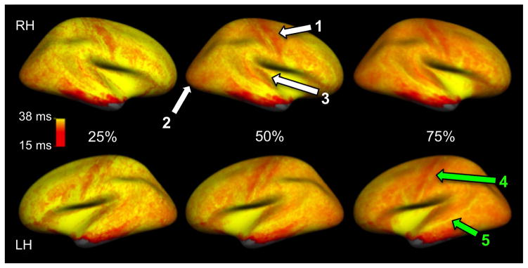
T2* mapping in the right (RH) and left (LH) hemispheres at 25%, 50% and 75% depth from the pial surface (0% being the pial surface, 100% being the white/gray matter interface). T2* measures were averaged across all eight subjects and across both sessions. Shorter T2* was observed in the myelin-rich ‘precentral’, ‘lateral occipital’ and ‘transverse temporal’ regions indicated by white arrows ‘1’, ‘2’ and ‘3’, respectively. Green arrows ‘4’ and ‘5’ point to patterns of longer T2* observed in the central sulcus and the superior temporal sulcus.
Figure 4.
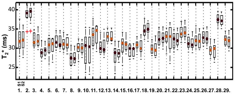
Median T2* with 25th percentile at session 1 (S1) and session 2 (S2) for 28 regions defined by the Desikan atlas (gyrus-based) within the left hemisphere (LH). Label 29 corresponds to whole-hemisphere T2* measurements. The legend for the different labels has been presented in Figure 2. This figure illustrates the low variability between scan-rescan T2* measurements.
Patterns of shorter T2* were found in the ‘precentral’, ‘lateral occipital’ and ‘transverse temporal’ regions, which correspond to the sensorimotor, visual and auditory cortices (indicated in Figure 3 by arrows ‘1’, ‘2’ and ‘3’ respectively). The superior frontal and the cingulate regions show longer T2*. A bright band of longer T2* along the central sulcus is clearly visible at the three depths (arrow ‘4’ in Figure 3), relative to the adjacent myelin-rich precentral and post central gyri. A similar band of longer T2* is visible along the superior temporal sulcus (arrow ‘5’ in Figure 3), pronounced at at 50% and 75% depths. T2* measurements at each cortical depth for both hemispheres averaged across all subjects and sessions, and p values of pairwise differences in T2* between each couple of depths are reported in Table 1.
Table 1.
T2* values averaged across sessions and across cortical regions for each hemisphere at each depth. SD=standard deviation (across 8 subjects). T2* varied significantly between the three depths (ANOVA, p<0.001), but not between hemispheres (p=0.27). Paired t-test for T2* differences between each couple of depths were also significant. T2* decay is shorter in the deeper layers of the cortex, close to the white matter and longer close to the pial surface.
| Hemisphere | Depth from pial surface | Mean T2* (ms) | SD | p-value (paired t-test) |
|---|---|---|---|---|
| Right | 25% | 33.84 | 1.46 | # p=0.001 |
| ## p=10−5 | ||||
| 50% | 32.19 | 1.35 | ### p=0.02 | |
| 75% | 30.31 | 1.52 | - | |
| Left | 25% | 33.69 | 1.53 | # p=0.003 |
| ## p=10−5 | ||||
| 50% | 32.17 | 1.53 | ### p=0.03 | |
| 75% | 30.27 | 1.57 | - |
p= T2* at 25% versus T2* at 50%;
p= T2* at 25% versus T2* at 75%;
p= T2* at 50% versus T2* at 75%.
Test-Retest Reproducibility
T2* measurements from session 1 and session 2 showed excellent reproducibility across cortical regions as compared to between subjects variability, as illustrated in Figure 4. The COVs of T2* values across individual cortical regions ranged from 0.5% to 6.5% (average COV across all regions, across depths = 1.66%). COVs between sessions for the whole cortex at 25%, 50% and 75% depths were 0.83%, 1.79% and 0.87%, respectively. The mean COVs in each cortical region are reported in Figure 5.
Figure 5.
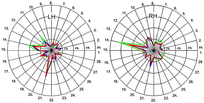
Coefficients of variation (in %) of T2* for 28 cortical regions defined by the Desikan atlas. Color code: Green, red and blue colors in the plot represent 25%, 50% and 75% depths from the pial surface, respectively. This figure illustrates the high inter-session reproducibility of T2* quantification. Mean COV’s for average T2* at 25%, 50% and 75% depths were 0.77%, 1.96% and 1.01% for LH and 1.04%, 1.78% and 1.06% for RH. The legend for the different labels can be found in Figure 2.
DISCUSSION
Our results showed that T2* measurements from surface-based analysis are highly reproducible and as such could be potentially used to assess changes in myelin and / or iron concentration in the cortex in the clinical setting. The high reproducibility is likely due to an optimized acquisition and processing strategy detailed by Cohen-Adad [21].
Cortical T2* contrast has been associated predominantly with non-heme iron stored in ferritin particles [22]. T2* contrast also reflects myelin content as non-heme iron is co-localized with myelin on cellular and molecular levels in healthy cortical laminae [23]. Water trapped in myelin has shorter T2 relaxation time (~20 ms at 3 T) than water within intra/extracellular compartments (~80 ms at 3 T), which may also contribute to shorter T2* in the presence of myelin [7, 24]. This dependence has enabled the use T2*-weighted imaging to investigate the laminar structure of healthy cerebellar cortex [25] and to study pathological changes within the cortex in demyelinating disorders such as multiple sclerosis [26].
We found a ‘strip’ like pattern of longer T2* in the superior temporal sulcus when compared to the adjacent myelin-rich gyri. In addition, longer T2* was found in the superior and middle frontal sulci, and the cingulate regions, consistent with previous observations [6]. Similar concordance was also observed with appearance of longer T2* along the posterior bank of the central sulcus.
Shorter T2* was found in the sensorimotor, visual and auditory cortices, in line with previous T2* studies [6, 27]. Similar spatial patterns were observed using quantitative T1 [28–30] and T1-/T2-weighted imaging [31] and are likely driven by higher myelin density in these regions.
Imperfect registration across T1-T2* modalities does exist in spite of the boundary-based approach that may lead to deviations in the sampling depths at a few vertices (total vertices ~ 160,000). However, we observed a very high scan-rescan reproducibility of our depth-specific T2* measurements from MRI data acquired at different sessions. This suggests that imperfect registration might occur in a very small fraction of the vertices, and may not have an adverse effect on T2* mapping at various cortical depths. In order to maintain the total scan time within reasonable time limits for in vivo studies as well as in the clinical setting, we acquired anisotropic data with very high in-plane resolution (0.33 × 0.33 mm2), and 1 mm slice thickness. This voxel shape likely introduced a bias in the quantification of T2* across the cortical ribbon, given that the partial volume effect was not the same for different orientation of the cortical surface with respect to the orientation of the slice. Moreover, as demonstrated in [6], cortical T2* is influenced by the orientation of cortical fibers relative to B0 rendering estimation of intrinsic T2* difficult. However, the only aim of this study was to assess test-retest reproducibility, not bias. Future work should aim at correcting for the above limitations with the help of accelerated high-resolution isotropic acquisitions and accurate modeling of B0 orientation-dependence.
In conclusion, we report a high reproducibility of in vivo surface-based measurements of T2* relaxation rate at 7 T in the healthy human cerebral cortex. Surface-based analysis of T2* as a function of cortical depth is a reproducible tool for studying the cerebral cortex in vivo. Surface-based T2* mapping can also be used to understand and potentially quantify the pathophysiology and progression of diseases associated with changes in cortical iron and/or myelin concentration.
Acknowledgments
Grant support:
This work was supported by a grant of the National Multiple Sclerosis Society (NMSS [4281-RG-A-1 to C.M.], the Claflin Award, and partly by the National Center for Research Resources [P41-RR14075, and the NCRR BIRN Morphometric, Project BIRN002, U24 RR021382].
Dr Cohen-Adad was supported by a fellowship from the NMSS [FG 1892A1], FRQS and NSERC.
Dr Louapre has received lecture fees from Novartis and research support from ARSEP foundation.
References
- 1.Chavhan GB, et al. Principles, techniques, and applications of T2*-based MR imaging and its special applications. Radiographics. 2009;29(5):1433–49. doi: 10.1148/rg.295095034. [DOI] [PMC free article] [PubMed] [Google Scholar]
- 2.Zwanenburg JJ, et al. Fast high resolution whole brain T2* weighted imaging using echo planar imaging at 7T. Neuroimage. 2011;56(4):1902–7. doi: 10.1016/j.neuroimage.2011.03.046. [DOI] [PubMed] [Google Scholar]
- 3.Li TQ, et al. Extensive heterogeneity in white matter intensity in high-resolution T2*-weighted MRI of the human brain at 7.0 T. Neuroimage. 2006;32(3):1032–40. doi: 10.1016/j.neuroimage.2006.05.053. [DOI] [PubMed] [Google Scholar]
- 4.Cohen-Adad J, et al. In vivo evidence of disseminated subpial T2* signal changes in multiple sclerosis at 7T: A surface-based analysis. Neuroimage. 2011;57(1):55–62. doi: 10.1016/j.neuroimage.2011.04.009. [DOI] [PMC free article] [PubMed] [Google Scholar]
- 5.Budde J, et al. Human imaging at 9.4 T using T(2) *-, phase-, and susceptibility-weighted contrast. Magn Reson Med. 2011;65(2):544–50. doi: 10.1002/mrm.22632. [DOI] [PubMed] [Google Scholar]
- 6.Cohen-Adad J, et al. T(2)* mapping and B(0) orientation-dependence at 7 T reveal cyto- and myeloarchitecture organization of the human cortex. Neuroimage. 2012;60(2):1006–14. doi: 10.1016/j.neuroimage.2012.01.053. [DOI] [PMC free article] [PubMed] [Google Scholar]
- 7.Hwang D, Kim DH, Du YP. In vivo multi-slice mapping of myelin water content using T2* decay. Neuroimage. 2010;52(1):198–204. doi: 10.1016/j.neuroimage.2010.04.023. [DOI] [PubMed] [Google Scholar]
- 8.Langkammer C, et al. Quantitative MR imaging of brain iron: a postmortem validation study. Radiology. 2010;257(2):455–62. doi: 10.1148/radiol.10100495. [DOI] [PubMed] [Google Scholar]
- 9.Peran P, et al. Volume and iron content in basal ganglia and thalamus. Hum Brain Mapp. 2009;30(8):2667–75. doi: 10.1002/hbm.20698. [DOI] [PMC free article] [PubMed] [Google Scholar]
- 10.Braitenberg V. A note on myeloarchitectonics. The Journal of comparative neurology. 1962;118:141–56. doi: 10.1002/cne.901180202. [DOI] [PubMed] [Google Scholar]
- 11.Stoner R, et al. Patches of Disorganization in the Neocortex of Children with Autism. New England Journal of Medicine. 2014;370(13):1209–1219. doi: 10.1056/NEJMoa1307491. [DOI] [PMC free article] [PubMed] [Google Scholar]
- 12.Mainero C, et al. A gradient in intracortical laminar pathology in multiple sclerosis: an in vivo study at 7 Tesla MRI. Multiple Sclerosis Journal. 2013;19(11):429–429. [Google Scholar]
- 13.Louapre C, et al. Intracortical laminar pathology in the motor cortex is associated with proximal underlying white matter injury in multiple sclerosis: a multimodal 7 T and 3 T MRI study. Multiple Sclerosis Journal. 2013;19(11):8–8. [Google Scholar]
- 14.Derakhshan M, et al. Surface-based analysis reveals regions of reduced cortical magnetization transfer ratio in patients with multiple sclerosis: a proposed method for imaging subpial demyelination. Hum Brain Mapp. 2014;35(7):3402–13. doi: 10.1002/hbm.22410. [DOI] [PMC free article] [PubMed] [Google Scholar]
- 15.Tardif CL, et al. Quantitative magnetic resonance imaging of cortical multiple sclerosis pathology. Mult Scler Int. 2012;2012:742018. doi: 10.1155/2012/742018. [DOI] [PMC free article] [PubMed] [Google Scholar]
- 16.Dale AM, Fischl B, Sereno MI. Cortical surface-based analysis. I. Segmentation and surface reconstruction. Neuroimage. 1999;9(2):179–94. doi: 10.1006/nimg.1998.0395. [DOI] [PubMed] [Google Scholar]
- 17.Waehnert MD, et al. Anatomically motivated modeling of cortical laminae. Neuroimage. 2014;93(Pt 2):210–20. doi: 10.1016/j.neuroimage.2013.03.078. [DOI] [PubMed] [Google Scholar]
- 18.Keil B, et al. Design Optimization of a 32-Channel Head Coil at 7T. Proceedings of the 18th Annual Meeting of ISMRM; 2010; Stockolm, Sweden. [Google Scholar]
- 19.Fernandez-Seara MA, Wehrli FW. Postprocessing technique to correct for background gradients in image-based R*(2) measurements. Magnetic resonance in medicine: official journal of the Society of Magnetic Resonance in Medicine / Society of Magnetic Resonance in Medicine. 2000;44(3):358–66. doi: 10.1002/1522-2594(200009)44:3<358::aid-mrm3>3.0.co;2-i. [DOI] [PubMed] [Google Scholar]
- 20.Abdi H. Coefficient of Variation. In: Salkind N, editor. Encyclopedia of Research Design. SAGE Publications, Inc; Thousand Oaks, CA: 2010. pp. 170–172. [Google Scholar]
- 21.Cohen-Adad J. What can we learn from T2* maps of the cortex? Neuroimage. 2014;93(Pt 2):189–200. doi: 10.1016/j.neuroimage.2013.01.023. [DOI] [PubMed] [Google Scholar]
- 22.Fukunaga M, et al. Layer-specific variation of iron content in cerebral cortex as a source of MRI contrast. Proc Natl Acad Sci U S A. 2010;107(8):3834–9. doi: 10.1073/pnas.0911177107. [DOI] [PMC free article] [PubMed] [Google Scholar]
- 23.Connor JR, et al. Cellular distribution of transferrin, ferritin, and iron in normal and aged human brains. J Neurosci Res. 1990;27(4):595–611. doi: 10.1002/jnr.490270421. [DOI] [PubMed] [Google Scholar]
- 24.Sati P, et al. Micro-compartment specific T2() relaxation in the brain. Neuroimage. 2013;77:268–78. doi: 10.1016/j.neuroimage.2013.03.005. [DOI] [PMC free article] [PubMed] [Google Scholar]
- 25.Marques JP, et al. Cerebellar cortical layers: in vivo visualization with structural high-field-strength MR imaging. Radiology. 2010;254(3):942–8. doi: 10.1148/radiol.09091136. [DOI] [PubMed] [Google Scholar]
- 26.Mainero C, et al. In vivo imaging of cortical pathology in multiple sclerosis using ultra-high field MRI. Neurology. 2009;73(12):941–8. doi: 10.1212/WNL.0b013e3181b64bf7. [DOI] [PMC free article] [PubMed] [Google Scholar]
- 27.Deistung A, et al. Toward in vivo histology: a comparison of quantitative susceptibility mapping (QSM) with magnitude-, phase-, and R2*-imaging at ultra-high magnetic field strength. Neuroimage. 2013;65:299–314. doi: 10.1016/j.neuroimage.2012.09.055. [DOI] [PubMed] [Google Scholar]
- 28.Weiss M, et al. Quantitative T1 mapping at 7 Tesla identifies primary functional areas in the living human brain. 19th Annual Meeting of ISMRM; 2011. [Google Scholar]
- 29.Geyer S, et al. Microstructural Parcellation of the Human Cerebral Cortex - From Brodmann’s Post-Mortem Map to in vivo Mapping with High-Field Magnetic Resonance Imaging. Frontiers in human neuroscience. 2011;5:19. doi: 10.3389/fnhum.2011.00019. [DOI] [PMC free article] [PubMed] [Google Scholar]
- 30.Sereno MI, et al. Mapping the Human Cortical Surface by Combining Quantitative T1 with Retinotopy. Cerebral cortex. 2012 doi: 10.1093/cercor/bhs213. [DOI] [PMC free article] [PubMed] [Google Scholar]
- 31.Glasser MF, Van Essen DC. Mapping human cortical areas in vivo based on myelin content as revealed by T1- and T2-weighted MRI. The Journal of neuroscience: the official journal of the Society for Neuroscience. 2011;31(32):11597–616. doi: 10.1523/JNEUROSCI.2180-11.2011. [DOI] [PMC free article] [PubMed] [Google Scholar]