Neurons in the Most Superficial Lamina of the Mouse Superior Colliculus Are Highly Selective for Stimulus Direction

Abstract

The superior colliculus (SC) is a layered midbrain structure important for multimodal integration and sensorimotor transformation. Its superficial layers are purely visual and receive depth-specific projections from distinct subtypes of retinal ganglion cells. Here we use two-photon calcium imaging to characterize the response properties of neurons in the most superficial lamina of the mouse SC, an undersampled population with electrophysiology. We find that these neurons have compact receptive fields with primarily overlapping ON and OFF subregions and are highly direction selective. The high selectivity is observed in both excitatory and inhibitory neurons. These neurons do not cluster according to their direction preference and lack orientation selectivity. In addition, we perform single-unit recordings and show that direction selectivity declines with depth in the SC. Together, our experiments reveal for the first time a highly specialized lamina in the most superficial SC for movement direction, a finding that has important implications for understanding signal transformation in the early visual system.

Introduction

The superior colliculus (SC) in mammals [or optic tectum (OT) in lower vertebrates] is a midbrain structure involved in multimodal sensorimotor integration, saccade generation, and orientating head and body movements (May, 2006; Gandhi and Katnani, 2011). The superficial layers of the SC, including the stratum griseum superficiale (SGS) and stratum opticum, are purely visual and receive direct retinotopic inputs from the retina. The intermediate and deep layers of the SC are multimodal and premotor, containing auditory, somatosensory, and eye movement maps that are aligned with the retinotopic maps in the SGS. Such a layered organization facilitates the integration of visual, auditory, and tactile information and the initiation of orienting movements to redirect attention toward a stimulus (Cang and Feldheim, 2013).

Studies in a number of species, including goldfish, zebrafish, mice, rats, and tree shrews, indicate that visual layers in the SC/OT can be further divided into sublaminae (Albano et al., 1978; Schmidt, 1979; Girman and Lund, 2007; Huberman et al., 2008; Gabriel et al., 2012). For example, in mice, a subtype of ON–OFF direction-selective (DS) retinal ganglion cells (the DRD4 RGCs) was found to project exclusively into the upper SGS (Huberman et al., 2009). In contrast, the transient OFF α-RGCs project into the lower SGS (Huberman et al., 2008). Thus, these studies suggest that the visual layers of the SC may receive a stack of superimposed retinotopic inputs that each encodes a different feature of the visual world (Dhande and Huberman, 2014). However, the functional properties of SGS neurons cannot be inferred easily from anatomical projection patterns, in part because different RGC subtypes often project to the same SGS sublaminae. For example, the upper SGS, in addition to receiving DS input from DRD4 and other types of RGCs (Kay et al., 2011), is also the primary, if not exclusive, target of the W3 RGCs, which are motion sensitive but not DS (Kim et al., 2010; Zhang et al., 2012). In addition, the information carried by RGC axons is likely further transformed by local circuits in the SC through dynamic interactions between excitatory and inhibitory inputs, thereby endowing individual SGS neurons with particular functional properties.

Several electrophysiology studies have described the receptive field (RF) properties of visual collicular neurons in mice (Dräger and Hubel, 1975; Wang et al., 2010; Gale and Murphy, 2014). However, despite thorough characterizations in these investigations, no studies have examined the response properties of SGS neurons by sublaminae or depth. In fact, the topmost lamina of the SGS is often undersampled, if not entirely missed, by conventional electrophysiology. This is because the electrode tip is usually tens of micrometers below this level before it finally breaks through the collicular membrane and is able to pick up single units. As a result, the RF properties of the neurons in the most superficial lamina of SGS (Fig. 1) remain essentially a mystery. To address this issue, we have performed two-photon calcium imaging in this study to characterize the response properties of neurons in the most superficial lamina of the mouse SGS.

Figure 1.

The most superficial lamina of the mouse SC is densely packed with cells. A, A series of Nissl staining images of a sagittal section of the SC in an adult mouse. Two of these images are shown at higher magnification. This section was ∼500 μm from the midline. In the inset is a schematic of the mouse brain along the rostral (R)–caudal (C) axis, with the red box marking approximately the region shown in the images. B, Images of a coronal section of the SC from a different mouse. This section was ∼1500 μm from the caudal end of the SC, as diagrammed by the red line in the inset. The cortex (Ctx) was removed in both sections. D, Dorsal; V, ventral; L, lateral; M, medial. Scale bars, 100 μm.

Materials and Methods

Animal preparation.

Adult C57BL/6 mice of both genders were used in this study (postnatal days 53–123), including 16 wild-type (WT) and seven transgenic mice that express the red fluorescent protein tdTomato in GAD2-positive (GAD2⁺; GABAergic) neurons. These transgenic mice were generated by crossing homozygous Gad2-IRES–Cre knock-in mice (stock #010802; The Jackson Laboratory; Taniguchi et al., 2011) with homozygous Ai9 Cre reporter mice that have a loxP-flanked STOP cassette preventing transcription of tdTomato (stock #007909; The Jackson Laboratory; Madisen et al., 2010). Both lines of mice were on a C57BL/6 background. The mice were housed under a 12 h light/dark cycle and provided with food and water ad libitum. All animals were used in accordance with protocols approved by Northwestern University Institutional Animal Care and Use Committee.

In both imaging and physiology experiments, the mice were first anesthetized with urethane (1.3 g/kg in sterile saline solution, i.p.) and then sedated with chlorprothixene (10 mg/kg in water, i.m.). Subcutaneous atropine (0.3 mg/kg) and dexamethasone (2 mg/kg) were also administered before the surgery to avoid respiratory secretions and brain edema, respectively. The animals' core temperature was maintained at 37 °C via a rectal probe and a feedback heater (FHC). A thin layer of silicone oil was applied to the eyes to prevent drying.

After the mice were anesthetized, the scalp was shaved and cleaned with betadine and isopropanol. The skin was then removed to expose the skull. After the connective tissue was removed and the area washed with ACSF, a craniotomy was performed on the left hemisphere, starting at the lambda point and extending ∼5 mm both laterally and rostrally. An 18 gauge needle with a beveled tip was linked to a suction line and used to remove the overlying cortical tissue above the SC.

Dye preparation, loading, and imaging.

For every experiment, a fresh solution of the fluorogenic calcium-sensitive dye Cal-520 AM (AAT Bioquest) was prepared. A solution of 20% Pluronic F-127 in DMSO was freshly prepared and sonicated for 10 min. Four microliters of this solution were used to reconstitute 50 μg of powdered Cal-520. The resulting solution was sonicated for another 12–15 min and then brought to a total volume of 40 μl by adding 35.2 μl of a calcium-free solution (in mm: 150 NaCl, 2.5 KCl, and 10 HEPES, pH 7.4) and 0.8 μl of 5 mm sulforhodamine 101 (SR101), to reach a final concentration of 1.13 mm Cal-520 and 100 μm SR101. After 5 more min of sonication, the solution was ready to be bolus loaded. To load the dye solution into the SC, we used a Nanoject II (Drummond) fitted with a glass pipette with a beveled tip at 45° and with an inner diameter of 10–20 μm.

Once the SC was exposed, the pipette containing the dye was lowered into the tissue using a fine hydraulic manipulator. Twenty pulses of 2.3 nl each (46 nl total volume), at 30 s intervals, were delivered to inject the Cal-520 solution at a depth of 500 μm below the surface. The same procedure was repeated after retracting the pipette to a depth of 250 μm. The pipette was left in the tissue for 1–2 min before being slowly retracted. The SC was then covered by ACSF. Imaging was performed 1–2 h after loading.

Once the injection procedure was complete, a small metal plate was mounted on the mouse's head with MetaBond (Parkell), which, when clamped under the microscope, resulted in the imaged SC surface being mostly flat and perpendicular to the objective. A light-shielding cloth was then placed around the craniotomy to block light from the visual stimulus during imaging. The SC was covered by 2.5% agarose in ACSF for stability. Imaging was performed with a two-photon microscope (2P-SGS; Prairie Technologies) at an excitation wavelength of 800 nm and with a 40×/0.8 numerical aperture objective (Leica). Data were acquired using PrairieView software with a spiral scan at 2× optical zoom, resulting in a circular field of view with a diameter of 135 μm. Image resolution was 256 × 256 pixels and the acquisition rate 8.079 Hz. We also took red-channel images of each field of view at excitation wavelength of 800 nm for SR101 (to identify glial cells) and 720 nm for tdTomato (to identify GAD2⁺ cells).

Visual stimuli.

Visual stimuli were generated with MATLAB Psychophysics toolbox (Brainard, 1997; Niell and Stryker, 2008) on a 37.5 × 30 cm LCD monitor (60 Hz refresh rate, ∼50 cd/m² luminance). The monitor was placed 25 cm away from the eye contralateral to the imaging site (the right eye). The screen was also tilted at an angle matching that of the mouse's head, given that the mouse's nose was slightly elevated to correct for the curvature of SC and allow imaging from a relatively flat surface.

To map the RFs of imaged cells, a 5° × 5° white (to map ON) or black (to map OFF) square was flashed on a gray background, in a 6 × 6 grid in a pseudorandom order. The flash duration was 1 s and repeated (at a different location) after a wait period of 3 s to allow for the calcium signal to decay substantially between flashes. The RFs of the imaged areas, which were always rostral to the lambda suture, were approximately between contralateral 20° and 120° horizontally from the vertical meridian and 40° and −45° vertically (with 0° corresponding to the eye level, with negative values for lower visual space, and the majority of RFs fell between 10° and −45°). To determine direction/orientation selectivity, drifting sinusoidal gratings of 12 directions (0–330°, with 30° increments) were presented in a pseudorandom order either within a circular window (30° in diameter and surrounded by a gray background) near the center of the RFs of the imaged cells or full screen of the stimulus monitor. For imaging, the gratings were displayed for 3 s, and a gray background was shown for 5 s between presentations. The spatial and temporal frequencies of the drifting gratings were 0.08 cycles/° and 2 Hz, respectively, chosen according to our previous electrophysiology study of SC neurons (Wang et al., 2010). In addition, we also used full-screen gratings of the same parameters and moving bright bars (5° in width and 30°/s speed) in some of the experiments. For all types of stimuli, five to seven trials of all conditions were presented to the animal. For single-unit recording, the small gratings were presented at four spatial frequencies (0.02, 0.04, 0.08, and 0.16 cycles/°), for a duration of 1.5 s, followed by 0.5 s of gray screen.

Analysis of imaging data.

Custom MATLAB scripts were used to analyze the two-photon imaging data. After the end of recording sessions, all collected frames of individual time series were averaged, and regions of interest (ROIs) were selected on the average images in which cell bodies were clearly identifiable. A few recordings with drifts and large tissue motion in which cell bodies were blurred in the average images were excluded from additional analyses. The ROIs were either polygons or rectangles drawn manually inside cell bodies to measure the intracellular Ca²⁺ signal with minimal neuropil activity contamination. The intensity values for all pixels in each ROI were averaged for each frame to obtain the raw temporal Ca²⁺ signal of the respective cell. From the raw signal, for each stimulus presentation, the relative change in the fluorescence signal from the baseline, i.e., ΔF/F₀ = (F − F₀)/F₀, was calculated as follows. F₀ was the mean of the baseline signal over a fixed interval before stimulus onset. The fixed interval was the last 25% of the duration between stimuli offset and next onset, which was chosen to allow the fluorescence signal from the previous stimulus presentation to decay sufficiently to baseline. F was the fluorescence signal from 250 ms after stimulus onset to 500 ms (for gratings and 100 ms for spots) after stimulus offset (Scott et al., 2013) and was chosen to improve the signal-to-noise ratio.

A cell was considered responsive to flashing spots or drifting gratings if its mean fluorescence during the visual stimulus period (as defined by F above) was >2 SDs above the mean baseline fluorescence (F₀) for at least one of the stimulus conditions (of the 36 positions for spots or 12 directions for gratings). For bars, because the fluorescent signal of the cell rose only when the stimulus entered its RFs, it was considered responsive if the peak of the averaged F over all trials was >3 SDs above F₀ for at least one of the 12 directions. The mean value of ΔF/F₀ for each of the stimulus conditions of flashes and gratings, or peak value for bars, was then used to determine the RF or direction tuning curves for every responsive cell.

The RF area was determined by two methods. First, the ON- and OFF-evoked ΔF/F₀ on the grid were each fitted with a 2D Gaussian distribution with independent SDs, a and b, in the coordinate system defined by the axes of the response field, as shown in the following equation: G(x, y) = $\frac{A}{2\pi ab}\exp \left(\frac{x{\prime }^2}{2a^2}+\frac{y{\prime }^2}{2b^2}\right)$, where x′ and y′ are the polar transformations of space coordinates x and y at an angle θ, along which the Gaussian distribution is oriented (Wang et al., 2010). The area enclosed by the fitted ellipse (with a and b as its semi-major and semi-minor axes) was used to quantify the area covered by each subregion (Area_on and Area_off). Second, the area of each subfield was calculated by counting the area of squares in the grid in which the cell was responsive as determined by the criterion described above (Liu et al., 2014).

The RF center was also determined using two methods. First, the RF center was the location of the maximum response in the fitted Gaussian. Second, the RF center was determined by the following “center-of-mass” equation: RF Center, [x, y] = $\frac{{\displaystyle \sum R_i{r}_i}}{{\displaystyle \sum R_i}}$, where i represents the places in the grid where the cell was responsive. R and r represent the response magnitude (ΔF/F₀) and position vector at the ith location, respectively. The relative spatial relationship of the ON and OFF subregions were quantified by an area ratio: $\frac{{\text{Area}}_{\text{on}}-{\text{Area}}_{\text{off}}}{{\text{Area}}_{\text{on}}+{\text{Area}}_{\text{off}}}$, where the areas were determined in the two ways described above. The values of the area ratio range between −1 and 1, with positive values indicating a larger ON subregion and negative values indicating a larger OFF subregion. To determine the degree of overlap between ON and OFF subregions, an overlap index (OI) was determined using the following equation: OI = $\frac{S_{\text{ON}-\text{OFF}}}{S_{\text{ON}}+S_{\text{OFF}}-S_{\text{ON}-\text{OFF}}}$, where S_ON and S_OFF are the number of squares of the 6 × 6 grid where the cell responded to ON and OFF stimuli, respectively, and S_ON−OFF is the number of squares where the cell responded to both ON and OFF stimuli. The values of OI range between 0 and 1, with larger values indicating a larger degree of overlap.

For direction selectivity, a direction selectivity index (DSI) was calculated as follows: DSI = $\frac{R_{\text{pref}}-R_{\text{opp}}}{R_{\text{pref}}+R_{\text{opp}}}$, where R_pref is the mean ΔF/F₀ value of the cell at the preferred direction (i.e., maximal response), and R_opp is the response of the cell to the direction opposite to the preferred one. In addition, we also calculated a global DSI (gDSI) as the vector sum of responses normalized by the scalar sum of responses (Gale and Murphy, 2014): gDSI = $\frac{{\displaystyle \sum R_{\theta }{e}^{i\theta }}}{{\displaystyle \sum R_{\theta }}}$, where R_θ is the response magnitude (ΔF/F₀) at θ direction of gratings. Similarly, an orientation selectivity index (OSI) and global OSI (gOSI) were calculated, OSI = $\frac{R{\prime }_{\text{pref}}-R_{\text{orth}}}{R{\prime }_{\text{pref}}+R_{\text{orth}}}$, where R′_pref was the mean response of R_pref and R_opp, and R_orth was the mean response to the two directions orthogonal to θ_pref, and gOSI = $\frac{{\displaystyle \sum R_{\theta }{e}^{i2\theta }}}{{\displaystyle \sum R_{\theta }}}$.

Tuning widths were calculated as full-width at half-height (fwhh) by fitting the raw tuning curves with Von Mises function (Oesch et al., 2005; Elstrott et al., 2008): R = $\frac{R_{\max }{e}^{k\cos \left(\theta -\mu \right)}}{e^k}$, where R is the response at the θ direction (in radians), μ is the preferred direction determined by angle of sum vector (∑R_θe^iθ), R_max is the maximum response, and k is the concentration parameter accounting for the tuning width. The fwhh was then calculated as follows: fwhh = $2*a\cos \left[\frac{\ln \left(\frac{1}{2}{e}^k+\frac{1}{2}{e}^{-k}\right)}{k}\right]$.

Two-photon imaging-guided cell-attached recording.

In a few imaging experiments, we performed simultaneous two-photon imaging and cell-attached recording. We used glass electrodes (tip opening, ∼1–2 μm; 1B150F-4; WPI). The electrodes were filled with ACSF (in mm: 125 NaCl, 5 KCl, 10 glucose, 10 HEPES, and 2 CaCl₂, pH 7.4) containing 20 μm Alexa Fluor 594 for visualization under the microscope. Once a neuron of interest was located, the electrode was advanced to its vicinity with a positive pressure of 60–100 mbars. The pressure was then reduced to 20–40 mbars, and the pipette was slowly approached to a position a few micrometers on top of the target cell. The pipette was further lowered down until it was in contact with the cell. An increase in resistance was observed on contact, and the pressure was released. A little bit of suction was applied occasionally to get a good seal that varied anywhere from 30 MΩ to 1 GΩ and to observe spiking activity with a detectable amplitude above the background. A MultiClamp 700B amplifier (Molecular Devices) in current-clamp mode and a System 3 workstation (Tucker-Davis Technologies) were used to record extracellular spiking. The spiking data were then compared with the imaging data for the same cell. In particular, we compared the number of spikes in a given cluster (a 1 s period preceded by 1 s of quiescence) and the amplitude of the corresponding ΔF/F₀ and saw a linear relationship between the two (n = 3 neurons from 3 WT mice; Fig. 2A–D).

Figure 2.

Two-photon calcium imaging of the sSGS in mouse SC. A, Schematic of the experimental setup with simultaneous imaging and cell-attached recording. B, An image of sSGS neurons loaded with the calcium indicator Cal-520 and a pipette filled with 20 μm Alexa Fluor 594. C, Two example traces of fluorescent signal and simultaneous spiking activity (below each calcium trace) during flashing spot stimulus. D, Relationship between the amplitude of fluorescent signal changes and the number of visually evoked spikes. Each data point was one cluster of spikes within a 1 s period and the corresponding ΔF/F₀. Points of the same color were from individual repetitions of the flashing spot stimulus that covered all possible positions on a 6 × 6 grid in a pseudorandom sequence, and the line of the same color was the corresponding linear fit. E, RFs determined from the calcium signal (left) and spikes (right) for the neuron shown in B. The brightness of each square represents the evoked ΔF/F₀ (left) or spike rate (right) by flashing spots at that location. F, Two-photon images showing Cal-520-loaded neurons in the green channel (left), tdTomato-labeled GAD2⁺ neurons in red (center), and a merged image of both (right).

Single-unit recording.

Mice were anesthetized as described previously for imaging and mounted on a stereotaxic frame with ear bars. The same surgical procedure was performed as for imaging to expose the SC. Tungsten microelectrodes (5–10 MΩ; FHC) were used for single-unit recordings. The surface was estimated as the point at which the electrode touches the SC surface and forms a closed circuit. This was further confirmed visually under the microscope. Agarose was then added onto the recording site to stabilize the brain and kept moist with ACSF throughout the recording session. The electrode was then lowered slowly, perpendicular to the surface, into the SC, and the depth of every recorded unit was noted. Two to three electrode penetrations were performed per animal, yielding one to five units in total. Spikes and field potentials were acquired using a System 3 workstation (Tucker-Davis Technologies) following our published procedures (Wang et al., 2010; Liu et al., 2014; Sarnaik et al., 2014; Zhao et al., 2014).

For each electrode penetration, the RF center was located based on the response of the local field potential to moving bars. Drifting gratings were then presented at that location within a circular window, 30° in diameter, as described above. The direction selectivity of the recorded single unit was quantified using the same DSI as described for imaging.

Nissl staining.

Mouse brains were dissected after perfusion with 4% paraformaldehyde fixative, cryoprotected in 30% sucrose, and embedded in OCT (Tissue-Tek), following our published procedures (Chen et al., 2015). Serial sections of the brains were cut at 14 μm either coronally or sagittally. Sections were then Nissl stained (0.5%; cresyl violet acetate; C5042; Sigma) and coverslipped with Permount (SP15-500; Thermo Fisher Scientific). Images were captured using the DMRB Widefield Fluorescence System (Leica) and assembled in Adobe Photoshop (Adobe Systems).

Statistics.

Statistical analyses and graph plotting were done in MATLAB (MathWorks), and values were presented as mean ± SEM. Statistical tests were performed as described in Results.

Results

Two-photon calcium imaging of the superficial SGS in mouse SC

The most superficial lamina of the SGS, which we refer to as sSGS, appears to be more densely packed with cells than deeper laminae (Fig. 1). To characterize the functional properties of these neurons, we performed in vivo two-photon calcium imaging in urethane-anesthetized adult mice. The SC was exposed after removing overlaying cortical tissues, and sSGS neurons (within the top 50 μm, and the mean depth of the imaged planes was 31.0 ± 2.2 μm, n = 22 recordings) were then loaded with a recently characterized synthetic Ca²⁺ indicator, Cal-520 (Tada et al., 2014). We first characterized the calcium response of the indicator by performing simultaneous two-photon imaging and cell-attached recordings (Fig. 2A–C). We compared the number of spikes and the corresponding fluorescent signal changes (ΔF/F₀; for details, see Materials and Methods) and observed a linear correlation between the two (Fig. 2D). Consistently, the RFs mapped by cell-attached recording and calcium signals displayed a close match in their size and shape (Fig. 2E; for details of mapping RFs, see below), indicating the reliability of Cal-520 over the physiological range of sSGS neurons and its efficacy in measuring their visual response properties.

Thus, we used the Cal-520 indicator to perform two-photon calcium imaging of sSGS neurons in response to primarily two different visual stimuli, flashing spots and drifting gratings, to determine their RF structures and selectivity for stimulus direction and orientation. These experiments were conducted in both WT C57BL/6 and transgenic mice in which GAD2⁺ neurons were fluorescently labeled with tdTomato (GAD2–cre × floxed tdTomato; Madisen et al., 2010; Taniguchi et al., 2011). Imaging these transgenic mice allowed us to compare the response properties of inhibitory GABAergic neurons (GAD2⁺) and putative excitatory neurons [GAD2 negative (GAD2⁻); Fig. 2F]. In total, we imaged the activity of 913 sSGS neurons (388 GAD2⁺ and 472 GAD2⁻ cells from seven GAD2–tdTomato mice, and 53 cells from a WT mouse). The response properties of these neurons are described below.

RF properties of excitatory and inhibitory sSGS neurons

We displayed small bright and dark squares (5° × 5°, on a 6 × 6 grid) on a gray background in a pseudorandom order to map separately the ON and OFF subregions of the RFs of the sSGS neurons (Fig. 2A). For individual recordings, the stimulus screen was placed in front of the contralateral eye such that the RFs of the majority of neurons in the field of view were covered by the 6 × 6 grid. Of the 741 cells we imaged with the “flashing spot” stimuli, ∼64% (n = 477 of 741) and ∼67% (499 of 741) responded to ON and OFF spot stimuli, respectively, with various response magnitudes at different spot locations (Fig. 3A,B; for details of determining responsive cells, see Materials and Methods). The vast majority of the responsive cells responded to both ON and OFF squares (n = 440 of 536), although some responded only to ON (n = 37) or OFF (n = 59) stimuli.

Figure 3.

RF properties of excitatory and inhibitory sSGS neurons. A, ON (red) and OFF (green) RF subregions of two GAD2⁻ neurons determined by two-photon imaging. The brightness of each square represents the evoked ΔF/F₀ by flashing spots at that location according to the scale on the right of each panel. B, ON and OFF RF subregions of two GAD2⁺ neurons. C, D, Distribution histograms of ON (C) and OFF (D) subregion areas of GAD2⁺ (magenta) and GAD2⁻ (blue) neurons, calculated by 2D Gaussian fitting. E, Distribution of the area ratio index between ON and OFF subregions showing a small bias toward negative values, for both GAD2⁺ and GAD2⁻ neurons. F, Distribution of the OI between ON and OFF subregions is biased toward larger values for both groups of neurons.

We next quantified the RF size of the sSGS neurons using two different methods following our previous physiological studies. First, the RF areas were estimated after fitting them with 2D Gaussians (Wang et al., 2010). The majority of RFs were well fitted (88% cells had R² ≥ 0.7 for ON subregions and 89% for OFF) and displayed compact ON and OFF subregions (ON area, 66.7 ± 3 deg² with a median of 55.3, n = 421; OFF area, 71.7 ± 2.9 deg² with a median of 56.8, n = 443). Second, we simply counted the number of grid positions in which significant visual responses were evoked by the flashing spots (Liu et al., 2014) and determined the subregion areas (ON, 154 ± 5 deg² with a median of 150, n = 477; OFF, 173 ± 6 deg² with a median of 150, n = 499). With both measures, the RFs of the sSGS neurons appeared to be smaller than what was reported previously for the whole population of SGS neurons (Wang et al., 2010; Liu et al., 2014). However, more importantly, with two-photon calcium imaging, we were able to analyze separately the RFs of excitatory and inhibitory neurons (Fig. 3A,B). The distributions of RF areas for GAD2⁺ and GAD2⁻ cells were similar to those for the whole population and to each other (Fig. 3C,D; p > 0.05 in all comparisons by the rank-sum test). This is in contrast to the primary visual cortex (V1) in which layer 2/3 inhibitory neurons have larger RFs than excitatory neurons (Liu et al., 2009).

For cells that responded to both ON and OFF squares, we analyzed the relationships between ON and OFF subregions. We compared the ON and OFF subregions by calculating an area ratio index and found its distribution skewed toward negative values (mean ± SEM, −0.05 ± 0.01; median, −0.05; n = 359). This indicates that OFF subregions of the sSGS neurons were slightly larger than their ON subregions, consistent with our previous physiological studies of the entire SGS population (Wang et al., 2010). In addition, the ON and OFF subregions of these neurons were highly overlapping, with the distribution of the OI skewed toward 1 (mean ± SEM, 0.56 ± 0.01; median, 0.57; n = 440), again similar to what was observed in the previous study (Wang et al., 2010). The OFF subregions were similarly larger than ON subregions in both GAD2⁺ and GAD2⁻ cells (Fig. 3E), and a trend of lower overlap was seen in GAD2⁺ cells (Fig. 3F; p = 0.02, rank-sum test, but not significant by the Kolmogorov–Smirnov test).

sSGS neurons are highly selective for stimulus direction

We next studied how the sSGS neurons responded to drifting sinusoidal gratings to determine their selectivity for stimulus direction and orientation. Because most SGS neurons display substantial surround suppression (Binns and Salt, 1997; Wang et al., 2010), we restricted the gratings (12 directions, 0.08 cycles/°, 2 Hz) to a small area covering the RFs of the imaged neurons (30° in diameter; Fig. 4A,B). sSGS neurons responded with significant and reliable calcium transients to the presentation of drifting gratings (Fig. 4C,D; n = 450 of 913). Remarkably, the vast majority of these responsive neurons had a high degree of direction selectivity, displaying strong calcium transients to certain directions, but small or no responses to the opposite directions (Fig. 4D,E).

Figure 4.

Determining direction selectivity in sSGS neurons. A, Two-photon imaging of sSGS during the presentation of spatially restricted drifting gratings. B, Average image of a full recording used to select ROIs, showing four selected neurons marked by colored boxes. C, Traces of calcium signals of the four neurons in B to drifting gratings of different directions. Periods of stimulus presentation are marked by the shaded areas, and the values on top indicate stimulus direction. D, Calcium signal from individual trials (thin lines) and the mean over five trials (thick lines) for preferred (top) and null (bottom) directions of the four neurons in B and C). E, Tuning curves of these neurons show high selectivity for stimulus direction. The color code in this figure follows the colors of the boxes within each selected neuron in B.

We quantified the selectivity of the responsive cells by calculating two indices. In one, we calculated the DSI by comparing the response of the cell at the preferred and opposite directions (R_pref and R_opp, respectively): DSI = $\frac{R_{\text{pref}}-R_{\text{opp}}}{R_{\text{pref}}+R_{\text{opp}}}$, to compare with the results in our previous electrophysiology study in which the same index was used (Wang et al., 2010). However, this index does not take into account the responses at all directions and may not provide a robust measure of selectivity under certain conditions (Mazurek et al., 2014). Thus, we also calculated the normalized vector sum of the responses at all directions (Gale and Murphy, 2014) and referred to it as gDSI. With both indices, the superficial SGS neurons were clearly highly selective. The mean DSI of the responsive cells was 0.71 ± 0.01, with a median of 0.83 (n = 450; Fig. 5A). In fact, ∼74% of the sSGS neurons had DSI values >0.5, a value that indicates that the response magnitude at the preferred direction is three times that at the opposite direction. This is in striking contrast to the DSI distribution from our previous studies of SGS neurons across all depths, in which ∼30% cells had DSI ≥ 0.5 (Wang et al., 2010). Similarly, the gDSI values of these neurons were also high (mean, 0.47 ± 0.01; median, 0.50; n = 450), with 78% cells showing gDSI ≥ 0.25 (Fig. 5B), a cutoff value for highly DS cells (Gale and Murphy, 2014). Again, this was a much greater percentage compared with the entire SGS population (Gale and Murphy, 2014).

Figure 5.

sSGS neurons are highly selective for stimulus direction. A, B, DSI and gDSI distributions for all cells that responded to drifting gratings. C, D, OSI and gOSI distribution for the same cells. E, Scatter plot for OSI versus DSI of individual neurons, with the unity line in red for comparison. F, Scatter plot showing that most neurons had larger responses at the orthogonal directions (R-orth in inset) than at the null direction (R-null in inset). G, Tuning width distribution for neurons whose tuning curves can be well fitted by the Von Mises function (R² ≥ 0.7, fwhh). H, Distribution of the mean ΔF/F₀ values at the preferred directions for individual cells, with responsive cells shown in black and nonresponsive ones in gray. Note that a number of cells displayed negative values of ΔF/F₀, i.e., some of them were possibly suppressed by the gratings. These cells were not included in the analysis.

Conversely, these sSGS cells had low orientation selectivity, as determined by OSI and gOSI calculations (mean OSI, 0.30; mean gOSI, 0.18; n = 450). Only ∼20% of OSI values were >0.5, and ∼22% of gOSI values were >0.25 (Fig. 5C,D). In fact, most of these “high OSI” cells had even higher DSI (Fig. 5E), indicating that they were not truly orientation selective but were DS. This is because the OSI was calculated by comparing the average response at the preferred and opposite directions with that at the “orthogonal” directions (Fig. 5F, inset). Consequently, a DS cell could have a high OSI value if it has weak responses at the “orthogonal” directions. For this reason, the observation that most sSGS neurons have high DSI yet low OSI suggests that these cells still showed substantial responses at the orthogonal directions. This was indeed the case because the vast majority of the sSGS cells showed larger responses at the orthogonal directions than at the nonpreferred (or “null”) direction (Fig. 5F). This further suggests that the tuning widths of these sSGS neurons should be quite broad. Indeed, for cells whose tuning widths could be estimated by fitting with the Von Mises function (∼76% of the 450 cells with R² ≥ 0.7; for details, see Materials and Methods), the vast majority had broad tuning (mean ± SEM of fwhh, 118.4° ± 1.2°; median, 119.1°; n = 342; Fig. 5G).

To determine whether the high direction selectivity we just revealed in sSGS neurons depended on the type of visual stimulus, we also used full-screen drifting gratings (n = 6 mice) and moving bars (n = 2 mice). The sSGS neurons indeed displayed very high values of DSI and gDSI to both stimuli. To moving bars, the mean DSI of the responsive cells was 0.70 ± 0.03 (n = 86 cells responsive of 172), with a median of 0.71 and ∼71% of them ≥0.5 (n = 61 of 86), and the mean gDSI was 0.44 ± 0.02, with a median of 0.45 and ∼74% of them ≥0.25 (n = 64 of 86; Fig. 6A,B). Importantly, the gDSI values and preferred directions of individual sSGS neurons in response to bars matched closely with those to small patches of drifting gratings (Fig. 6C,D). Furthermore, in response to full-screen gratings, the DSI (0.70 ± 0.02, n = 301 responsive of 652) and gDSI (0.47 ± 0.01) of the sSGS neurons were similarly high to those evoked by the small gratings. Thus, these results indicate that high direction selectivity is a robust feature of sSGS neurons.

Figure 6.

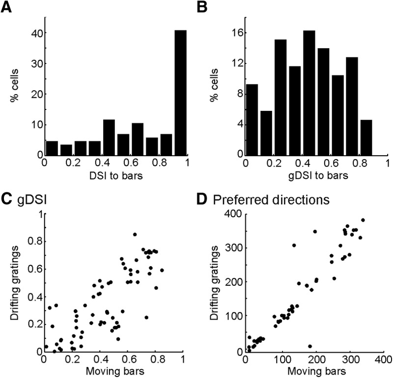
High direction selectivity of sSGS neurons in response to moving bars. A, B, Distributions of DSI (A) and gDSI (B) values of sSGS neurons in response to moving bars. C, D, The gDSI values (C) and preferred directions (D) of the sSGS neurons in response to moving bars match closely with those evoked by the small drifting gratings. Cells that responded to both stimuli were included in C (n = 73 of 172 cells tested), and the selective ones (gDSI > 0.15 to both) were included in D (n = 55).

We next compared the direction selectivity between GAD2⁺ and GAD2⁻ neurons. A recent electrophysiology study showed that the GAD2⁺ neurons in the mouse SGS (presumably most of them, if not all, were from deeper laminae than where we imaged) were rarely DS (Gale and Murphy, 2014). In contrast, we found that, in the sSGS, the GAD2⁺ neurons were also highly selective, with 68% cells having DSI ≥ 0.5 (n = 131 of 192; Fig. 7A). Conversely, an even larger proportion of GAD2⁻ cells had high DSI (80% DSI ≥ 0.5; n = 183 of 230; Fig. 7A), indicating a slightly better selectivity in the putative excitatory neurons. The opposite trend was seen for the OSI distributions, in which a larger proportion of GAD2⁺ cells had OSI ≥ 0.5 (Fig. 7B). However, most importantly, very few cells had high OSI values in both cell types (24% GAD2⁺ and 12% GAD2⁻ cells with OSI ≥ 0.5), indicating that most sSGS neurons were not orientation selective regardless of the cell type. A small but significant difference was observed for the direction tuning width: the GAD2⁻ cells had broader tuning width (mean ± SEM, 121.4° ± 1.5°; median, 122°; n = 180) than the inhibitory GAD2⁺ cells (mean ± SEM, 117.9° ± 1.9°; median, 114°; n = 140; p = 0.002, rank-sum test; Fig. 7C).

Figure 7.

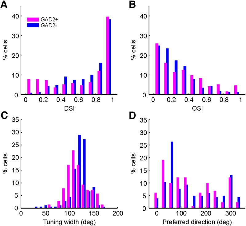
Comparing direction selectivity in excitatory and inhibitory sSGS neurons. A, DSI distribution for GAD2⁺ (magenta) and GAD2⁻ (blue) neurons. B, OSI distribution for these neurons. C, Distribution of tuning widths for both populations. D, Distribution of preferred directions for selective cells (DSI ≥ 0.5) in both populations.

We also observed that sSGS neurons displayed a full range of preferred directions (Fig. 7D), although proportionally more cells preferred 60°, an anterior and upward moving direction. We found that this peak in the distribution was more prominent in the putative excitatory (GAD2⁻) cells (Fig. 7D), but the source or significance of this bias is unknown. We next examined whether the preferred direction of the imaged neurons could be predicted by their RF structure, namely, the asymmetry between the ON and OFF subregions. For cells that responded to both the ON and OFF spots and drifting gratings (n = 317 of 741), we calculated the angle of the vector connecting the OFF to ON centers of each cell and compared it with the preferred direction of the cell. However, no clear trend was observed between the two angles, whether the RF centers were determined by center of mass or after 2D Gaussian fitting (data not shown), suggesting that factors other than RF asymmetry must be involved in generating direction selectivity in sSGS neurons.

Direction selectivity declines with depth in the SGS

The high degree of direction selectivity we revealed for the sSGS neurons is in striking contrast to the results we obtained previously in the mouse SGS across all depths. This difference suggested that different sublaminae of the SGS may contain cells with different degrees of selectivity. Unfortunately, we were not able to test this idea by directly imaging deeper cells, because there were large neuropil signals in deeper regions that severely contaminated the measurement of the selectivity of the individual cells (data not shown). Therefore, we performed single-unit recordings under the same surgical condition as in the two-photon imaging experiments (Fig. 8A) and kept track of the depth of every recorded unit (n = 10 mice, 34 units). The same visual stimuli were used as in the imaging experiments (12 direction drifting gratings within a 30° circular window), except that they were presented at four spatial frequencies (0.02, 0.04, 0.08, and 0.16 cycles/°). Remarkably, the direction selectivity of SGS neurons indeed appeared to decrease with depth (Fig. 8B). The DSI distribution of the entire population of the recorded cells was comparable with what was reported previously (Wang et al., 2010), as well as the mean (0.42 ± 0.06) and median (0.30) DSI (Fig. 8C). However, when separated by depth, cells in the top 100 μm had the highest DSI among the population (mean of 0.69; Fig. 8D). Note that few neurons were sampled at this depth, reflecting the undersampling of superficial neurons in electrophysiology experiments. Cells between 100 and 200 μm had a slightly lower DSI (mean of 0.54), because a significant portion of them was not selective. In contrast, cells deeper than 200 μm had a substantially lower DSI (Fig. 8D). Because the above analysis is confounded by the fact that the depth estimates could vary between mice and/or different electrode penetrations, we further analyzed the data for individual penetrations. In Figure 8E, we connected the neurons that were recorded in the same electrode penetrations to better illustrate the change in DSI. Indeed, when comparing all possible pairs of neurons recorded for each penetration, we found that the mean DSI decreased from 0.57 ± 0.06 for the “more superficial” units to 0.28 ± 0.06 for the “deeper” units of the pairs (Fig. 8F; p = 0.0003, paired t test). Together, our electrophysiology and imaging results demonstrate that highly DS cells are concentrated in the most superficial SGS of the SC, and the degree of selectivity declines with depth.

Figure 8.

Direction selectivity declines with depth in the SGS. A, Single-unit recordings from the SC of anesthetized WT mice during the presentation of spatially restricted drifting gratings. B, Scatter plot showing DSI of the recorded units versus their depth (n = 34 units, 10 mice). C, DSI distribution of the recorded units (mean ± SEM, 0.42 ± 0.06; median, 0.30). D, DSI declines with depth (number of units is shown above each depth bin, values of each bar are means ± SEM). E, Same data as in B but with units recorded sequentially in the same electrode penetration linked together. F, Comparison between all possible pairs of neurons recorded in individual penetrations. The mean DSI decreases from 0.57 ± 0.06 for the more superficial units to 0.28 ± 0.06 for the deeper units (p = 0.0003, paired t test).

Spatial organization of RF properties of sSGS neurons

Finally, simultaneous imaging of dozens of sSGS neurons allowed us to examine their spatial organizations. We first analyzed retinotopic organization of RF positions, separately for ON and OFF subregions. We determined the center of mass of subregions and examined how they varied as a function of physical distance between pairs of cells. On average, cells close to each other had RF centers that were closer in visual space compared with cells farther away (Fig. 9A,D), revealing a retinotopic organization (Cang et al., 2008). However, there were tremendous scatters in this organization at finer scale. In fact, many cells that were next to each other (within 20 μm) had RFs as far apart as 10° (Fig. 9A,B). A similar result was obtained when RF centers were estimated by fitting 2D Gaussians (data not shown). Additionally, we analyzed retinotopic organization of GAD2⁺ and GAD2⁻ neurons separately (data not shown) and observed similar results as in the whole population.

Figure 9.

Spatial organization of RF properties of sSGS neurons. A, Scatter plot showing the distance between the ON subregion centers of pairs of neurons versus the distance between their cell bodies in the SGS. B, Same scatter plots for OFF subregions. C, Bar graphs of the data in A, with values representing means ± SEMs. The number of cell pairs is indicated above each bin. D, Same bar graphs for the data in B. E, Scatter plot showing the difference in preferred directions (ΔPref. Dir.) between pairs of neurons versus the distance between their cell bodies. F, Bar graphs of the data in E. The number of cell pairs is indicated above each bin.

We also examined whether sSGS cells that prefer similar directions are clustered spatially. The difference in preferred directions of pairs of cells was plotted against their physical distance, and no obvious trend was observed (Fig. 9E). In fact, when the data points were binned into increments of 10 μm for the physical distance between cells, a flat distribution was seen for their difference in preferred directions (Fig. 9F). This was also the case when these analyses were separately performed for GAD2⁺ and GAD2⁻ cells (data not shown). In other words, there is no map of directional preference in the most superficial lamina of the mouse SC.

Discussion

In this study, we examined the functional properties of neurons in the sSGS of the mouse SC. We found that the most salient property of the sSGS neurons is their direction selectivity, which is remarkably higher than that of deeper neurons. Interestingly, the high degree of selectivity is seen in both excitatory and inhibitory neurons in the sSGS, with the excitatory neurons tuned slightly more broadly than the inhibitory neurons. We also showed that these neurons have compact RFs that mostly comprise overlapping ON and OFF subregions, mostly consistent with what is known about the RF organization of all SGS neurons. Thus, our results provide critical information for understanding the organization and signal transformation in the early visual system.

Comparison with previous functional studies of the mouse SC

A handful of studies characterized visually evoked response properties of SC neurons in mice (Dräger and Hubel, 1975; Wang et al., 2010; Gale and Murphy, 2014). These studies determined RF organizations, discovered direction and orientation selective responses, and revealed cell-type-specific properties in the mouse SC. However, because all of these studies used electrophysiology, with metal or glass electrodes, the most superficial layer of the SC was likely severely undersampled. Consequently, only indirect comparisons can be made between the current and previous studies. For example, the much higher direction selectivity we observed in the superficial neurons suggested a laminar-specific organization of DS neurons, a hypothesis that was directly confirmed by single-unit recordings in this study. Similarly, we also observed many fewer neurons with good orientation selectivity in the sSGS compared with what was reported previously for the entire SGS (Wang et al., 2010). Thus, it is likely that orientation-selective neurons are more concentrated in the deeper laminae. Furthermore, we found no striking differences between the response properties of GAD2⁺ and GAD2⁻ neurons to flashing squares and drifting gratings. This is in contrast with a recent electrophysiology study showing that the GAD2⁺ neurons (corresponding to horizontal cells in that study) were rarely DS, whereas the excitatory narrow field vertical cells were often so (Gale and Murphy, 2014). This difference between these results is again likely attributable to the fact that the most superficial cells were severely undersampled, if not entirely missed, in that study. Conversely, many of the cells we imaged in this study could very possibly be marginal cells, simply by virtue of their superficial location in the SGS. Indeed, it has been suggested that marginal cells in the hamster SC could be highly DS (Mooney et al., 1985).

A very recent study also used two-photon calcium imaging to examine response properties in the mouse SC and revealed the existence of “orientation columns” (Feinberg and Meister, 2015). In contrast, we find that almost no cells in the superficial SC are truly orientation selective. Instead, these cells are highly DS, and, importantly, they are not clustered according to their preferred directions. A number of technical differences exist between the two studies, including the imaged depth and region, calcium indicators, the anesthetized/awake state of the animal, and whether the cortex was intact. Among them, the difference in imaged depth and region is most intriguing. We imaged the most superficial lamina in the SC, whereas the other study imaged slightly deeper and in more posterior and medial SC, which represents a more peripheral and dorsal visual field. Whether there is a depth and/or region-specific organization of orientation columns in the mouse SC is an interesting possibility that should be answered in future studies.

Direction selectivity in the SC

What might be the source of the high direction selectivity seen in the sSGS? A substantial population of RGCs are DS (Wei and Feller, 2011; Vaney et al., 2012), and most of them project to the SC (Huberman et al., 2010; Dhande and Huberman, 2014). It was shown in mice that the DRD4 RGCs, which are selective for posterior motion, project exclusively into the upper SGS, and, in contrast, the non-DS transient OFF α-RGCs project into the lower SGS (Huberman et al., 2008, 2009). Thus, these results raise an intriguing possibility that the high selectivity we observe in the sSGS neurons could be inherited from the DS RGCs. However, this idea, at least in its simplest form, is not supported by the projection patterns of other subtypes of RGCs. For example, the most numerous type of mouse RGCs, the W3 RGCs, are motion sensitive but not DS (Zhang et al., 2012), and yet, they project to the most superficial lamina in the SC (Kim et al., 2010). Furthermore, individual SGS neurons are estimated to receive inputs from at least four to five RGCs (Chandrasekaran et al., 2007). Finally, the sSGS neurons exhibit a full range of preferred directions, unlike the RGCs, which are selective for cardinal directions. For these reasons, local collicular circuits must be involved in the emergence of the observed response properties in the sSGS. In particular, our finding of selectivity of GAD2⁺ neurons suggests precise and dynamic interactions between the excitatory and inhibitory circuits in transforming direction selectivity in the SGS. It is worth noting that inhibitory neurons in the V1 are less orientation/direction selective than excitatory neurons (Niell and Stryker, 2008; Liu et al., 2009; Kerlin et al., 2010), indicating that the synaptic mechanisms underlying stimulus selectivity are likely different between V1 and SC. Future studies are needed to determine the circuit mechanisms underlying this important transformation in the SC.

Zebrafish is the other model system in which signal transformation from the retina to the SC/OT is studied intensively. It has been shown that subtypes of zebrafish RGCs that prefer different directions project to segregated layers in the tectum and that the tectal neurons with matching preferred directions arborize their dendrites in the corresponding layers (Gabriel et al., 2012; Nikolaou and Meyer, 2012; Lowe et al., 2013; Robles et al., 2013). In other words, the DS retinal inputs could mostly determine the direction preference in at least some of the tectal cells (Gabriel et al., 2012; but see Grama and Engert, 2012). Conversely, new preferred directions emerge in the OT (Hunter et al., 2013), and DS tectal neurons receive inhibitory inputs that are tuned to the null directions (Grama and Engert, 2012), indicating the involvement of local computations in this process. Investigations of the similarities and differences between direction selectivity in mice, zebrafish, and other species will help reach a more complete understanding of functional organization and signal transformation in the visual system.

Dedicated circuits for direction selectivity in the visual system

Many of the DS ganglion cells also project to the dorsal lateral geniculate nucleus (dLGN) in both mice (Dhande and Huberman, 2014) and cats (the “W cells”; Chen et al., 1996). Consistently, a number of studies have reported direction- and orientation-selective responses in the dLGN of mice (Marshel et al., 2012; Piscopo et al., 2013; Scholl et al., 2013; Zhao et al., 2013), cats (Daniels et al., 1977; Vidyasagar and Urbas, 1982; Soodak et al., 1987), and monkeys (Smith et al., 1990; White et al., 1998; Xu et al., 2002; Cheong et al., 2013). In mice, DS cells appear to be more concentrated in the dorsal shell of the dLGN (Marshel et al., 2012; Piscopo et al., 2013), in which some of the DS RGCs terminate (Huberman et al., 2008, 2009). Even more interestingly, the geniculate neurons in the dorsal shell project to layer 1 of the V1, suggesting a dedicated circuit linking DS RGCs to the superficial V1 (Cruz-Martín et al., 2014). In the current study, we reveal for the first time a lamina in the superficial SC that is highly DS, mirroring the finding in the dLGN and V1. This remarkable similarity between the collicular and cortical pathways highlights the evolutionary and behavioral significance of direction selectivity in the visual system.

The dedicated DS circuits in the SC and dLGN V1 could potentially interact with each other via two pathways: the cortico-collicular and colliculo-geniculate pathways. However, the cortico-collicular pathway is an unlikely substrate because it originates from layer 5 in the cortex, in which a DS response is rarely seen (Niell and Stryker, 2008). Conversely, many SC neurons, including those in the sSGS, project directly to the dLGN, as seen in mice (Gale and Murphy, 2014), rats (Lee et al., 2001), hamsters (Mooney et al., 1988), cats (Graham, 1977), tree shrew (Diamond et al., 1991), and monkeys (Harting et al., 1978). Thus, this pathway provides a likely link between the DS sSGS neurons and those in the dLGN.

In summary, we have examined visually evoked responses of neurons in the most superficial lamina of the mouse SC. The high direction selectivity we have revealed in this lamina will guide future investigations to understand the functional organization and signal transformation in the visual system and their underlying circuit mechanisms.

References

- Albano JE, Humphrey AL, Norton TT. Laminar organization of receptive-field properties in tree shrew superior colliculus. J Neurophysiol. 1978;41:1140–1164. doi: 10.1152/jn.1978.41.5.1140. [DOI] [PubMed] [Google Scholar]
- Binns KE, Salt TE. Different roles for GABAA and GABAB receptors in visual processing in the rat superior colliculus. J Physiol. 1997;504:629–639. doi: 10.1111/j.1469-7793.1997.629bd.x. [DOI] [PMC free article] [PubMed] [Google Scholar]
- Brainard DH. The Psychophysics Toolbox. Spat Vis. 1997;10:433–436. doi: 10.1163/156856897X00357. [DOI] [PubMed] [Google Scholar]
- Cang J, Feldheim DA. Developmental mechanisms of topographic map formation and alignment. Annu Rev Neurosci. 2013;36:51–77. doi: 10.1146/annurev-neuro-062012-170341. [DOI] [PubMed] [Google Scholar]
- Cang J, Wang L, Stryker MP, Feldheim DA. Roles of ephrin-as and structured activity in the development of functional maps in the superior colliculus. J Neurosci. 2008;28:11015–11023. doi: 10.1523/JNEUROSCI.2478-08.2008. [DOI] [PMC free article] [PubMed] [Google Scholar]
- Chandrasekaran AR, Shah RD, Crair MC. Developmental homeostasis of mouse retinocollicular synapses. J Neurosci. 2007;27:1746–1755. doi: 10.1523/JNEUROSCI.4383-06.2007. [DOI] [PMC free article] [PubMed] [Google Scholar]
- Chen B, Hu XJ, Pourcho RG. Morphological diversity in terminals of W-type retinal ganglion cells at projection sites in cat brain. Vis Neurosci. 1996;13:449–460. doi: 10.1017/S0952523800008129. [DOI] [PubMed] [Google Scholar]
- Chen H, Zhao Y, Liu M, Feng L, Puyang Z, Yi J, Liang P, Zhang HF, Cang J, Troy JB, Liu X. Progressive degeneration of retinal and superior collicular functions in mice with sustained ocular hypertension. Invest Ophthalmol Vis Sci. 2015;56:1971–1984. doi: 10.1167/iovs.14-15691. [DOI] [PMC free article] [PubMed] [Google Scholar]
- Cheong SK, Tailby C, Solomon SG, Martin PR. Cortical-like receptive fields in the lateral geniculate nucleus of marmoset monkeys. J Neurosci. 2013;33:6864–6876. doi: 10.1523/JNEUROSCI.5208-12.2013. [DOI] [PMC free article] [PubMed] [Google Scholar]
- Cruz-Martín A, El-Danaf RN, Osakada F, Sriram B, Dhande OS, Nguyen PL, Callaway EM, Ghosh A, Huberman AD. A dedicated circuit links direction-selective retinal ganglion cells to the primary visual cortex. Nature. 2014;507:358–361. doi: 10.1038/nature12989. [DOI] [PMC free article] [PubMed] [Google Scholar]
- Daniels JD, Norman JL, Pettigrew JD. Biases for oriented moving bars in lateral geniculate nucleus neurons of normal and stripe-reared cats. Exp Brain Res. 1977;29:155–172. doi: 10.1007/BF00237039. [DOI] [PubMed] [Google Scholar]
- Dhande OS, Huberman AD. Retinal ganglion cell maps in the brain: implications for visual processing. Curr Opin Neurobiol. 2014;24:133–142. doi: 10.1016/j.conb.2013.08.006. [DOI] [PMC free article] [PubMed] [Google Scholar]
- Diamond IT, Conley M, Fitzpatrick D, Raczkowski D. Evidence for separate pathways within the tecto-geniculate projection in the tree shrew. Proc Natl Acad Sci U S A. 1991;88:1315–1319. doi: 10.1073/pnas.88.4.1315. [DOI] [PMC free article] [PubMed] [Google Scholar]
- Dräger UC, Hubel DH. Responses to visual stimulation and relationship between visual, auditory, and somatosensory inputs in mouse superior colliculus. J Neurophysiol. 1975;38:690–713. doi: 10.1152/jn.1975.38.3.690. [DOI] [PubMed] [Google Scholar]
- Elstrott J, Anishchenko A, Greschner M, Sher A, Litke AM, Chichilnisky EJ, Feller MB. Direction selectivity in the retina is established independent of visual experience and cholinergic retinal waves. Neuron. 2008;58:499–506. doi: 10.1016/j.neuron.2008.03.013. [DOI] [PMC free article] [PubMed] [Google Scholar]
- Feinberg EH, Meister M. Orientation columns in the mouse superior colliculus. Nature. 2015;519:229–232. doi: 10.1038/nature14103. [DOI] [PubMed] [Google Scholar]
- Gabriel JP, Trivedi CA, Maurer CM, Ryu S, Bollmann JH. Layer-specific targeting of direction-selective neurons in the zebrafish optic tectum. Neuron. 2012;76:1147–1160. doi: 10.1016/j.neuron.2012.12.003. [DOI] [PubMed] [Google Scholar]
- Gale SD, Murphy GJ. Distinct representation and distribution of visual information by specific cell types in mouse superficial superior colliculus. J Neurosci. 2014;34:13458–13471. doi: 10.1523/JNEUROSCI.2768-14.2014. [DOI] [PMC free article] [PubMed] [Google Scholar]
- Gandhi NJ, Katnani HA. Motor functions of the superior colliculus. Annu Rev Neurosci. 2011;34:205–231. doi: 10.1146/annurev-neuro-061010-113728. [DOI] [PMC free article] [PubMed] [Google Scholar]
- Girman SV, Lund RD. Most superficial sublamina of rat superior colliculus: neuronal response properties and correlates with perceptual figure-ground segregation. J Neurophysiol. 2007;98:161–177. doi: 10.1152/jn.00059.2007. [DOI] [PubMed] [Google Scholar]
- Graham J. An autoradiographic study of the efferent connections of the superior colliculus in the cat. J Comp Neurol. 1977;173:629–654. doi: 10.1002/cne.901730403. [DOI] [PubMed] [Google Scholar]
- Grama A, Engert F. Direction selectivity in the larval zebrafish tectum is mediated by asymmetric inhibition. Front Neural Circuits. 2012;6:59. doi: 10.3389/fncir.2012.00059. [DOI] [PMC free article] [PubMed] [Google Scholar]
- Harting JK, Casagrande VA, Weber JT. The projection of the primate superior colliculus upon the dorsal lateral geniculate nucleus: autoradiographic demonstration of interlaminar distribution of tectogeniculate axons. Brain Res. 1978;150:593–599. doi: 10.1016/0006-8993(78)90822-3. [DOI] [PubMed] [Google Scholar]
- Huberman AD, Manu M, Koch SM, Susman MW, Lutz AB, Ullian EM, Baccus SA, Barres BA. Architecture and activity-mediated refinement of axonal projections from a mosaic of genetically identified retinal ganglion cells. Neuron. 2008;59:425–438. doi: 10.1016/j.neuron.2008.07.018. [DOI] [PMC free article] [PubMed] [Google Scholar]
- Huberman AD, Wei W, Elstrott J, Stafford BK, Feller MB, Barres BA. Genetic identification of an On-Off direction-selective retinal ganglion cell subtype reveals a layer-specific subcortical map of posterior motion. Neuron. 2009;62:327–334. doi: 10.1016/j.neuron.2009.04.014. [DOI] [PMC free article] [PubMed] [Google Scholar]
- Huberman AD, Clandinin TR, Baier H. Molecular and cellular mechanisms of lamina-specific axon targeting. Cold Spring Harb Perspect Biol. 2010;2:a001743. doi: 10.1101/cshperspect.a001743. [DOI] [PMC free article] [PubMed] [Google Scholar]
- Hunter PR, Lowe AS, Thompson ID, Meyer MP. Emergent properties of the optic tectum revealed by population analysis of direction and orientation selectivity. J Neurosci. 2013;33:13940–13945. doi: 10.1523/JNEUROSCI.1493-13.2013. [DOI] [PMC free article] [PubMed] [Google Scholar]
- Kay JN, De la Huerta I, Kim IJ, Zhang Y, Yamagata M, Chu MW, Meister M, Sanes JR. Retinal ganglion cells with distinct directional preferences differ in molecular identity, structure, and central projections. J Neurosci. 2011;31:7753–7762. doi: 10.1523/JNEUROSCI.0907-11.2011. [DOI] [PMC free article] [PubMed] [Google Scholar]
- Kerlin AM, Andermann ML, Berezovskii VK, Reid RC. Broadly tuned response properties of diverse inhibitory neuron subtypes in mouse visual cortex. Neuron. 2010;67:858–871. doi: 10.1016/j.neuron.2010.08.002. [DOI] [PMC free article] [PubMed] [Google Scholar]
- Kim IJ, Zhang Y, Meister M, Sanes JR. Laminar restriction of retinal ganglion cell dendrites and axons: subtype-specific developmental patterns revealed with transgenic markers. J Neurosci. 2010;30:1452–1462. doi: 10.1523/JNEUROSCI.4779-09.2010. [DOI] [PMC free article] [PubMed] [Google Scholar]
- Lee PH, Schmidt M, Hall WC. Excitatory and inhibitory circuitry in the superficial gray layer of the superior colliculus. J Neurosci. 2001;21:8145–8153. doi: 10.1523/JNEUROSCI.21-20-08145.2001. [DOI] [PMC free article] [PubMed] [Google Scholar]
- Liu BH, Li P, Li YT, Sun YJ, Yanagawa Y, Obata K, Zhang LI, Tao HW. Visual receptive field structure of cortical inhibitory neurons revealed by two-photon imaging guided recording. J Neurosci. 2009;29:10520–10532. doi: 10.1523/JNEUROSCI.1915-09.2009. [DOI] [PMC free article] [PubMed] [Google Scholar]
- Liu M, Wang L, Cang J. Different roles of axon guidance cues and patterned spontaneous activity in establishing receptive fields in the mouse superior colliculus. Front Neural Circuits. 2014;8:23. doi: 10.3389/fncir.2014.00023. [DOI] [PMC free article] [PubMed] [Google Scholar]
- Lowe AS, Nikolaou N, Hunter PR, Thompson ID, Meyer MP. A systems-based dissection of retinal inputs to the zebrafish tectum reveals different rules for different functional classes during development. J Neurosci. 2013;33:13946–13956. doi: 10.1523/JNEUROSCI.1866-13.2013. [DOI] [PMC free article] [PubMed] [Google Scholar]
- Madisen L, Zwingman TA, Sunkin SM, Oh SW, Zariwala HA, Gu H, Ng LL, Palmiter RD, Hawrylycz MJ, Jones AR, Lein ES, Zeng H. A robust and high-throughput Cre reporting and characterization system for the whole mouse brain. Nat Neurosci. 2010;13:133–140. doi: 10.1038/nn.2467. [DOI] [PMC free article] [PubMed] [Google Scholar]
- Marshel JH, Kaye AP, Nauhaus I, Callaway EM. Anterior-posterior direction opponency in the superficial mouse lateral geniculate nucleus. Neuron. 2012;76:713–720. doi: 10.1016/j.neuron.2012.09.021. [DOI] [PMC free article] [PubMed] [Google Scholar]
- May PJ. The mammalian superior colliculus: laminar structure and connections. Prog Brain Res. 2006;151:321–378. doi: 10.1016/S0079-6123(05)51011-2. [DOI] [PubMed] [Google Scholar]
- Mazurek M, Kager M, Van Hooser SD. Robust quantification of orientation selectivity and direction selectivity. Front Neural Circuits. 2014;8:92. doi: 10.3389/fncir.2014.00092. [DOI] [PMC free article] [PubMed] [Google Scholar]
- Mooney RD, Klein BG, Rhoades RW. Correlations between the structural and functional characteristics of neurons in the superficial laminae and the hamster's superior colliculus. J Neurosci. 1985;5:2989–3009. doi: 10.1523/JNEUROSCI.05-11-02989.1985. [DOI] [PMC free article] [PubMed] [Google Scholar]
- Mooney RD, Nikoletseas MM, Ruiz SA, Rhoades RW. Receptive-field properties and morphological characteristics of the superior collicular neurons that project to the lateral posterior and dorsal lateral geniculate nuclei in the hamster. J Neurophysiol. 1988;59:1333–1351. doi: 10.1152/jn.1988.59.5.1333. [DOI] [PubMed] [Google Scholar]
- Niell CM, Stryker MP. Highly selective receptive fields in mouse visual cortex. J Neurosci. 2008;28:7520–7536. doi: 10.1523/JNEUROSCI.0623-08.2008. [DOI] [PMC free article] [PubMed] [Google Scholar]
- Nikolaou N, Meyer MP. Imaging circuit formation in zebrafish. Dev Neurobiol. 2012;72:346–357. doi: 10.1002/dneu.20874. [DOI] [PubMed] [Google Scholar]
- Oesch N, Euler T, Taylor WR. Direction-selective dendritic action potentials in rabbit retina. Neuron. 2005;47:739–750. doi: 10.1016/j.neuron.2005.06.036. [DOI] [PubMed] [Google Scholar]
- Piscopo DM, El-Danaf RN, Huberman AD, Niell CM. Diverse visual features encoded in mouse lateral geniculate nucleus. J Neurosci. 2013;33:4642–4656. doi: 10.1523/JNEUROSCI.5187-12.2013. [DOI] [PMC free article] [PubMed] [Google Scholar]
- Robles E, Filosa A, Baier H. Precise lamination of retinal axons generates multiple parallel input pathways in the tectum. J Neurosci. 2013;33:5027–5039. doi: 10.1523/JNEUROSCI.4990-12.2013. [DOI] [PMC free article] [PubMed] [Google Scholar]
- Sarnaik R, Chen H, Liu X, Cang J. Genetic disruption of the On visual pathway affects cortical orientation selectivity and contrast sensitivity in mice. J Neurophysiol. 2014;111:2276–2286. doi: 10.1152/jn.00558.2013. [DOI] [PMC free article] [PubMed] [Google Scholar]
- Schmidt JT. The laminar organization of optic nerve fibres in the tectum of goldfish. Proc R Soc Lond B Biol Sci. 1979;205:287–306. doi: 10.1098/rspb.1979.0066. [DOI] [PubMed] [Google Scholar]
- Scholl B, Tan AY, Corey J, Priebe NJ. Emergence of orientation selectivity in the mammalian visual pathway. J Neurosci. 2013;33:10616–10624. doi: 10.1523/JNEUROSCI.0404-13.2013. [DOI] [PMC free article] [PubMed] [Google Scholar]
- Scott BB, Brody CD, Tank DW. Cellular resolution functional imaging in behaving rats using voluntary head restraint. Neuron. 2013;80:371–384. doi: 10.1016/j.neuron.2013.08.002. [DOI] [PMC free article] [PubMed] [Google Scholar]
- Smith EL, 3rd, Chino YM, Ridder WH, 3rd, Kitagawa K, Langston A. Orientation bias of neurons in the lateral geniculate nucleus of macaque monkeys. Vis Neurosci. 1990;5:525–545. doi: 10.1017/S0952523800000699. [DOI] [PubMed] [Google Scholar]
- Soodak RE, Shapley RM, Kaplan E. Linear mechanism of orientation tuning in the retina and lateral geniculate nucleus of the cat. J Neurophysiol. 1987;58:267–275. doi: 10.1152/jn.1987.58.2.267. [DOI] [PubMed] [Google Scholar]
- Tada M, Takeuchi A, Hashizume M, Kitamura K, Kano M. A highly sensitive fluorescent indicator dye for calcium imaging of neural activity in vitro and in vivo. Eur J Neurosci. 2014;39:1720–1728. doi: 10.1111/ejn.12476. [DOI] [PMC free article] [PubMed] [Google Scholar]
- Taniguchi H, He M, Wu P, Kim S, Paik R, Sugino K, Kvitsani D, Fu Y, Lu J, Lin Y, Miyoshi G, Shima Y, Fishell G, Nelson SB, Huang ZJ. A resource of Cre driver lines for genetic targeting of GABAergic neurons in cerebral cortex. Neuron. 2011;71:995–1013. doi: 10.1016/j.neuron.2011.07.026. [DOI] [PMC free article] [PubMed] [Google Scholar]
- Vaney DI, Sivyer B, Taylor WR. Direction selectivity in the retina: symmetry and asymmetry in structure and function. Nat Rev Neurosci. 2012;13:194–208. doi: 10.1038/nrn3165. [DOI] [PubMed] [Google Scholar]
- Vidyasagar TR, Urbas JV. Orientation sensitivity of cat LGN neurones with and without inputs from visual cortical areas 17 and 18. Exp Brain Res. 1982;46:157–169. doi: 10.1007/BF00237172. [DOI] [PubMed] [Google Scholar]
- Wang L, Sarnaik R, Rangarajan K, Liu X, Cang J. Visual receptive field properties of neurons in the superficial superior colliculus of the mouse. J Neurosci. 2010;30:16573–16584. doi: 10.1523/JNEUROSCI.3305-10.2010. [DOI] [PMC free article] [PubMed] [Google Scholar]
- Wei W, Feller MB. Organization and development of direction-selective circuits in the retina. Trends Neurosci. 2011;34:638–645. doi: 10.1016/j.tins.2011.08.002. [DOI] [PMC free article] [PubMed] [Google Scholar]
- White AJ, Wilder HD, Goodchild AK, Sefton AJ, Martin PR. Segregation of receptive field properties in the lateral geniculate nucleus of a New-World monkey, the marmoset Callithrix jacchus. J Neurophysiol. 1998;80:2063–2076. doi: 10.1152/jn.1998.80.4.2063. [DOI] [PubMed] [Google Scholar]
- Xu X, Ichida J, Shostak Y, Bonds AB, Casagrande VA. Are primate lateral geniculate nucleus (LGN) cells really sensitive to orientation or direction? Vis Neurosci. 2002;19:97–108. doi: 10.1017/s0952523802191097. [DOI] [PubMed] [Google Scholar]
- Zhang Y, Kim IJ, Sanes JR, Meister M. The most numerous ganglion cell type of the mouse retina is a selective feature detector. Proc Natl Acad Sci U S A. 2012;109:E2391–E2398. doi: 10.1073/pnas.1211547109. [DOI] [PMC free article] [PubMed] [Google Scholar]
- Zhao X, Chen H, Liu X, Cang J. Orientation-selective responses in the mouse lateral geniculate nucleus. J Neurosci. 2013;33:12751–12763. doi: 10.1523/JNEUROSCI.0095-13.2013. [DOI] [PMC free article] [PubMed] [Google Scholar]
- Zhao X, Liu M, Cang J. Visual cortex modulates the magnitude but not the selectivity of looming-evoked responses in the superior colliculus of awake mice. Neuron. 2014;84:202–213. doi: 10.1016/j.neuron.2014.08.037. [DOI] [PMC free article] [PubMed] [Google Scholar]