A novel method for testing association of multiple genetic markers with a multinomial trait

Abstract

We developed a multinomial probit model with singular value decomposition for testing a large number of single nucleotide polymorphisms (SNPs) simultaneously, using maximum likelihood estimation and permutation. The method was validated by simulation. We simulated 1000 SNPs, including 9 associated with disease states, and 8 of the 9 were successfully identified. Applying the method to study 32 genes in our Mexican-American samples for association with prediabetes through either impaired glucose tolerance (IGT) or impaired fasting glucose (IFG), we found 3 genes (SORCS1, AMPD1, PPAR) associated with both IGT and IFG, while 5 genes (AMPD2, PRKAA2, C5, TCF7L2, ITR) with the IGT mechanism only and 6 genes (CAPN10, IL4,NOS3, CD14, GCG, SORT1) with the IFG mechanism only. These data suggest that IGT and IFG may indicate different physiological mechanism to prediabetes, via different genetic determinants.

Introduction

Recent technology allows genome-wide association studies (GWAS) to involve a huge number of single nucleotide polymorphisms (SNPs). However, the study samples are often limited. This leads the situation that the number of SNPs (p) is much bigger than available sample (n), which makes the traditional statistical analysis methods unsuitable. Most of current practices analyze one SNP at a time, which create a huge multiple testing problem. In order to analyze all SNPs simultaneously when sample size is much smaller than number of SNPs, we introduced the Iterative Bayesian variable selection (IBVS) method (Kwon et al. 2007) and have successfully applied it to the simulated rheumatoid arthritis data provided by the Genetic Analysis Workshop 15 (GAW15).We later introduced a Bayesian classification with singular value decomposition (BCSVD) method (Kwon et al. 2009) to improve computer’s run-time. Both methods are still limited to dichotomous response variables. We introduce here a multinomial probit model with singular value decomposition (SVD) method for analyzing polychotomous responses in the situation of p ≫ n.We show the validity of the newly developed method by applying it to simulated data set as well as to a real study sample to identify genes contributing to two different mechanisms for prediabetes.

Method and Materials

Multinomial probit model with Singular Value Decomposition

Polychotomous ordinal responses are a type of data that is frequently encountered in common disease studies. A simple example could be found in a study of diabetes, in which subject can be categorized into three groups; normal, prediabetes, and diabetes. Multinomial probit model is commonly utilized to analyze polychotomous categorical responses. The multinomial probit model can be expressed by latent (unobserved) continuous variables associated with categorical responses.

In general, let us assume that the responses y₁, y₂, ⋯, y_n are observed, where y_i takes one of the J ordered categories and θ₀, θ₁, ⋯, θ_J are real numbers of bin boundaries, which satisfy that −∞ = θ₀ ≤ ⋯ ≤ θ_J = ∞. As in Albert and Chib (1993), we denote that z₁, z₂, ⋯, z_n are latent continuous random variables and assume that the latent variable, z_i, associated with a categorical outcome, y_i, can be explained in terms of a underlying linear model and that the observed response y_i has the category j if and only if z_i falls between θ_j−1 and θ_j. Therefore, we can notice that the ordinal probit model is equivalent to the following model.

$$z_i=x_i\beta +{\epsilon }_i,{\epsilon }_i~N(0,1),i=1,\cdots ,n,$$ (1)

$$y_i=j\iff {\theta }_{j-1}<z_i\le {\theta }_j,j=1,\cdots ,J,$$

where x_i is a 1×p vector of the explanatory variables for the i^th sample and β is a p×1 vector of parameters to be estimated. In vector-matrix notation, we can have the multinomial ordinal probit model

$$z=X\beta +\epsilon ,$$ (2)

where z is the n×1 vector of latent variables, X is the n×p matrix of the explanatory variables, β is the p×1 vector of unknown regression coefficients, and ε follows an independent standard multivariate normal distribution, ε ~ N (0, I_n). By applying SVD to the matrix X in (2), we can notice that the matrix can be expressed as follows.

$$X\prime =ADF\prime ,$$ (3)

where A is the p×n singular value factor loading matrix with orthonormal columns so that A′A = I_n, D = diag(d₁,⋯,d_n), the diagonal matrix of positive singular values, ordered as d₁ ≥ ⋯ ≥ d_n > 0, and F is the n × n SVD orthogonal factor matrix with F′F = FF′ =I_n. Therefore, the model in (2) with the SVD of X can be written as follows.

$$z=X\beta +\epsilon =(ADF\prime )\prime \beta +\epsilon =FDA\prime \beta +\epsilon =L\gamma +\epsilon ,$$ (4)

where L = FD and ${\gamma }_{n\times 1}=A_{n\times p}^{\prime }{\beta }_{p\times 1}$. Therefore, the n×1 vector of latent variables, z in (4) has a multivariate normal distribution, i.e., z ~ N (Lγ, I_n).

As shown in (4), we can notice that γ is expressed by a linear combination of the original parameters, β, in (2). Hence, we call γ as super-factors. As mentioned in West et al. (2003), the model in (4) represents a possibly massive dimension reduction from p to n parameters. That is, the regression model with p parameters reduced to that with n parameters derived from the SVD of the design matrix X. Therefore, the statistical inference on the original parameter, β, in (2) turns into the super-factors, γ, in (4).

Model fitting with maximum likelihood estimation

The maximum likelihood estimates of the super-factors, γ, in (4) can be obtained by the iteratively reweighted least squares (IRLS) procedure (Jansen, 1991). The procedure can be briefly described as follows. Let η denote the vector of all model parameters (θ₂, ⋯, θ_J−1, γ₁, ⋯, γ_n−2). Note that θ₁ and θ_J are not included in this vector because their values are assumed to be 0 and ∞, respectively. For example, let J = 4 and n = 15. We define a matrix

$$T_i=\left[\begin{array}{ccc}\hfill 0\hfill & \hfill 0\hfill & \hfill -t_i^{\prime }\hfill \\ \hfill 1\hfill & \hfill 0\hfill & \hfill -t_i^{\prime }\hfill \\ \hfill 0\hfill & \hfill 1\hfill & \hfill -t_i^{\prime }\hfill \end{array}\right]$$ (5)

for i = 1, ⋯, 15. As we see that the vector of new covariates, $t_i^{\prime }$, is preceded by a 3 × 3 identity matrix with the first column excluded corresponding to the imposed constant, θ₁=0. Let S_i be a 4 × 3 matrix,

$$S_i=\left[\begin{array}{ccc}\hfill 1\hfill & \hfill 0\hfill & \hfill 0\hfill \\ \hfill -1\hfill & \hfill 1\hfill & \hfill 0\hfill \\ \hfill 0\hfill & \hfill -1\hfill & \hfill 1\hfill \\ \hfill 0\hfill & \hfill 0\hfill & \hfill -1\hfill \end{array}\right]$$ (6)

and define H_i = diag(f_i1, f_i2, f_i3), where f_ij denotes the derivative of a standard normal distribution at ${\theta }_j-t_i^{\prime }\gamma$. Also, take W_i = diag(p_i), where p_i is the vector of probabilities that each individual falls in each category, and let N be a 15 × 4 matrix of counted responses. Accordingly, we can define the working dependent variable as ω=(ω′₁, ⋯, ω′₁₅)′, where ω_i = S_i H_iT_i + (N_i − p_i), the regressor matrix, $R=(T_1^{\prime }{H}_1{S}_1^{\prime },\cdots ,T_{15}^{\prime }{H}_{15}{S}_{15}^{\prime })\prime$, and the weighted matrix $W=\mathit{\text{diag}}(W_1^{-1},\cdots ,W_{15}^{-1})$. After initialization of all elements in the algorithm, the weighted least square estimate as a solution of a linear equation ω = Rη would be obtained for the (i+1) iteration as

$${\eta }^{i+1}={\eta }^i+{\left(\sum _{i=1}^{15}{T}_i^{\prime }{H}_i^{(i)}{S}_i^{\prime }{W}_i^{-1(i)}{S}_i{H}_i^{(i)}{T}_i\right)}^{-1}\sum _{i=1}^{15}{T}_i^{\prime }{H}_i^{(i)}{S}_i^{\prime }{W}_i^{-1(i)}(N_i-p_i^{(i)})$$ (7)

The matrices ω, R, and W are all recalculated using the current values of η obtained at each least square iteration. This process is performed recursively until changes in the parameter vector η are negligible.

General Solution for the Original Parameters

Since a prior on β determines an prior on γ, the inferences of the original parameter β can be a result of transformation. Due to p ≫ n, the transformation from γ back to β indicates a one-to- many mapping, leading to infinite number of solutions for β. Since the regressor matrix, A, is not square, its inverse must be calculated using the generalized inverse to solve γ = A′β. Let G⁻ denote a generalized inverse of A. As discussed in Graybill (1976, pp34–39), the most general solution to the linear equation can be expressed as

$$\beta =G^{-}\gamma +(I-G^{-}G)h$$ (8)

Where h is some p × 1 vector that can possibly be stochastic or deterministic. Therefore, a unique solution for β from the class of all solutions to the linear equation in (8) can be obtained by the choice of generalized inverse, G⁻ and the characteristic of vector h. As discussed in Graybill (1976), we can achieve the unique solution for β by choosing the generalized inverse of A as G⁻ = A′ since A′A = I.

Selection of the significant genes

Finding significant genes is similar to testing whether the regression coefficient of each SNP is statistically significant, i.e., testing a hypothesis: H₀ : β_i = 0 v.s. H₁ : β_i ≠ 0, i = 1, ⋯, p. However, when p ≫ n, we are unable to perform the test by comparing the test statistic, t = (β̂ − β)/se(β̂), to a critical value, t_1−α/2(n − 2), because of singularity, where β̂ is an estimate of β, α is significant level of the test, se(β̂) is the standard error of β, and n is sample size. As an alternative, we utilized permutation to select significant SNPs. The rationale behind a permutation test is that, under the null hypothesis (H₀ : β_i = 0, i = 1, ⋯, p), the estimate of β obtained from the raw (unshuffled) data is similar to the estimate of β obtained from the shuffled data. Let β̂_i (i = 1, ⋯, p) be the estimate of the i^th SNP effect from the raw data and ${\hat{\beta }}_i^j(j=1,\cdots ,k)$ be the estimate of the i^th SNP effect from the j^th shuffled data. Let us define ${\beta }_i^{d_j}$ as the difference between β̂_i and ${\hat{\beta }}_i^j$, i.e., ${\beta }_i^{d_j}={\hat{\beta }}_i-{\hat{\beta }}_i^j$. Then,

$${\mathrm{\Lambda }}_i=\frac{{\overline{\beta }}_i^d}{se({\overline{\beta }}_i^d)}~N(0,1),i=1,\cdots ,p,$$ (9)

where ${\overline{\beta }}_i^d$ is the sample mean of ${\beta }_i^{d_j}’\mathrm{s}$, j = 1, ⋯, k, i.e. ${\overline{\beta }}_i^d=\frac{1}{k}{\sum }_{j=1}^k{\beta }_i^{d_j}$ and $\mathrm{s}\mathrm{e}({\overline{\beta }}_i^d)$ is the standard error of ${\overline{\beta }}_i^d$. Under the null hypothesis, the statistic Λ_i defined in (14) follows standard normal distribution when k is large. p-value for rejecting the null hypothesis and the rank of each Λ_i can be utilized to select significant SNPs.

Application of the multinomial probit model with SVD

Simulated multinomial data

To evaluate the validity of the multinomial probit model with SVD for polychotomous ordinal responses, we simulated 30 samples and 1000 SNPs, with 9 out of the 1000 SNPs (every 100^th SNP, except the last one) contribute to disease status. We assumed that there are 3 disease development stages and a dominant genetic model for each of the 9 disease associated SNPs. Therefore, we would expect 9 strong signals corresponding to each of the 9 disease associated SNPs when applying the multinomial probit model with SVD to this data.

Mexican-American Coronary Artery Disease (MACAD) study

The Study population consists of probands who are Mexican American aged between 45 and 75 with coronary artery disease: Spouses of probands, adult offspring (≥ 18) and their spouses. For the offspring generation, we performed Oral Glucose Tolerance Test and genotyped 132 SNPs in 32 genes selected for a prior relationship to insulin physiology. Table 1 summarized the list of 132 SNPs in 32 genes. The goal of this study was to identify genes affecting the development of impaired glucose tolerance (IGT) and/or impaired fasting glucose(IFG). Impaired glucose tolerance (IGT) was defined as a 2hr glucose level between 140 and 199 mg/dl; Impaired fasting glucose (IFG) defined as a fasting glucose level between 100 and 125 mg/dl. In order to identify and compare genes affecting the development of IGT and/or IFG, we generated two study samples, D1 and D2 (Figure 1). Each has 3 disease stages: D1) both 2hr and fasting glucoses normal (N/N) (n₁=60), IGT only (IGT/N) (n₂=31) and IGT and IFG (IGT/IFG) (n₃=15); D2) both 2hr and fasting glucoses normal (N/N) (n₁=60), IFG only (N/IFG) $(n_2^{\prime }=34)$ and IGT and IFG (IGT/IFG) (n₃=15).

Table 1.

List of 132 SNPs in the 32 candidate genes.

Gene	SNP	Gene	SNP	Gene	SNP	Gene	SNP
LPL	m7315	AMPD2	rs12046107	NOS3	rs1800779		rs1800874
	m8292		rs865774		rs3918226	MS4A2	rs574700
	m8393		rs568686		rs1799983		rs1441586
	m8852		rs523786	NPPARS	rs5063		rs2583471
	m9040	PRKAG3	rs650898	PPARS	rs5065		rs2070970
	m9712		rs16859382	SCNN1	rs5742912	FEM1B	rs10152450
CAPN	n44		rs6436094		rs2228576		rs11636081
	n43		rs692243	ADRB2	rs1042713		rs7172340
	n56	PRKAA2	rs11206887		rs1042714	GCG	rs13429709
	n63		rs2051040	CRP	rs3091244		uw012629
SORCS	rs2249022		rs2143749	TCF7L2	m11196181		rs6732914
	rs1537919		rs2746349		m17747324		rs7581952
	rs7897974		rs857155		m7901695		rs5645
	rs1530248	CRP	rs1130864		m11196187		rs13001107
	rs11193190		rs1800947		m7077039	ITR	rs6492722
	rs2243454		rs2808630		m11196199	LPIN	rs11524
	rs4390282		rs3093062		m17685538	PPARα	rs135549
	rs10736189	C5	rs25681m		m12255372		rs135547
	rs10748924		rs2416811	AMPD1	rs926938		rs63382
	rs10509818		rs2159776		1q12x		rs1800206
	rs10748932	IL4	rs2070874		rs2010899		rs82789
	rs11193188		rs2227284		rs2268701	PTPN1	rs941798
	rs1251753		rs2072130		1p48l		rs3787345
	rs1269918		rs3024622		rs2268698		rs754118
	rs1322005	IL6	rs2069832		rs2268697		rs2282147
	rs1538417		rs2069849		rs3789627		rs718050
	rs2788677	C5	rs17611		rs743041		rs3787348
	rs607437	IL4R	rs2243250		rs761755	SORCS3	rs813756
	rs685316		rs1805010		rs6679869		rs1670008
	rs7067660		rs1805015		rs6701427	SORT1	rs4970843
	rs7086426		rs1801275	CD14	rs4914		rs1278664
	rs821994	IL6	rs1800796	CCR5	rs1799988		rs11581665
	rs822000		rs1800795		rs2254089		rs1149175

Figure 1.

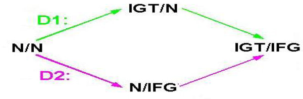
Two Study Samples: D1. Both 2hr and fasting glucoses normal (N/N)-IGT only (IGT/N)-IGT and IFG (IGT/IFG) and D2. Both 2hr and fasting glucoses normal (N/N), IFG only (N/IFG), and IGT and IFG (IGT/IFG)

Results

Simulated Multinomial Data

Figure 2 shows the result of estimate of parameters. There are 8 strong signals, showing that 8 out of the 9 disease associated SNPs were successfully identified by the method, even though some nosies are around each signals. This showed that multinomial probit model with SVD can be reliably used to analyze large scale association data when p ≫ n for polychotomous ordinal responses.

Figure 2.

Estimate of parameters in the simulated data

Mexican-American Coronary Artery Disease (MACAD) study

We analyzed two data sets generated from a subsample of subjects recruited through a coronary artery disease proband in the Mexican-American Coronary Artery Disease Project. Figure 3 shows the result of estimate of parameters, which are β′s in (1), using the MLE method and p-values of 132 SNPs in 32 genes to test each SNP effect for the data set D1. P-values are were calculated from (9). At significance level 0.05, which is 1.3 (= −log₁₀(0.05)), we identified that 8 genes out of the 32 candidate genes that were associated with D1. Figure 4 gives the parameter estimates and −log₁₀(p − value) of 132SNPs for data set D2. At significance level 0.05, 9 genes out of the 32 candidate genes were associated with D2. These results suggested that SNPs in 3 genes (SORCS1, AMPD, PPARα) were associated with both D1 and D2; SNPs in 5 genes (AMPD2, PRKAA2, C5, TCF7L2, ITR) were associated with D1 only; SNPs in 6 genes (CAPN, IL4, NOS3, CD14, GCG, SORT1) were associated with D2 only (Table 2). These results suggest that IGT and IFG may indicate different pathways to diabetes, with different genetic determinants. Multinomial Probit model with SVD can be utilized to identify associated markers with disease development when multi-disease stages are conside

Figure 3.

Genes for IGT/IFG through IGT pathway

Figure 4.

Genes for IGT/IFG through IFG pathway

Table 2.

Genes identified as significant for D1 and D2.

Study sample	Genes selected
both IGT and IGF	SORCS1 (Sorcs receptor 1) AMPD1 (Adenosine monophosphate deaminase-1) PPARα (Peroxisome proliferators-activated receptor-α)
only	AMPD2 (Adenosine monophosphate deaminase-2) PRKAA2 (Protein kinase AMP-activated catalytic α2) C5 (Complement component 5) TCF7L2 (Transcription factor 7-like 2)
only	CAPN10 (Calpain 10) IL4 (Interleukin 4) NOS3 (Nitric oxide synthase 3) CD14 (Monocyte differentiation antigen cd14) GCG (Glucagon) SORT1 (Sortilin)

References

- Albert J, Chib S. Bayesian analysis of binary and polychotomous response data. Journal of American Statistical Association. 1993;88:669–679. [Google Scholar]
- Anderson M, Legendre P. An empirical comparison of permutation methods for tests of partial regression coefficients in a linear model. Journal of Statistical Computation and Simulation. 1999;62:271–303. [Google Scholar]
- Croiseau P, Cordell H. Analysis of North American Rheumatoid Arthritis Consortium data using penalized logistic regression approaches. Genetic Analysis Work-shop. 2008;16 doi: 10.1186/1753-6561-3-s7-s61. [DOI] [PMC free article] [PubMed] [Google Scholar]
- Chib S, Greenberg E. Analysis of Multivariate Probit Models. Biometrika. 1998;85:347–361. [Google Scholar]
- Gelfand A. Model determination using sampling-based methods. In: Gilks, Richardson, Spiegelhalter, editors. Markov china Monte Carlo in Practice. London, England: Chapman & Hall; 1996. pp. 145–161. [Google Scholar]
- George E, McCulloch R. Variable selection via Gibbs sampling. Journal of American Statistical Association. 1993;88:881–889. [Google Scholar]
- George E, McCulloch R. Approached for Bayesian variable selection. Statistica Sinica. 1993;7:339–373. [Google Scholar]
- Graybill F. Theory and Application of the Linear Model. Belmont, California: Duxbury Press; 1976. [Google Scholar]
- Jansen J. Fitting regression models to ordinal data. Biometrical Journal. 1991;33:807–815. [Google Scholar]
- Johnson V, Albert J. Ordinal Data Models. New York: Springer-Verlag; 1999. [Google Scholar]
- Kennedy P. Randomization tests in econometrics. Journal of Business and Economic Statistics. 1995;13:85–94. [Google Scholar]
- Kwon S, Wang D, Guo X. Application of an iterative Bayesian variable selection method in a genome-wide association study of rheumatoid arthritis. BMC proceedings. 2007 doi: 10.1186/1753-6561-1-s1-s109. [DOI] [PMC free article] [PubMed] [Google Scholar]
- McCullagh P. Regression models for ordinal data (with discussion) Journal of the Royal Statistical Society. Series B. 1980;42:109–142. [Google Scholar]
- Meier L, van de Geer S, Buhlman P. The group lasso for logistic regression. Journal of the Royal Statistical Society. 2008;70:53–71. [Google Scholar]
- Sha N, Vannucci M, Tadesse M, Brown P, Dragoni I, Davies N, Roberts T, Contestabile A, Salmon M, Buckley C, Falciani F. Bayesian variable selection in multinomial probit models to identify molecular signatures of disease stage. Biometrics. 2004;60:812–819. doi: 10.1111/j.0006-341X.2004.00233.x. [DOI] [PubMed] [Google Scholar]
- West M. Bayesian factor regression models in the large p, small n paradigm. Bayesian Statistics. 2003;7:723–732. [Google Scholar]