Electron Tomography of Yeast Cells

Introduction

Electron microscopy (EM) is a useful method for the study of yeast cells and is complementary to a genetic analysis. EM provides high-resolution structure data about wild type cells and can document structural defects in mutant strains^1,2. A number of EM techniques have been used to study the complex three-dimensional (3-D) arrangements of organelles in yeast. Examples include the use of freeze fracture replicas to reveal the surface topology of nuclear envelopes and cytoplasmic membrane systems^3,4,5, as well as the use of serial sections to reconstruct entire mating factor-arrested cells⁶, to describe the 3-D geometry of the mitotic spindle^7,8, and to document the 3-D distribution of nuclear pore complexes in wild type⁹ and mutant strains¹⁰. More recently, electron tomography has been used to describe the 3-D architecture of the yeast spindle pole body (SPB)¹¹ and forming mitotic spindles¹².

Electron tomography has proven to be a useful method for obtaining 3-D structure data to describe complex cellular substructures¹³. Tomography is based on a series of tilted images, usually collected from a comparatively thick (0.2-1μm) section or from isolated organelles, to generate a 3-D reconstruction using back projection algorithms¹⁴. This method is like a ‘CAT’ scan of a cell, where the result is a computer-generated reconstruction that can be computationally sectioned and viewed in any orientation at 5-10 nm spatial resolution. In contrast to serial section reconstruction where multiple thin (50-70nm) sections have been used to reconstruct cellular objects that extend over many micrometers (e.g. an anaphase mitotic spindle^15,16) tomography is best suited for structures whose dimensions change significantly, such that standard thin sections cannot reconstruct them accurately. Tomographic reconstruction permits the viewing of computer-generated ‘slices’ that are much thinner than could ever be cut physically with a microtome. This approach is therefore ideal for structures that have a complex 3-D geometry, such as arrays of cytoskeletal elements or convoluted membrane systems. In this chapter, we describe the steps necessary to prepare yeast cells for tomography and provide examples that illustrate the procedures for calculating tomographic reconstructions of organelles in situ and of whole cell profiles.

Equipment requirements and software packages

Microscope requirements

An intermediate voltage microscope (IVEM) operating at 200-400 kV or high voltage electron microscope (HVEM) operating at 750-1000kV, is necessary for collecting tilt series data from thick (0.2μm – 1μm) sections. The increased accelerating voltages of these microscopes reduces the scattering cross-section of the beam electrons, allowing them to penetrate the thicker specimens with less inelastic and plural scattering, thus improving image quality. This feature of high energy beams becomes particularly important when the specimen is tilted up to 60-70°, where the section thickness doubles or nearly triples, relative to the electron beam. More limited questions can be addressed by tomography using thinner sections (e.g. 50nm) with lower voltage EMs. In the United States, there are several NIH-supported National Research Resources that have the expertise and equipment to do routine tomography (Boulder Laboratory for 3-D Fine Structure, University of Colorado, Boulder, http://bio3d.colorado.edu; Wadsworth Center, Albany, N.Y., http://www.wadsworth.org; and the National Center for Microscopy and Imaging Research, University of California, San Diego, http://www-ncmir.ucsd.edu). These facilities are set up to help investigators collect and analyze data, and the reader is encouraged to contact the web pages of these facilities to obtain more information.

Equipment for digital image capture

The images can be collected digitally using either standard EM film or a high resolution charge coupled device (CCD) camera. If the images are collected on film, the film optical density must be scanned and converted to digital form for further analysis. Our method has been to place the negative on a motor-controlled light box and digitize the image with a high-quality CCD camera ¹⁷. Generally, a pixel size corresponding to 1-3 nm at the plane of the specimen is suitable for tomographic studies of yeast. If images are collected directly in digital form on the microscope, the pixel size may need to be smaller than when working from film because of the limited resolution of microscope CCD cameras.

Software packages

There are several software packages available to generate, display, and analyze tomographic data. Our laboratory has developed the IMOD software package, which contains all of the programs needed for calculating tomograms, displaying the reconstructions, and modeling image data ¹⁸. The Imod viewing program uses the MRC image file format and is convenient because multiple images can be stored in a single file, or ‘image stack’. The Imod viewing program allows an investigator to read in an image stack and then step or “movie” through the series of images. The program can also be used to model features within a data set and to display 3-D models. In addition, the package contains roughly 85 programs for 3-D analysis, including measurement and display-enhancement features. The IMOD package was originally developed to run on a Unix platform using SGI computers with 24 bit graphics, but has now been ported to run on a PC under Linux. Executable versions of the IMOD programs are freely available on our website (http://bio3d.colorado.edu), and the details of their use will be discussed in examples given below. The web site also provides a detailed guide for tomographic reconstruction that describes how to use specific programs and how to trouble-shoot problems that arise. Once the IMOD package is installed, the operator can run the programs with a series of command files that contain all of the information needed to initiate the programs that align tilt series data and calculate a tomographic reconstruction.

Similar software packages have been developed and made available, including the SPIDER, WEB, and STERECON packages developed at the Wadsworth Center, Albany N.Y.^19,20,21, the SUPRIM package developed at the University of Texas²², and several image processing and display software packages developed and used at the National Center for Microscopy and Image Research in San Diego ^23,24,25. Although there are operational differences in the software packages used to generate, display, and analyze tomographic reconstructions, the basic steps required to create a tomographic reconstruction are similar in all of them; these are outlined in Table 1. The details of each step and examples illustrating their use in yeast cell biology are discussed below.

Table 1.

Steps Involved in Creating Tomographic Reconstructions of Yeast

Specimen preparation for electron tomography

The purpose of tomographic study in yeasts or in any cell is to obtain high quality 3-D fine structural data, therefore, the initial fixation of the cells for electron microscopy is a critical step. Artifacts introduced by poor fixation will have a serious negative effect on the quality of the final reconstruction. We have found that high pressure freezing, followed by freeze-substitution, results in excellent preservation of cellular fine structure. The reader is referred to the chapter by McDonald in this volume for details of the method²⁶. The specimens imaged in this chapter were prepared for EM by high pressure freezing, followed by freeze-substitution in 3% glutaraldehyde and 0.1% uranyl acetate in acetone at 90°C for three days, then low-temperature embedded in Lowicryl HM20. Because this method results in a pellet of cells that are embedded in random orientations, it is advisable to cut serial sections in order to find suitable cell profiles or images of specific organelles. Serial thick (200-500 nm) sections are cut using a microtome and collected onto slot grids coated with 0.7% formvar. Because of the increased thickness of the sections used for tomography compared to standard electron microscopy, the samples must be post stained for longer periods of time. We have found that staining with 2% uranyl acetate in 70% methanol for 10 minutes followed by Reynold’s lead citrate for 5 minutes provides good contrast and stain penetration.

The final step in preparing specimens for electron tomography is the addition of colloidal gold particles to each surface of the section. This is done by placing a drop (~20μl) of 10 or 15 nm colloidal gold suspension (BBI International) on top of the grid for several minutes, dipping the grid in dH₂0, then repeating the procedure on the other side of the grid. The gold particles that adhere to the two surfaces will serve as fiducial markers for subsequent image alignment²⁷. A thin film of carbon may also be evaporated on the grids to stabilize the samples during electron microscopy.

Data collection

The thick sections can first be imaged in a conventional transmission microscope operating at 100 kV to find sections that contain specific organelles or to identify a cell in a particular stage of the growth and division cycle. Low magnification overview maps can be collected to facilitate finding the particular cell in the higher voltage microscopes, where contrast is greatly reduced. For data collection in an IVEM or HVEM, the grid is placed in a tilting specimen holder and the goniometer of the microscope stage is adjusted to permit eucentric tilting by adjusting the tilt axis so it lies in the plane of the specimen and passes through the region of interest. This adjustment is useful because it decreases the amount of time the microscope operator spends focusing and positioning the specimen during data collection. The specimen is then tilted to 60 or 70 degrees, and serial tilted views are collected to the opposite extreme tilt at intervals of 1-2°, depending on the resolution desired in the tomogram. For dual axis tomography, the grid is rotated in the specimen holder by 90° and a second tilt series is acquired.

A microscope equipped to collect a tilt series automatically is very useful for facilitating image capture and increasing throughput. Several laboratories have developed procedures for microscope automation and papers describing their use have been published^28,29,30,31. The Boulder 3-D lab has developed a program for semi-automated data collection procedure that drives Gatan’s Digital Micrograph software to collect images from a 1024 × 1024 pixel CCD camera. The program also controls essential microscope functions such as focus and tilt, so it can collect single frame or montaged images of large cellular profiles and store the serial images in MRC format. Generally, a magnification of 12,000 on the microscope, corresponding to a pixel size of 1.4 nm is used.

Alignment of serial tilts and tomographic reconstruction

Our standard method for alignment of serial images first begins by reading the image stack containing the raw, serial tilts into Imod, and one section at low tilt is displayed. The positions of 10-20 gold particles are then marked by placing a model point in the center of each gold particle (Figure 1a, open circles). An automatic bead-tracking program is then used to track and model the corresponding images of each gold particle through all of the images of the tilt series. The resulting computer-generated ‘fiducial’ model is then edited manually to correct any small errors in the placement of the model point or any gaps in the data set. Figure 1a and Video Sequence 1a (available on our web site, http://bio3d.colorado.edu/MIE.html) show images of a 200 nm thick section through a small yeast bud with the positions of 16 gold particles marked (Figure 1a, open circles; Video Sequence 1a, green circles). Gold particles that are attached to the top and bottom surfaces of the section appear to move in opposite directions relative to each other as one movies through the tilt series (Video Sequence 1a).

Figure 1.

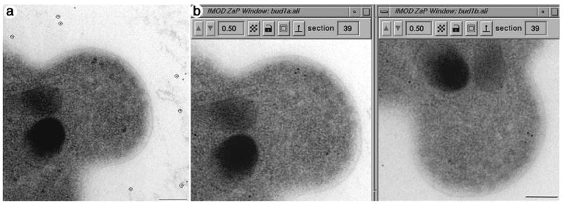
Serial, tilted views of a single thick section are used as the raw data for tomographic reconstructions. Figure 1a shows an image of a 200nm thick section through a portion of an emerging bud from a diploid yeast cell. Gold particles placed on the top and bottom surfaces of the section are used as fiducial markers for alignment because their position can be located in every view. Approximately 10-20 gold particles are modeled (open circles around the 15 nm gold, Figure 1a). Images are collected every 1.5° over a ± 60 or ± 70° range. For best results, a dual-axis approach is applied, where the grid is rotated 90° and a second tilt series is acquired (Figure 5b). Supplementary video material for Figures 1a and b can be found at our website, http://bio3d.colorado.edu/MIE.html. Video sequence 1a shows 78 serial tilted views of the 250 nm thick section shown in Figure 1a with green model points marking the position of 16 gold particles used as markers for alignment. Video sequence 1b shows the complete, aligned serial tilt series from each axis. Note there is little fine structure resolved in any one view because there is so much cellular material superimposed in a 200nm thick section. This is particularly true at the high tilts, where section thickness has doubled relative to the electron beam axis. Bar = 200nm.

The serial, tilted images are then aligned by the program, Tiltalign, which uses the positions of the gold particles and a least squares approach to solve for tilt angles, shifts, rotations, magnification changes, and section distortion³². The transforms created by Tiltalign are then applied to the image data, resulting in an aligned stack. Figure 1b shows images from aligned stacks of a small yeast bud taken from a tilt series obtained from tilting around the Y (vertical) axis and the same bud rotated 90° and then tilted again about the vertical axis. Video sequence 1b (available on our web site, http://bio3d.colorado.edu/MIE.html) shows movies of the aligned tilt series containing 78 serially, tilted views separated by 1.5° over a ± 60° range. Note that little fine structure can be resolved in these thick sections in any one view because there is so much cellular material superimposed within the volume of the thick section.

The next step is to compute the tomographic reconstruction, using the density information in the aligned tilt series. The program we use employs an R*-weighted back projection algorithm³³. This step is the most computationally intensive in the whole process and results in reconstructions that can be quite large (>500 megabytes). Moreover, the reconstructed section is often not flat or centered improperly within the volume of the data set. To save time, it is useful first to run the program on a small (10 pixel) slice of the aligned stack to identify any adjustments that need to be made to make the reconstruction flat and centered, and to fit within the smallest volume possible. The procedures in the IMOD package include command files to generate 3 samples of the reconstruction and analyze them to determine the shifts and rotations that must be made to keep the section level and centered. They also measure the thickness of the reconstruction. With these adjustments, the final reconstruction is calculated from the full-sized, aligned tilt series.

For electron tomography of sectioned biological material, there is a limitation in the range of tilts that one can collect, generally up to ±60 or ±70°. This is due to several factors such as the specimen support grid occluding the image at high tilt, the physical stops in the microscope that prevent the specimen rod from hitting pole pieces and apertures, and the difficulty in obtaining well-focused images of thick sections at tilt angles greater than 60-70 degrees. These limitations in the range of tilt angles that can be sampled results in a missing wedge of information, which leads to a decrease in resolution of the tomogram.

Several laboratories have worked to overcome or at least minimize the impact of this missing wedge. One approach is conical tilting³⁴ and others include combining information from tilt series taken about two orthogonal axes, also known as ‘dual-axis tomography’^35,36. Our laboratory has developed an improved method of dual-axis tomography, where tomograms are computed separately from tilt series taken about two orthogonal axes, then the two tomograms are aligned to each other and combined to achieve a single tomogram ³⁷. This dual-axis approach results in resolution that is almost isotropic, which is valuable, especially for extended features that are perpendicular to a tilt axis.

Figure 2 shows an example of a budding yeast cell that contains duplicated, side-by-side SPBs and associated nuclear and cytoplasmic microtubules. The tomogram calculated from tilt series collected about the first axis shows good resolution of nuclear and cytoplasmic microtubules (Figure 2a, arrows), yet the microtubules are poorly resolved (Figure 2b, arrows) in the tomogram calculated from the tilt series collected after rotating the grid 90°. Similarly, features that are perpendicular to the cytoplasmic microtubules, such as the SPB, are better resolved in the tomogram calculated from the second tilt series (Figure 2a and b, arrowhead). Figure 2c shows the combined tomogram where both microtubules and SPBs are well resolved. This illustrates that the dual axis approach is the method of choice for a tomographic study of complex biological material.

Figure 2.

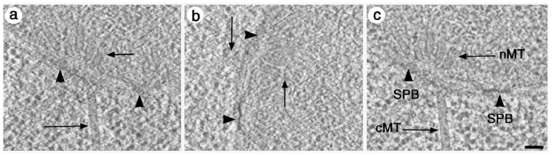
The benefits of dual axis tomography. Slices taken from tomograms of duplicated side-by-side SPBs from tilt series collected about two orthogonal axes (Figure 2a and 2b) can be very different. The cytoplasmic and nuclear microtubules (Figure 2a, arrows) are well resolved in the tilt series taken about the first axis, yet the SPBs are poorly resolved (Figure 2a, arrowhead). When the grid is rotated 90° and a second tilt series is collected, the SPBs in the resulting tomogram are well resolved (Figure 2b, arrowheads) yet the microtubules show up poorly. The combined tomogram (Figure 2c) shows features at all orientations well resolved. Bar = 50nm.

Modeling image data

Cellular features in the dual axis tomogram can be modeled, and the resulting 3-D model displayed for study and analysis (Figure 3, and supplementary video material available at our website, http://bio3d.colorado.edu/MIE.html). The tomographic slices shown in Figures 3a and 3b are 1.4 nm thick and are viewed parallel to the plane of the original 200 nm section. Organelles such as secretory vesicles (sv), a mitochondrion (M), endoplasmic reticulum (ER), and a portion of the vacuole (Vc) can be resolved clearly in these slices (Figure 3a). Video sequence 3a is a movie of 55, serial, 1.4 nm thick tomographic slices from the top surface of the original thick section, through to its bottom surface. The 3-D relationships of organelles and their arrangement in the bud are particularly evident when moving slice-by-slice through the entire tomographic volume.

Figure 3.

Modeling organelles of an emerging yeast bud. (3a) 1.4 nm tomographic slice through a portion of a small yeast bud. The tomographic slice is viewed parallel to the plane of the original 200 nm thick section. Organelles such as ER, mitochondrion, vacuole and secretory vesicles are clearly resolved. Bar = 200 nm. (3b) Organelles were modeled by depositing model points along the membranes of the plasma membrane (green), ER (yellow), a mitochondrion (light blue), and a portion of the vacuole (purple) forming contours that defined the boundaries of the organelle in any given slice. Vesicles were modeled by depositing a single point on the tomographic slice that contained the maximum diameter of the vesicle. Such points were displayed as scattered points with a sphere size set for the particular kind of vesicle (blue, red spheres). (3c,d). 3-D model created by surface rendering of contour data. The plasma membrane of the bud is shown in green and encapsulates a bud filled with secretory vesicles (blue, red), ER (yellow), a mitochondrion (light blue) and a portion of the vacuole (purple). (3d) Individual objects can be turned on or off to display the 3-D relationship of particular organelles to each other, such as the vesicles (blue, red) relative to ER (yellow). Supplementary video material for Figures 3a-d can be found at our web site, http://bio3d.colorado.edu/MIE.html. Video sequence 3a shows a movie of 55 serial 1.4 nm thick tomographic slices. The bud is filled with organelles that can be clearly resolved. In Video sequence 3b, modeling software was used to place model points to define contours of specific organelles. The convoluted nature of the ER (yellow) in this bud is particularly evident when moving through the tomographic volume. Video sequences 3c and 3d are rotating 3-D models of the organelles modeled in this tomographic reconstruction.

Objects of interest are modeled separately and are made up of a series of stacked contours or a set of scattered points. In the example shown in Figure 3b, the different organelles within the cell are represented by different graphic objects, each designated by a unique color. The boundaries of each organelle are traced by hand to create a contour, and a new contour is created on each successive tomographic slice in which the organelle can be found. Video Sequence 3b is a movie of 55 serial 1.4 nm tomographic slices with model contours marking the positions of the plasma membrane (green), the ER (yellow), a mitochondrion (light blue), a portion of the vacuole (pink), and two classes of vesicles that have different sizes (marked blue and red). The elaborate membrane system of the ER (yellow) in this emerging bud would be difficult to model with accuracy using other reconstruction methods, because the contours of the membrane change significantly over very short distances.

Once the contours of all the objects of interest are traced, the resulting model can then be viewed as a 3-D projection of the entire modeled volume and modified for viewing in several ways. The contour data can be ‘meshed’ to create a skin over each modeled object (Figure 3c and 3d and Video Sequence 3c and 3d). Small, regular objects like vesicles can also be displayed as spheres whose diameters are set to correspond to the diameter of the object of interest (Figure 3b-d, red and blue vesicles). The full model may be displayed to show all objects (Figure 3c) or only selected objects, facilitating the study of the 3-D relationships among a particular subset of the objects in the model (Figure 3d, ER relative to the vesicles). Video Sequences 3c and 3d, show the 3-D models rotating 360° about a vertical axis. They illustrate the polarity of the organelle distribution in the emerging bud.

Finally, quantitative information such as the number of particular objects, their surface areas, volumes, length distributions, and nearest neighbor distances, can be determined from the model contour data using companion programs such as Imodinfo. This information is useful for testing ideas about structural relationships among organelles within the cell in 3-D.

Tomographic reconstructions of larger cellular volumes

When tomography is used to study large intracellular compartments, such as endomembrane systems or cytoskeletal arrays, it is often best to reconstruct as large a volume as possible. To image large cellular areas with high, uniform resolution, multiple image frames or ‘montages’ must be assembled. Such images of large cellular areas or even entire cell profiles, can also be used for tomographic analysis, using minor modifications of the procedures outlined above. First, the edges of the montaged pieces must be ‘blended’ to reconcile any differences in intensity or position between the pixels that overlap between adjacent frames of the images. Figure 4a shows an image of a montaged cell captured using four, 1024 × 1024 pixel frames, corresponding to an area of 4.3μm × 4.3μm from this small-budded yeast cell. Note that there are small differences in image intensity between the four frames, yet the edges between the frames show gradual transitions.

Figure 4.

Tomographic reconstruction of a large cellular area. (a) Four adjacent image frames (1024 × 1024 pixels each) were collected using a pixel size of 2.1 nm with automated image capture software developed in our laboratory. The total area captured equals 4.3 × 4.3 μm. The pixels that overlapped between adjacent frames were blended, the tilt series was aligned using local alignment methods, and a tomogram calculated. Bar = 200 nm (b) The resulting tomogram shows fine structure detail when panned at high magnification. Individual microtubules in the nucleus (nMT) and cytoplasm (cMT) can be detected as well vesicles (v), endoplasmic reticulum (ER), and the double membrane of the nuclear envelope. Bar = 200 nm. (c) The Imod ‘slicer’ tool was used to extract a piece of image data that contained an oblique cytoplasmic microtubule (white arrow). The orientation of the slice was then rotated 9° about the horizontal axis to bring the entire length of the microtubule into one view. Bar = 50 nm. Supplementary video material for Figures 4a and 4b are available on our web site, http://bio3d.colorado.edu/MIE.html) Video sequence 4a is a movie of 78 aligned serial tilt series from the blended image stack. Video sequences 4b and 4b’ are movies of the resulting tomographic reconstruction shown at low magnification (Video sequence 4b) and viewed at higher magnification with image viewing software (Video sequence 4b’). Note that the trajectory of the oblique cytoplasmic microtubule (marked by the white arrow in Figure 4b) can be followed to the bud neck when stepping through the tomographic volume.

When imaging comparatively large areas (>2μm × 2μm), we have found that there are distortions in the resulting images that are not homogeneous over the area sampled. These distortions are likely due to differential thinning and/or shrinkage of the section under the action of the electron beam, or from slight bending of the section on the formvar film, all of which can lead to a poor global alignment. To solve this problem, the tilt alignment program has been modified to use a subset of fiducial markers to solve for local alignments, which are then taken into account by the back projection program. Video sequence 4a shows a movie of an aligned, blended tilt series. The nucleus, bud, and most of the cell is represented in this montage.

Details of the cellular fine structure can be clearly resolved in tomograms calculated from montaged images when panning the tomogram at higher magnification. For example, the double membrane of the nuclear envelope, the nuclear microtubules of the mitotic spindle (nMT), vesicles (v) and cytoplasmic microtubules (cMT) are clearly resolved (Figure 4b,c). Supplementary video material for Figure 4 shows movies of 40, 2.11nm tomographic slices of the whole montaged cell (Video sequence 4b) and viewed with a zoom tool at higher magnification to show an area of the cell that contains the mitotic spindle and cytoplasmic microtubules (Video sequence 4b’). The trajectory of the oblique cytoplasmic microtubule identified in Figure 4b (cMT, arrow) can be followed up to the bud neck in this movie. The high density of spindle microtubules in the nucleus is also evident.

The Imod software developed in our laboratory provides an additional tool, the ‘slicer’ window, which allows an investigator to rotate the orientation of a particular tomographic slice to view a structure from any chosen angle. For example, the tomographic slice shown in Figure 4b contains an oblique cytoplasmic microtubule (cMT). The orientation of the tomographic slice was then rotated 9° about the horizontal axis to sample the entire microtubule axis in one view (Figure 4c, cMT). The close associations between vesicles and this cMT can be appreciated more easily when viewed in this manner.

Higher resolution, dual-axis tomograms can also be calculated from montaged images and can yield a tremendous amount of structural data from larger cellular volumes. Figure 5a and b and video sequences 5a and b show tomographic slices from a 1.5 × 2.9 μm area of a cell that has just undergone cytokinesis. Portions of the two resulting cells are shown at the top and bottom of the image, respectively. The cells are filled with ribosomes, secretory vesicles, ER and Golgi. Electron-dense cell wall material can be seen deposited between the adjacent cells. When the tomogram is viewed at higher magnification (Figure 5b), the details of the electron-dense secretory vesicles (SV), a budded cisterna of the Golgi membrane (G), and the plasma membranes of the two adjacent cells (arrows) can be clearly resolved. When moving slice-by-slice through the tomographic volume (Video sequence 5b) vesicles of different sizes can be detected as well as the contours of ER and Golgi that are in close proximity to the electron-dense secretory granules.

Figure 5.

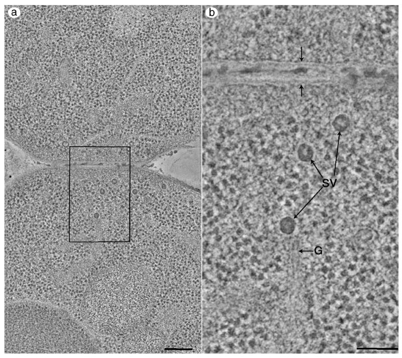
Dual axis tomography of montaged images. (a) 1.4 nm thick tomographic slice through a cell that has just undergone cytokinesis. Portions of the two resulting cells are at the top and bottom of the image, respectively. The total cellular area represented in the tomogram is 1.5 × 2.9μm. Bar = 200 nm (b) The tomogram can be viewed at higher magnification using a zoom tool in the image viewing software (boxed area in Figure 5a) revealing a tremendous amount of cellular fine structure. Individual, electron-dense secretory vesicles (SV), a Golgi cisterna containing a coated bud (G) and the individual leaflets of the plasma membranes of the adjacent cells can be seen (arrows). Bar = 100 nm. The 3-D fine structure is best appreciated when viewing supplementary video material (found at our web site, http://bio3d.colorado.edu/MIE.html). Video sequences 5a and 5b show movies of 50, 1.4 nm thick tomographic slices through the volumes represented in Figures 5a and 5b. The cells are filled with ribosomes and membrane systems such as ER and Golgi can be detected. Secretory vesicles filled with electron-dense material similar to the material deposited between the plasma membranes of the adjacent cells can be detected.

Finally, even larger volumes can be reconstructed by calculating tomograms from serial thick sections^38,39. The serial tomograms can then be knitted together to obtain high resolution structure information about large cellular volumes. This procedure has been recently applied in a tomographic study describing the reconstruction of a 3 × 4 × 1.2 μm region of the Golgi apparatus in a pancreatic β cell⁴⁰. The potential disadvantage of this method is the apparent loss (up to 25- 40nm) of material that occurs between serial thick sections, which sometimes makes alignment and modeling across these gaps difficult.

Conclusion

Due to recent technical advances in specimen preparation and image analysis, electron tomography is now a routine method with which to study the 3-D fine structure of cellular subsystems. Tomographic reconstruction results in 3-D image data with resolutions that significantly exceed those obtained by serial section reconstruction. In addition, the technique enables one to slice and view an organelle in many orientations, giving a more comprehensive understanding of complex biological structures. When combined with a mutant analysis of yeast, tomography will likely provide new structural insights to help define structure-function relationships in this organism.