Collaborative regression

Abstract

We consider the scenario where one observes an outcome variable and sets of features from multiple assays, all measured on the same set of samples. One approach that has been proposed for dealing with these type of data is “sparse multiple canonical correlation analysis” (sparse mCCA). All of the current sparse mCCA techniques are biconvex and thus have no guarantees about reaching a global optimum. We propose a method for performing sparse supervised canonical correlation analysis (sparse sCCA), a specific case of sparse mCCA when one of the datasets is a vector. Our proposal for sparse sCCA is convex and thus does not face the same difficulties as the other methods. We derive efficient algorithms for this problem that can be implemented with off the shelf solvers, and illustrate their use on simulated and real data.

1. Introduction

The problem of combining data from multiple assays is an important topic in modern biostatistics. For many studies, the researchers have more data than they know how to handle. For example, a researcher studying cancer outcomes may have both gene expression and copy number data for a set of patients. Should that researcher use both types of predictors in their analysis? Should any care be given to distinguish the fact that these predictors are coming from different assays and may have differing meanings? If the researcher needs to make future predictions based on only gene expression, is there a way that having copy number data in a training set can help those predictions? All of these are important questions that are still up for debate.

In this paper, we propose a method for this problem called collaborative regression (CoRe), a form of sparse supervised canonical correlation analysis (sCCA). In Section 2, we define CoRe and characterize its solution. This involves explicit closed form solutions for the unpenalized algorithm, as well as a discussion of some useful convex penalties that can be applied.

We look at using CoRe in a sparse sCCA framework in Section 3, including a simulation study where we compare CoRe to one of the leading competitors. Then, in Section 4 we explore the possibility of using CoRe in a prediction framework. While this may seem like an intuitive use case, simulations suggest that CoRe is not able to improve prediction error even over methods that do not take advantage of the secondary dataset. Finally, we show how the penalized version can be applied to a real biological dataset in Section 6 with a comparison with sparse CCA. In the supplementary material available at Biostatistics online, we explore how to efficiently solve the convex optimization problem given by the penalized form of the algorithm.

2. Collaborative regression

CoRe is a tool designed for the scenario where there are groups of covariates that can be naturally partitioned and a response variable. Let us assume that we have observed instances of covariates and a response. We can partition the covariates into two matrices, and , that are and , respectively. The response values are stored in a vector, , of length . Then, CoRe finds the and that minimize the following objective function:

(2.1)

where and are parameters that control the relative importance of the three terms in the objective. This objective function seems natural for the multiple dataset situation. It suggests that we want to make predictions of based on or , but we will penalize ourselves based on how different the predictions are. Essentially, the goal is to uncover a signal that is common to , , and .

Consider trying to maximize the objective function (2.1). The optimal solution, and will satisfy the following first-order conditions:

(2.2)

(2.3)

By substituting for and solving, we can find a closed form solution for :

(2.4)

In the above, we have assumed that and are nonsingular. Assuming they are, and none of the parameters are zero, then that guarantees the invertibility of

Note that and will generally be nonsingular in the classical case where .

2.1. Infinite series solution

Another way to characterize the optimal solution to the objective function (2.1) is as an infinite series. Instead of solving for after substituting, consider instead what would happen if we just continued substituting for or on the RHS. Then, we get an infinite series representation of . Let be the matrix that performs orthogonal projection onto the column space of (and let be defined similarly). Then we can also write as:

(2.5)

If we let

Then

(2.6)

Looking at the infinite expansion can help build some understanding of what CoRe actually does. We note that , so essentially CoRe is equivalent to regressing the weighted average of the 's on . Those 's trace out the path of successive projections onto the column space of and . As the column spaces of and are affine, it is known from Projection onto Convex sets that the sequence will converge to the projection of onto the intersection of those two spaces (Murray and Von Neumann, 1937). In the case where the columns of and are linearly independent, will eventually converge to 0. Thus, CoRe is basically shrinking towards the part that can be explained by both and .

Additionally, we get some picture as to how the parameters affect the solution. acts in large part to control the amount of shrinkage imposed on , while does the same for .

2.2. Penalized collaborative regression

One nice aspect of the objective function (2.1) is that it is convex. This means that the problem can still be easily solved through convex optimization techniques if we add convex penalty functions to the objective (Boyd and Vandenberghe, 2004). Additionally, as we will see in supplementary material available at Biostatistics online, these penalized versions of CoRe can often be implemented with out of the box solvers.

We can define a penalized version of CoRe as finding the minimizer of the following objective:

(2.7)

where and are convex penalty functions. Note that some of the convex penalties that may warrant use include:

• The lasso: is an penalty on , namely . The lasso penalty is known to introduce sparsity into for sufficiently high values of .

• The ridge: is a squared penalty on , namely . Ridge penalties help to smooth the estimate of to ensure nonsingularity. This can be especially important in the high-dimensional case where is known to be singular.

• The fused lasso: . The fused lasso will help to ensure that is piecewise constant. This can be helpful if there is reason to believe that the predictors can be sorted in a meaningful manner (as with copy number data).

In addition to the convex penalties above, situations may also call for linear combinations of those penalties. For example, the lasso and ridge penalties are often combined to find sparse coefficients for predictors that are highly correlated. The lasso and fused lasso are often combined to find sparse and piecewise constant coefficient vectors. In supplementary material available at Biostatistics online, we discuss solving the penalized version of CoRe efficiently in the case where the penalty terms are lasso penalties.

3. Supervised canonical correlation analysis

Canonical correlation analysis (CCA) is a data analysis technique that dates back to Hotelling (1936). Given two sets of centered variables, and , the goal of CCA is to find linear combinations of and that are maximally correlated. Mathematically, CCA performs the following constrained optimization problem:

(3.1)

In this form, it is possible to derive a closed form solution for CCA using matrix decomposition techniques. Namely, will be the eigenvector corresponding to the largest eigenvalue of . A similar expression can be found for by switching the roles of and .

CCA might be a useful tool for finding a signal that is common to both and , but there is no guarantee that the discovered signal will also be associated with . To approach this issue, a generalization of CCA called multiple canonical correlation analysis (mCCA) was developed. mCCA allows for 2 datasets and seeks to find a signal that is common to all of the datasets. The case we have, where the third dataset is a vector, can be thought of as a special case of mCCA that we will call sCCA.

There are many techniques that approach the mCCA problem. Most of them focus on optimizing a function of the correlations between the various datasets. Gifi (1990) provides an overview of many of the suggestions that have been made for this problem. One example of an optimization problem that people call mCCA is based on trying to maximize the sum of the correlations:

(3.2)

The optimization problem above is multiconvex as long as each of the is nonsingular. This means that a local optimum can be found by iteratively maximizing over each given the current values of the rest of the coefficients.

3.1. Sparse sCCA

For high-dimensional problems (where for at least one ), several issues emerge when doing sCCA. First, the constraints given in equation (3.2) are no longer strictly convex constraints because is necessarily singular for at least one . This means that the problem cannot be as easily solved by an iterative algorithm.

One approach that some people take to this problem is to add a ridge penalty on the coefficients. As with ridge regression, adding a ridge penalty will effectively replace with ( being the identity matrix), which will then be nonsingular. This means that the mCCA problem in equation (3.2) can be solved by adding a ridge penalty. Examples of works where people have pursued this method include Leurgans and others (1993). Another approach is pursued by Witten and Tibshirani (2009) where is replaced by in order to ensure strict convexity of the constraints.

Now, even after adjusting to make sure that the constraints (or penalties in the Lagrange form) are convex, there is still another issue that the high-dimensional regime adds. For many high-dimensional problems, the goal is to do some sort of variables selection. After all, it is much more useful for a biologist to uncover 30 genes or pathways that are particularly important in a process than it is to uncover 30 000 coefficient values that are all fairly noisy. Another way to state that is that we want to find coefficients that are sparse (mostly 0). There has been a lot of work in sparse statistical methods following the introduction of the lasso (Tibshirani, 1996). Witten and Tibshirani (2009) offer the following optimization problem to perform sparse mCCA:

where the can be chosen to impose the desired level of sparsity on each coefficient vector. Note that further convex constraints (or penalties) can be added to the above such as the fused lasso or non-negativity constraints. As with the other methods, this problem is multiconvex and can be solved through an iterative algorithm. This method, MultiCCA, was implemented by Witten and others (2013) in the R package PMA.

Note however that a multiconvex problem may be particularly hard to solve in a high-dimensional space. While we know the algorithm will converge to a local optimum, we would ideally like to find the global optimum. For a low-dimensional space, this can be mostly resolved by doing multiple starts from random points in the coefficient space. With enough starts, we believe that we can search the space sufficiently well that our best local optimum is at least close to globally optimum. This logic breaks down in high-dimensional spaces because it is impossible to sufficiently search the space without exponentially many starting points. This means that while the previously discussed methods for Sparse mCCA have outputs, we will not know whether those outputs are even optimizing the objective function in high dimensions. In Section 5.3, we present a simulation that supports this suspicion.

Another option to perform sparse high-dimensional sCCA was suggested by Witten and Tibshirani (2009). They suggest that a method of supervision similar to Bair and others (2006) can be used: before doing a fit, all of the variables are screened against . Only the ones that have correlation above some threshold will be passed along to a CCA model. This method can also be used to add a supervised component to any of the methods that can be used to perform CCA. The main issue with this approach is that it does the supervision in a way that is completely univariate. While univariate analyses can be interesting, they tend to do a relatively poor job in uncovering multivariate signal (Wasserman and Roeder, 2009).

3.2. Penalized collaborative regression as sparse sCCA

Consider one of the three terms from our objective function:

(3.3)

Now let's compare that with the following version of the CCA problem:

(3.4)

We can convert the CCA problem from its bounded form into the Lagrange form as follows:

(3.5)

where and are chosen appropriately to enforce the unit variance constraint. In this way, CCA can also be characterized as a penalized optimization problem. Thus, CoRe with is very similar to doing a sum of correlations mCCA as in the equation (3.2), with the exception that we have picked the penalties that allow for convexity instead of the penalties that correspond to unit variance.

Now it is worth noting that an unenviable fact about the penalty used in equation (3.3) is that it results in the minimum being achieved by setting all of the coefficients equal to zero. Fortunately, CoRe avoids this issue because of the two terms involving .

As discussed in Section 2.2 one of the advantages of CoRe is the simplicity with which convex penalties can be added to the objective function. Thus, it is easy to convert CoRe into a form that is appropriate for sparse sCCA by adding penalties just as in Witten and Tibshirani (2009).

In Section 5.2, we conduct a simulation to compare the performance of CoRe and MultiCCA. CoRe outperforms MultiCCA in that simulation except in the recovery of signal variables at high levels of recall. In particular, it seems that MultiCCA often became trapped in the local optima described in the previous section. Thus, CoRe with seems to be the best available option to perform sparse sCCA.

4. Using CoRe for prediction

Another potentially appealing use of CoRe is when we want to make predictions of for future cases based only on the variables in ; the variables in are only available in the training set. Can the information contained in be used to help identify the correct direction in ? There are many practical situations in which this framework might be useful. For example, maybe it is much more costly to gather data with a lower amount of noise. Alternatively, it could be that some data is not accessible until after the fact; autopsy results may be very helpful in identifying different types of brain tumors, but it is hard to use that information to help current patients.

CoRe seems like it provides a natural way in which to perform a regression with additional variables present only in the training set. Basically, it is saying that we want our future predictions to agree with what we would have predicted given . In this framework, CoRe is similar to “preconditioning” as defined by Paul and others (2008). Instead of preconditioning on and then fitting the regression, we are simultaneously doing the preconditioning and fitting.

Looking at the infinite series solution in Section 2.1 it is clear that performing CoRe is similar to doing ordinary regression after shrinking . If that shrinkage on is done in such a way that it reduces noise, we may ultimately expect ourselves to do better in estimating the correct . We investigate this in a simulation in Section 5.1 and ultimately conclude that CoRe is not well suited for this task.

5. Simulations

We decided to generate data from a factor model to test CoRe. A factor model seems natural for this problem, and is a simple way to create correlations between , , and . Another reason the factor model was appealing is because it is relatively easy to analyze, and given and it is easy to compute statistics like the expected prediction error or the correlations between linear combinations of the variables. More concretely, given values for parameters , and , we generate data according to the following method:

1. distributed MVN(0,),

2. distributed iid MVN(0,) for ,

3. ,

4. distributed iid MVN(0,) for ,

5. ,

6. For :

   1. distributed iid MVN(0, ),
   2. with distributed N(0, ),
   3. with distributed MVN(0, ),
   4. with distributed MVN(0, ).

7. , , and .

Thus, steps 1–5 generate the factors () and step 6 generates the loadings () and noise.

5.1. Regression or supervised CCA

The first simulation was designed to test the effectiveness of CoRe in the two problems that seem natural, sCCA, and prediction. We generated a set of factors from the model with , , , . Then, for each of 80 repetitions, we generated loadings and noise before fitting a range of models. CoRe was fit with and a variety of values of . Additionally, at each level of we fit models with a range of ridge penalties. Ridge regression models were also fit, which corresponds to . To evaluate the success of the fits, we looked at prediction error based on using just relative to ordinary regression as well as the sum correlation. Here, by sum correlation, we mean , where is a future observation (corresponding to making another pass through step 6).

The results of the simulation, in Figure 1, shed some light on the effectiveness of using CoRe to improve a regression of on . First, we note that ridge regression with optimal complexity outperforms CoRe at any choice of and penalty for this particular problem. At first, this might seem surprising given the fact that CoRe gets the advantage of using and ridge regression does not. When looking at the sum correlation though, we see that CoRe outperforms ridge. This suggests that the reason CoRe is doing worse on predicting is because it is focusing on the distance between and instead of just the typical RSS. Essentially, CoRe is giving up a little of the fits involving in order to get a higher correlation between and . Thus, it seems that CoRe is more naturally suited for the sCCA problem.

Fig. 1.

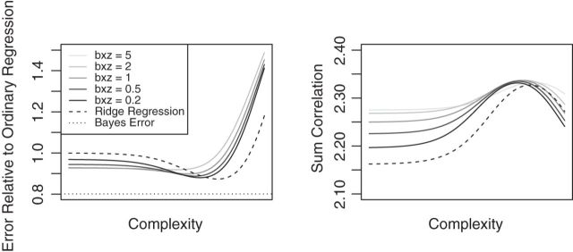
Results of a simulation study to test the effectiveness of CoRe with penalty in a prediction framework. Here, the points all the way to the left correspond to no penalty and the penalty increases (simpler models) as we move right along the -axis. The first plot shows prediction error for making future predictions based on only. The second plot shows the theoretical sum correlation. Values have been averaged over 80 repetitions. As we can see, while CoRe outperforms ordinary regression with no penalty in terms of prediction error (the far left of the first plot), Ridge regression achieves a lower minimum. The second plot helps illuminate the reason; CoRe does a better job of maximizing the sum correlation, so it is sacrificing some of the correlation between and in order to get a larger correlation between and .

5.2. Comparison with MultiCCA

To compare CoRe against a competing algorithm for sparse sCCA, we generated data from the above model with , , , , . Then, we added variables to both and that were generated from new factors that have no effect of . These variables act as confounding variables that reflect an effect we do not want to uncover. This could correspond to a batch effect in the measurements, or maybe some other underlying difference among the sampled patients. Finally, we added another columns to and that were just independent Gaussian to act as null predictors. We ran both CoRe with a lasso penalty and Witten's MultiCCA from the PMA package with an constraint each over a range of parameter values. This process was repeated 80 times with new loadings and noise each time but the same factors. Figure 2 shows the average (over repetitions) theoretical sum correlation for future observations, as well as the recovery of true predictors, against a range of nonzero coefficients that corresponds to a range of penalty parameters.

Fig. 2.

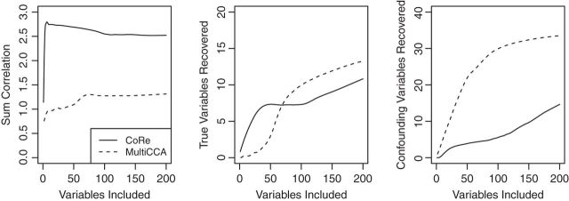
Results of a simulation to compare CoRe and MultiCCA in performing sparse supervised mCCA. For each repetition, a dataset with , is created. For both and , of the predictors are confounding variables and of the predictors are true variables (the rest are null). Confounding variables are the ones that share a signal between and , but not . The true variables share a signal between all three datasets. Values have been averaged over repetitions. MultiCCA is much more susceptible to picking up the confounding variables, and thus has a much harder time achieving high correlations. Interestingly, while CoRe finds many more true variables at first, after or so included variables MultiCCA starts finding more.

From the results, we can see that CoRe does a much better job of finding coefficients that have high sum correlation. MultiCCA seems to get caught in the trap set by the confounding variables, which makes it harder to raise the sum correlation much (a perfect correlation between and with no relation to ). Interestingly, while MultiCCA does worse than CoRe on recovery of true variables for the first 70 or so variables added, it seems to do a better job of recovering true variables after that point. It is unclear what exactly is causing that transition in this problem.

5.3. MultiCCA random starts

Finally, we generated some data to test the extent to which MultiCCA gets caught in local optima. These datasets have , , , . For , 500, 2000, and 5000, we generated a single dataset with and then ran MultiCCA from 1000 random (uniform on the unit sphere) start locations. Figure 3 shows histograms of the resulting objective values. The vertical lines correspond to the default starting point of MultiCCA, and a starting point that is based on a penalized CoRe solution. As we can see, there are many local optima that emerge especially in higher dimensions. One interesting aspect of the results is that the CoRe starts typically end up in a better solution than the default starts provided by the MultiCCA function.

Fig. 3.

Result of a simulation to see how close the locally optimal solutions to MultiCCA end up to the global optimum. Histograms of objective values of MultiCCA from random starts. As we can see, the random starts end up at a variety of local optima, and using the results of CoRe as a starting point often outperforms the default start which is based on an singular value decomposition. In each case, .

6. Real data example

To demonstrate the applicability of penalized CoRe, we also ran it on a high-dimensional biological dataset. We used a neoadjuvant breast cancer dataset that was provided by our collaborators in the Division of Oncology at the Stanford University School of Medicine. Details about the origins of the data can be found at ClinicalTrials.gov using the identifier NCT00813956. This dataset consists of patients who underwent a particular breast cancer treatment. Before treatment, the patients had measurements taken on their gene expression as well as copy number variation. In all, after some preprocessing, there were gene expression measurements per patient and copy number variation measurements. Additionally, each patient was given a RCB score 6 months after treatment that corresponds to how effective the treatment was. The RCB score is a composite of various metrics on the tumor: primary tumor bed area, overall % cellularity, diameter of largest axillary metastasis, etc.

The goal of the analysis is to select a set of gene expression measurements that are highly correlated with a particular pattern of copy number variation gains or losses. That said, we are only interested in sets that also correlate with the RCB value. As such, it is the perfect opportunity to employ CoRe.

Due to computational limitations and issues with noise in the underlying measurements, some further pre-processing was done to the data. First, the gene expression measurements were screened by their variance across the subjects. Only the top gene expression genes were kept. For the copy number variation measurements, we needed to account for the fact that for each patient the copy number variation measurements are highly autocorrelated because they had already been run through a circular binary segmentation algorithm—a change point algorithm used to smooth copy number variation data (Olshen and others, 2004). We use a fused lasso penalty to help correct for the fact that we do not really have gene level measurements. However, doing fused lasso solves can be very slow for large , so we took consecutive triples of the copy number variation measurements and averaged them. This reduced the number of copy number variation measurements to . Our new and matrices were centered and scaled, and then CoRe on the dataset with and the following parameters and penalty terms:

We searched a grid of in order to find a solution with 50 nonzero coefficients in each set of variables. This corresponds roughly with the number of genes a collaborator thought she would be able to reasonably examine for plausible connections. The penalty terms on were chosen in a way that the selected coefficients had a manageable number of nonzero segments. The resulting vector can be seen in Figure 4.

Fig. 4.

The resulting vector of coefficients for the copy number variation data from running CoRe on the RCB dataset. Regions with positive coefficients (amplification associated with higher RCB) are darker and appear above the line. Regions with negative coefficients are lighter and appear below the line. The size of the bars are proportional to the coefficient values. Missing chromosomes had no nonzero coefficients. The piece-wise constant nature of the coefficient vector is due to the use of a fused lasso.

In addition to fitting CoRe, we also fit a penalized version of CCA to show the importance of supervision. We used the CCA function from Witten's PMA package for R. This allows us to impose an penalty on and a fused lasso on . Parameters were chosen to give similar sparsity patterns as the CoRe fits (number of nonzero coefficients in and number of nonzero sections in ).

If we evaluate the correlations of , , and , we see a predictable pattern emerge. While the CCA method got a slightly higher correlation between and (0.78 compared with 0.79), CoRe attained a much higher sum of correlations (2.28 compared with 1.02). These results make sense because CoRe specifically targets the correlation between and in the direction of . It is worth noting that this comparison is being made on training data and only for the purposes of illustrating the difference between CCA and sCCA. In practice, correlations should be estimated by cross validation or with a withheld test set.

This highlights the real use case for sCCA. While a researcher can always do CCA with this data, it can be difficult to interpret the output and there are no guarantees that any of the canonical correlates will line up with a quantity of interest. In this case, it is difficult to interpret the CCA output because while we know the two linear combinations of covariates move together, we have no intuition on what the quantity actually represents; it could be some response to the treatment, a batch effect, or some combination of many different effects. With sCCA, we are guaranteed to be finding linear combinations that also comove with .

7. Discussion

In this paper, we introduced a new model called collaborative regression, which can be used in settings where one has two sets of predictors and a response variable for a set of observations. We explored the possibility of using CoRe in a prediction framework, but concluded that it was not particularly well suited for that task.

We then discussed the problem of sparse sCCA, which is an increasingly interesting problem for biostatistics. While current approaches to sCCA are biconvex and do not necessarily lend themselves to a sparse generalization, CoRe does not suffer from those same issues. We used several simulations and real data to explore both the issues of biconvexity in high dimensions, as well as the performance of CoRe.

As we saw in Section 6, often practitioners may want to apply CCA or penalized CCA in the case where they have partitioned covariates. This can lead to results that are difficult to interpret. By using CoRe with and some supervising , we can do a supervised version of the CCA problem. These results should be easier to interpret because we already have a sense of what the underlying variation means (it is variation in the direction of ).

This paper already explored some of the benefits of having a method that can be implemented with existing solvers, but there are further benefits as well. Recently, there has been a lot of research into finding valid -values for the lasso and related models. Examples of this work include Lockhart and others (2014) and Taylor and others (2013). This work could be extended to provide significance measures for the variables selected by CoRe.

References

- Bair E., Hastie T., Paul D., Tibshirani R. (2006). Prediction by supervised principal components. Journal of the American Statistical Association 101, 119–137. [Google Scholar]
- Boyd S., Vandenberghe L. (2004). Convex Optimization. Cambridge, UK: Cambridge University Press. [Google Scholar]
- Gifi A. (1990). Nonlinear Multivariate Analysis. Chichester: Wiley. [Google Scholar]
- Hotelling H. (1936). Relations between two sets of variates. Biometrika 28(3/4), 321–377. [Google Scholar]
- Leurgans S. E., Moyeed R. A., Silverman B. W. (1993). Canonical correlation analysis when the data are curves. Journal of the Royal Statistical Society. Series B (Methodological) 55(3), 725–740. [Google Scholar]
- Lockhart R., Taylor J., Tibshirani R., Tibshirani R. (2014). A significance test for the lasso. Annals of Statistics 42(2), 413–468. [DOI] [PMC free article] [PubMed] [Google Scholar]
- Murray F. J., Von Neumann J. (1937). On rings of operators. II. Transactions of the American Mathematical Society 41(2), 208–248. [Google Scholar]
- Olshen A. B., Venkatraman E. S., Lucito R., Wigler M. (2004). Circular binary segmentation for the analysis of array-based DNA copy number data. Biostatistics 5(4), 557–572. [DOI] [PubMed] [Google Scholar]
- Paul D., Bair E., Hastie T., Tibshirani R. (2008). “Pre-conditioning” for feature selection and regression in high-dimensional problems. Annals of Statistics 36(4), 1595–1618. [Google Scholar]
- Taylor J., Loftus J., Tibshirani R. (2013). Tests in adaptive regression via the Kac-rice formula. arXiv:1308.3020; submitted.
- Tibshirani R. (1996). Regression shrinkage and selection via the lasso. Journal of the Royal Statistical Society, Series B 58, 267–288. [Google Scholar]
- Wasserman L., Roeder K. (2009). High dimensional variable selection. Annals of Statistics 37(5A), 2178. [DOI] [PMC free article] [PubMed] [Google Scholar]
- Witten D. M., Tibshirani R. (2009). Extensions of sparse canonical correlation analysis, with application to genomic data. Statistical Applications in Genetics and Molecular Biology 8(1), Article 28. [DOI] [PMC free article] [PubMed] [Google Scholar]
- Witten D., Tibshirani R., Gross S., Narasimhan B., Witten M. D. (2013). Package “PMA”. Genetics and Molecular Biology 8(1), 28. [Google Scholar]
Associated Data
This section collects any data citations, data availability statements, or supplementary materials included in this article.