Optimal Thresholding of Classifiers to Maximize F1 Measure

Abstract

This paper provides new insight into maximizing F1 measures in the context of binary classification and also in the context of multilabel classification. The harmonic mean of precision and recall, the F1 measure is widely used to evaluate the success of a binary classifier when one class is rare. Micro average, macro average, and per instance average F1 measures are used in multilabel classification. For any classifier that produces a real-valued output, we derive the relationship between the best achievable F1 value and the decision-making threshold that achieves this optimum. As a special case, if the classifier outputs are well-calibrated conditional probabilities, then the optimal threshold is half the optimal F1 value. As another special case, if the classifier is completely uninformative, then the optimal behavior is to classify all examples as positive. When the actual prevalence of positive examples is low, this behavior can be undesirable. As a case study, we discuss the results, which can be surprising, of maximizing F1 when predicting 26,853 labels for Medline documents.

1 Introduction

Performance measures are useful for comparing the quality of predictions across systems. Some commonly used measures for binary classification are accuracy, precision, recall, F1 measure, and Jaccard index [15]. Multilabel classification is an extension of binary classification that is currently an area of active research in supervised machine learning [18]. Micro averaging, macro averaging, and per instance averaging are three commonly used variations of F1 measure used in the multilabel setting. In general, macro averaging increases the impact on final score of performance on rare labels, while per instance averaging increases the importance of performing well on each example [17]. In this paper, we present theoretical and experimental results on the properties of the F1 measure. For concreteness, the results are given specifically for the F1 measure and its multilabel variants. However, the results can be generalized to Fβ measures for β ≠ 1.

Two approaches exist for optimizing performance on the F1 measure. Structured loss minimization incorporates the performance measure into the loss function and then optimizes during training. In contrast, plug-in rules convert the numerical outputs of classifiers into optimal predictions [5]. In this paper, we highlight the latter scenario, and we differentiate between the beliefs of a system and predictions selected to optimize alternative measures. In the multilabel case, we show that the same beliefs can produce markedly dissimilar optimally thresholded predictions depending upon the choice of averaging method.

It is well-known that F1 is asymmetric in the positive and negative class. Given complemented predictions and complemented true labels, the F1 measure is in general different. It also generally known that micro F1 is affected less by performance on rare labels, while macro F1 weighs the F1 achieved on each label equally [11]. In this paper, we show how these properties are manifest in the optimal threshold for making decisions, and we present results that characterize that threshold. Additionally, we demonstrate that given an uninformative classifier, optimal thresholding to maximize F1 predicts all instances positive regardless of the base rate.

While F1 measures are widely used, some of their properties are not widely recognized. In particular, when choosing predictions to maximize the expected F1 measure for a set of examples, each prediction depends not only on the conditional probability that the label applies to that example, but also on the distribution of these probabilities for all other examples in the set. We quantify this dependence in Theorem 1, where we derive an expression for optimal thresholds. The dependence makes it difficult to relate predictions that are optimally thresholded for F1 to a system’s predicted conditional probabilities.

We show that the difference in F1 measure between perfect predictions and optimally thresholded random guesses depends strongly on the base rate. As a consequence, macro average F1 can be argued not to treat labels equally, but to give greater emphasis to performance on rare labels. In a case study, we consider learning to tag articles in the biomedical literature with MeSH terms, a controlled vocabulary of 26,853 labels. These labels have heterogeneously distributed base rates. Our results imply that if the predictive features for rare labels are lost (because of feature selection or from another cause) then the optimal thresholds to maximize macro F1 lead to predicting these rare labels frequently. For the case study application, and likely for similar ones, this behavior is undesirable.

2 Definitions of Performance Measures

Consider binary class prediction in the single or multilabel setting. Given training data of the form {〈x₁, y₁〉, …, 〈x_n, y_n〉} where each x_i is a feature vector of dimension d and each y_i is a binary vector of true labels of dimension m, a probabilistic classifier outputs a model that specifies the conditional probability of each label applying to each instance given the feature vector. For a batch of data of dimension n × d, the model outputs an n × m matrix C of probabilities. In the single-label setting, m = 1 and C is an n × 1 matrix, i.e. a column vector.

A decision rule D(C): ℝ^n×m → {0, 1}^n×m converts a matrix of probabilities C to binary predictions P. The gold standard G ∈ {0, 1}^n×m represents the true values of all labels for all instances in a given batch. A performance measure M assigns a score to a prediction given a gold standard:

$$M(P,G):{\{0,1\}}^{n\times m}\times {\{0,1\}}^{n\times m}\to ℝ\in [0,1].$$

The counts of true positives tp, false positives fp, false negatives fn, and true negatives tn are represented via a confusion matrix (Figure 1).

Fig. 1.

Confusion Matrix

Precision p = tp/(tp + fp) is the fraction of all positive predictions that are actual positives, while recall r = tp/(tp + fn) is the fraction of all actual positives that are predicted to be positive. By definition, the F1 measure is the harmonic mean of precision and recall: F1 = 2/(1/r + 1/p). By substitution, F1 can be expressed as a function of counts of true positives, false positives and false negatives:

$$F1=\frac{2tp}{2tp+fp+fn}.$$ (1)

The harmonic mean expression for F1 is undefined when tp = 0, but the alternative expression is undefined only when tn = n. This difference does not impact the results below.

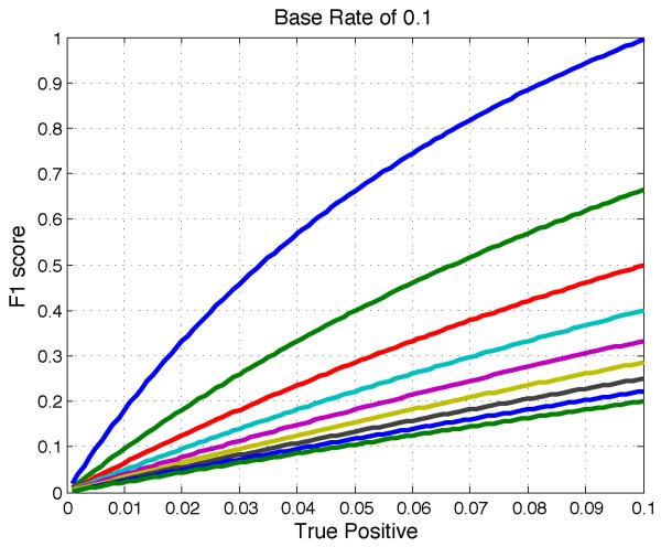
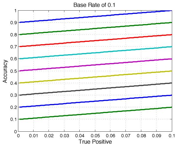
Before explaining optimal thresholding to maximize F1, we first discuss some properties of F1. For any fixed number of actual positives in the gold standard, only two of the four entries in the confusion matrix (Figure 1) vary independently. This is because the number of actual positives is equal to the sum tp + fn while the number of actual negatives is equal to the sum tn + fp. A second basic property of F1 is that it is nonlinear in its inputs. Specifically, fixing the number fp, F1 is concave as a function of tp (Figure 2). By contrast, accuracy is a linear function of tp and tn (Figure 3).

Fig. 2.

Holding base rate and fp constant, F1 is concave in tp. Each line is a different value of fp.

Fig. 3.

Unlike F1, accuracy offers linearly increasing returns. Each line is a fixed value of fp.

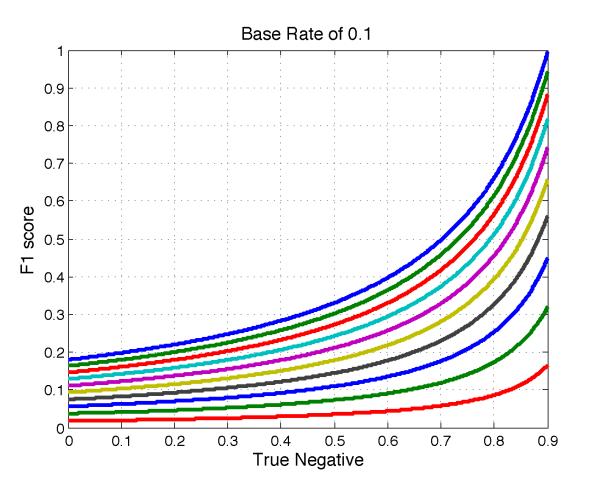
As mentioned in the introduction, F1 is asymmetric. By this, we mean that the score assigned to a prediction P given gold standard G can be arbitrarily different from the score assigned to a complementary prediction P^c given complementary gold standard G^c. This can be seen by comparing Figure 2 with Figure 5. The asymmetry is problematic when both false positives and false negatives are costly. For example, F1 has been used to evaluate the classification of tumors as benign or malignant [1], a domain where both false positives and false negatives have considerable costs.

Fig. 5.

F1 measure for fixed base rate and number fn of false negatives. F1 o ers increasing marginal returns as a function of tn. Each line is a fixed value of fn.

While F1 was developed for single-label information retrieval, as mentioned there are variants of F1 for the multilabel setting. Micro F1 treats all predictions on all labels as one vector and then calculates the F1 measure. Specifically,

$$tp=2\sum _{i=1}^n\sum _{j=1}^m\mathrm{𝟙}(P_{ij}=1)\mathrm{𝟙}(G_{ij}=1).$$

We define fp and fn analogously and calculate the final score using (1). Macro F1, which can also be called per label F1, calculates the F1 for each of the m labels and averages them:

$$F{1}_M(P,G)=\frac{1}{m}\sum _{j=1}^{m}F1(P_{:j},G_{:j}).$$

The per instance F1 measure is similar, but averages F1 over all n examples:

$$F{1}_I(P,G)=\frac{1}{n}\sum _{i=1}^{n}F1(P_{i:},G_{i:}).$$

Accuracy is the fraction of all instances that are predicted correctly:

$$A=\frac{tp+tn}{tp+tn+fp+fn}.$$

Accuracy is adapted to the multilabel setting by summing tp and tn for all labels and then dividing by the total number of predictions:

$$A(P,G)=\frac{1}{nm}\sum _{i=1}^n\sum _{j=1}^m\mathrm{𝟙}(P_{ij}=G_{ij}).$$

The Jaccard index, a monotonically increasing function of F1, is the cardinality of the intersection of the predicted positive set and the actual positive set divided by the cardinality of their union:

$$J=\frac{tp}{tp+fn+fp}.$$

3 Prior Work

Motivated by the widespread use of the F1 measure in information retrieval and in single and multilabel binary classification, researchers have published extensively on its optimization. The paper [8] proposes an outer-inner maximization technique for F1 maximization, while [4] studies extensions to the multilabel setting, showing that simple threshold search strategies are sufficient when individual probabilistic classifiers are independent. Finally, the paper [6] describes how the method of [8] can be extended to efficiently label data points even when classifier outputs are dependent. More recent work in this direction can be found in [19]. However, none of this work directly identifies the relationship of the optimal threshold to the maximum achievable F1 measure over all thresholds, as we do here.

While there has been work on applying general constrained optimization techniques to related measures [13], research often focuses on specific classification methods. In particular, the paper [16] studies F1 optimization for conditional random fields and [14] discusses similar optimization for SVMs. In our work, we study the consequences of maximizing F1 for the general case of any classifier that outputs real-valued scores.

A result similar to a special case below, Corollary 1, was recently derived in [20]. However, the derivation there is complex and does not prove the more general Theorem 1, which describes the optimal decision-making threshold even when the scores output by a classifier are not probabilities.

The batch observation is related to the note in [9] that given a fixed classifier, a specific example may or may not cross the decision threshold, depending on the other examples present in the test data. However, the previous paper does not characterize what this threshold is, nor does it explain the differences between predictions made to optimize micro and macro average F1.

4 Optimal Decision Rule for F1 Maximization

In this section, we provide a characterization of the decision rule that maximizes the F1 measure, and, for a special case, we present a relationship between the optimal threshold and the maximum achievable F1 value.

We assume that the classifier outputs real-valued scores s and that there exist two distributions p(s|t = 1) and p(s|t = 0) that are the conditional probability of seeing the score s when the true label t is 1 or 0, respectively. We assume that these distributions are known in this section; the next section discusses an empirical version of the result. Note also that in this section tp etc. are fractions that sum to one, not counts.

Given p(s|t = 1) and p(s|t = 0), we seek a decision rule D: s → {0, 1} mapping scores to class labels such that the resulting classifier maximizes F1. We start with a lemma that is valid for any D.

Lemma 1. The true positive rate $tp=b{\int }_{s:D\left(s\right)=1}p(s\mid t=1)ds$ where the base rate is b = p(t = 1).

Proof. Clearly $tp={\int }_{s:D\left(s\right)=1}p(t=1\mid s)p\left(s\right)ds$. Bayes rule says that p(t = 1|s) = p(s|t = 1)p(t = 1)/p(s). Hence $tp=b{\int }_{s:D\left(s\right)=1}p(s\mid t=1)ds$.

Using three similar lemmas, the entries of the confusion matrix are

$$\begin{array}{c}\hfill tp=b{\int }_{s:D\left(s\right)=1}p(s\mid t=1)ds\hfill \\ \hfill fn=b{\int }_{s:D\left(s\right)=0}p(s\mid t=1)ds\hfill \\ \hfill fp=(1-b){\int }_{s:D\left(s\right)=1}p(s\mid t=0)ds\hfill \\ \hfill tn=(1-b){\int }_{s:D\left(s\right)=0}p(s\mid t=0)ds.\hfill \end{array}$$

The following theorem describes the optimal decision rule that maximizes F1.

Theorem 1.An example with score s is assigned to the positive class, that is D(s) = 1, by a classifier that maximizes F1 if and only if

$$\frac{b\cdot p(s\mid t=1)}{(1-b)\cdot p(s\mid t=0)}\ge J$$ (2)

where J = tp/(fn + tp + fp) is the Jaccard index of the optimal classifier, with ambiguity given equality in (2).

Before we provide the proof of this theorem, we note the difference between the rule in (2) and conventional cost-sensitive decision making [7] or Neyman-Pearson detection. In both the latter approaches, the right hand side J is replaced by a constant λ that depends only on the costs of 0 – 1 and 1 – 0 classification errors, not on the performance of the classifier on the entire batch. We will later describe how the relationship can lead to undesirable thresholding behavior for applications in the multilabel setting.

Proof. Divide the domain of s into regions of fixed size. Suppose that the decision rule D(·) has been fixed for all regions except a particular region denoted Δ around a point s. Write $P_1\left(\Delta \right)={\int }_{\Delta }p(s\mid t=1)ds$ and define P₀(Δ) similarly.

Suppose that the F1 achieved with decision rule D for all scores besides those in Δ is F1 = 2tp/(2tp + fn + fp). Now, if we add Δ to the positive region of the decision rule, D(Δ) = 1, then the new F1 measure is

$$F{1}^{\prime }=\frac{2tp+2b{P}_1\left(\Delta \right)}{2tp+2b{P}_1\left(\Delta \right)+fn+fp+(1-b)P_0\left(\Delta \right)}.$$

On the other hand, if we add Δ to the negative region of the decision rule, D(Δ) = 0, then the new F1 measure is

$$F{1}^{″}=\frac{2tp}{2tp+fn+b{P}_1\left(\Delta \right)+fp}.$$

We add Δ to the positive region only if F1′ ≥ F1″. With some algebraic simplification, this condition becomes

$$\frac{b{P}_1\left(\Delta \right)}{(1-b)P_0\left(\Delta \right)}\ge \frac{tp}{tp+fn+fp}.$$

Taking the limit |Δ| → 0 gives the claimed result.

If, as a special case, the model outputs calibrated probabilities, that is p(t = 1|s) = s and p(t = 0|s) = 1 - s, then we have the following corollary.

Corollary 1. An instance with predicted probability s is assigned to the positive class by the decision rule that maximizes F1 if and only if s ≥ F/2 where the F1 measure achieved by this optimal decision rule is F = 2tp/(2tp + fn + fp).

Proof. Using the definition of calibration and then Bayes rule, for the optimal decision surface for assigning a score s to the positive class

$$\frac{p(t=1\mid s)}{p(t=0\mid s)}=\frac{s}{1-s}=\frac{p(s\mid t=1)b}{p(s\mid t=0)(1-b)}.$$ (3)

Incorporating (3) in Theorem 1 gives

$$\frac{s}{1-s}\ge \frac{tp}{fn+tp+fp}$$

and simplifying results in

$$s\ge \frac{tp}{2tp+fn+fp}=F∕2.$$

Thus, the optimal threshold in the calibrated case is half the maximum F1 value.

5 Consequences of the Optimal Decision Rule

We demonstrate two consequences of designing classifiers that maximize the F1 measure, which we call the batch observation and the uninformative classifier observation. We will later show with a case study that these can combine to produce surprising and potentially undesirable predictions when macro F1 is optimized in practice.

The batch observation is that a label may or may not be predicted for an instance depending on the distribution of conditional probabilities (or scores) for other instances in the same batch. Earlier, we observed a relationship between the optimal threshold and the maximum achievable F1 value, and demonstrated that this maximum depends on the distribution of conditional probabilities for all instances. Therefore, depending upon the set in which an instance is placed, its conditional probability may or may not exceed the optimal threshold. Note that because an F1 value cannot exceed 1, the optimal threshold cannot exceed 0.5.

Consider for example an instance with conditional probability 0.1. It will be classified as positive if it has the highest probability of all instances in a batch. However, in a different batch, where the probabilities predicted for all other instances are 0.5 and n is large, the maximum achievable F1 measure is close to 2/3. According to the results above, we will then classify this last instance as negative because it has a conditional probability less than 1/3.

An uninformative classifier is one that predicts the same score for all examples. If these scores are calibrated conditional probabilities, then the base rate is predicted for every example.

Theorem 2. Given an uninformative classifier for a label, optimal thresholding to maximize expected F1 results in classifying all examples as positive.

Proof. Given an uninformative classifier, we seek the threshold that maximizes 𝔼(F1). The only choice is how many labels to predict. By symmetry between the instances, it does not matter which instances are labeled positive.

Let a = tp + fn be the number of actual positives and let c = tp + fp be a fixed number of positive predictions. The denominator of the expression for F1 in Equation (1), that is 2tp + fp + fn = a + c, is then constant. The number of true positives, however, is a random variable. Its expected value is equal to the sum of the probabilities that each example predicted positive actually is positive:

$$𝔼\left(F1\right)=\frac{2{\Sigma }_{i=1}^{c}b}{a+c}=\frac{2c\cdot b}{a+c}$$

where b = a/n is the base rate. To maximize this expectation as a function of c, we calculate the partial derivative with respect to c, applying the product rule:

$$\frac{\partial }{\partial c}𝔼\left(F1\right)=\frac{\partial }{\partial c}\frac{2c\cdot b}{a+c}=\frac{2b}{a+c}-\frac{2c\cdot b}{{(a+c)}^2}.$$

Both terms in the difference are always positive, so we can show that the derivative is always positive by showing that

$$\frac{2b}{a+c}>\frac{2c\cdot b}{{(a+c)}^2}.$$

Simplification gives the condition 1 < c/(a + c). As this condition always holds, the derivative is always positive. Therefore, whenever the frequency of actual positives in the test set is nonzero, and the predictive model is uninformative, then expected F1 is maximized by predicting that all examples are positive.

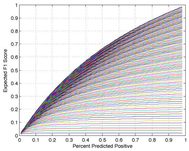
Figure 6 shows that for small base rates, an optimally thresholded uninformative classifier achieves 𝔼(F1) close to 0, while for high base rates 𝔼(F1) is close to 1. We revisit this point in the next section in the context of maximizing macro F1.

Fig. 6.

The expected F1 measure of an optimally thresholded random guess is highly dependent on the base rate.

6 Multilabel Setting

Different measures are used to measure different aspects of a system’s performance. However, changing the measure that is optimized can change the optimal predictions. We relate the batch observation to discrepancies between predictions that are optimal for micro versus macro averaged F1. We show that while performance on rare labels is unimportant for micro F1, macro F1 is dominated by performance on these labels. Additionally, we show that macro averaging F1 can conceal the occurrence of uninformative classifier thresholding.

Consider the equation for micro averaged F1, for m labels with base rates b_i. Suppose that tp, fp, and fn are fixed for the first m − 1 labels, and suppose that b_m is small compared to the other b_i. Consider (i) a perfect classifier for label m, (ii) a trivial classifier that never predicts label m, and (iii) a trivial classifier that predicts label m for every example. The perfect classifier increases tp by a small amount b_m · n, the number of actual positives for the rare label m, while contributing nothing to the counts fp and fn:

$$F{1}^{\prime }=\frac{2(tp+b_m\cdot n)}{2(tp+b_m\cdot n)+fp+fn}.$$

The trivial classifier that never predicts label m increases fn by the same small amount:

$$F{1}^{″}=\frac{2tp}{2tp+fp+(fn+b_m\cdot n)}.$$

Finally, the trivial classifier that predicts label m for every example increases fp by a large amount n(1-b_m). Clearly this last classifier leads to micro average F1 that is much worse than that of the perfect classifier for label m. However, F 1′ and F 1″ both tend to the same value, namely 2tp/(2tp + fp + fn), as b_m tends to zero. Hence, for a label with very small base rate, a perfect classifier does not improve micro F1 noticeably compared to a trivial all-negative classifier. It is fair to say that performance on rare labels is unimportant for micro F1.

Now consider the context of macro F1, where separately calculated F1 measures over all labels are averaged. Consider the two label case where one label has a base rate of 0.5 and the other has a base rate of 0.1. The corresponding F1 measures for trivial all-positive classifiers are 0.67 and 0.18 respectively. Thus the macro F1 for trivial classifiers is 0.42. An improvement to perfect predictions on the rare label increases macro F1 to 0.83, while the same improvement on the common label only increases macro F1 of 0.59. Hence it is fair to say that macro F1 emphasizes performance on rare labels, even though it weights performance on every label equally.

For a rare label with an uninformative predictive model, micro F1 is optimized by classifying all examples as negative, while macro F1 is optimized by classifying all examples as positive. Optimizing micro F1 as compared to macro F1 can be thought of as choosing optimal thresholds given very different batches. If the base rates and distributions of conditional probabilities predicted for instances vary from label to label, so will the optimal binary predictions. Generally, labels with small base rates and less informative classifiers will be over-predicted when maximizing macro F1, and under-predicted when maximizing micro F1. We present empirical evidence of this phenomenon in the following case study.

7 Case Study

This section discusses a case study that demonstrates how in practice, thresholding to maximize macro F1 can produce undesirable predictions. To our knowledge, a similar real-world case of pathological behavior has not been previously described in the literature, even though macro averaging F1 is a common approach.

We consider the task of assigning tags from a controlled vocabulary of 26,853 MeSH terms to articles in the biomedical literature based on their titles and abstracts. We represent each abstract as a sparse bag-of-words vector over a vocabulary of 188,923 words. The training data consists of a matrix A with n rows and d columns, where n is the number of abstracts and d is the number of features in the bag of words representation. We apply a tf-idf text preprocessing step to the bag of words representation to account for word burstiness [10] and to elevate the impact of rare words.

Because linear regression models can be trained for multiple labels efficiently, we choose linear regression as a predictive model. Note that square loss is a proper loss function and yields calibrated probabilistic predictions [12]. Further, to increase the speed of training and prevent overfitting, we approximate the training matrix A by a rank restricted A_k using singular value decomposition. One potential consequence of this rank restriction is that the signal of extremely rare words can be lost. This can be problematic when rare terms are the only features of predictive value for a label.

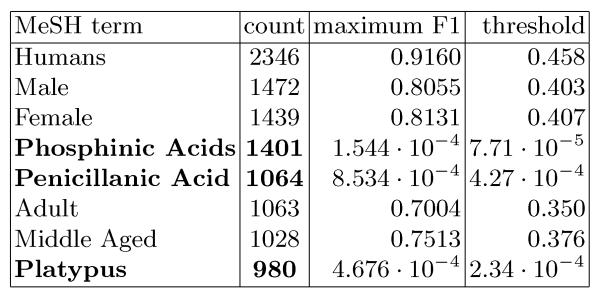
Given the probabilistic output of each classifier and the results relating optimal thresholds to maximum attainable F1, we designed three different plug-in rules to maximize micro, macro and per instance average F1. Inspection of the predictions to maximize micro F1 revealed no irregularities. However, inspecting the predictions thresholded to maximize performance on macro F1 showed that several terms with very low base rates were predicted for more than a third of all test documents. Among these terms were “Platypus”, “Penicillanic Acids” and “Phosphinic Acids” (Figure 7).

Fig. 7.

Selected frequently predicted MeSH terms. Columns show the term, the number of times it is predicted for a given test set, the empirical maximum achieved F1 measure, and the empirical threshold that achieves this maximum. When F1 is optimized separately for each term, low thresholds are chosen for rare labels (bold) with uninformative classifiers.

In multilabel classification, a label can have low base rate and an uninformative classifier. In this case, optimal thresholding requires the system to predict all examples positive for this label. In the single-label case, such a system would achieve a low F1 and not be used. But in the macro averaging multilabel case, the extreme thresholding behavior can take place on a subset of labels, while the system manages to perform well overall.

8 A Winner’s Curse

In practice, decision rules that maximize F1 are often set empirically, rather than analytically. That is, given a set of validation examples with predicted scores and true labels, rules for mapping scores to labels are selected that maximize F1 on the validation set. In such situations, the optimal threshold can be subject to a winner’s curse [2] where a sub-optimal threshold is chosen because of sampling effects or limited training data. As a result, the future performance of a classifier using this threshold is worse than the anticipated performance. We show that threshold optimization for F1 is particularly susceptible to this phenomenon.

In particular, different thresholds have different rates of convergence of empirical F1 with number of samples n. As a result, for a given n, comparing the empirical performance of low and high thresholds can result in suboptimal performance. This is because, for a fixed number of samples, some thresholds converge to their true error rates fast, while others have higher variance and may be set erroneously. We demonstrate these ideas for a scenario with an uninformative model, though they hold more generally.

Consider an uninformative model, for a label with base rate b. The model is uninformative in the sense that output scores are s_i = b + n_i for examples i, where $n_i=\mathcal{N}(0,{\sigma }^2)$. Thus, scores are uncorrelated with and independent of the true labels. The empirical accuracy for a threshold t is

$$A\left(t\right)=\frac{1}{n}\sum _{i\in +}1[s_i\ge t]+\frac{1}{n}\sum _{i\in -}1[s_i\le t]$$ (4)

where + and − index the positive and negative class respectively. Each term in Equation (4) is the sum of O(n) i.i.d random variables and has exponential (in n) rate of convergence to the mean irrespective of the base rate b and the threshold t. Thus, for a fixed number T of threshold choices, the probability of choosing the wrong threshold is less than T2^−εn where ε depends on the distance between the optimal and next nearest threshold. Even if errors occur, the most likely errors are thresholds close to the true optimal threshold, a consequence of Sanov’s theorem [3].

Consider how to select an F1-maximizing threshold empirically, given a validation set of ground truth labels and scores from an uninformative classifier. The scores s_i can be sorted in decreasing order (w.l.o.g.) since they are independent of the true labels for an uninformative classifier. Based on the sorted scores, we empirically select the threshold that maximizes the F1 measure F on the validation set. The optimal empirical threshold will lie between two scores that include the value F/2, when the scores are calibrated, in accordance with Theorem 1.

The threshold s that classifies all examples positive (and maximizes F1 analytically by Theorem 2) has an empirical F1 value close to its expectation of $\frac{2b}{1+b}=\frac{2}{1+1∕b}$ since tp, fp and fn are all estimated from the entire data. Consider a threshold s that classifies only the first example positive and all others negative. With probability b, this threshold has F1 value 2/(2 + b·n), which is worse than that of the optimal threshold only when

$$b\ge \frac{\sqrt{1+8∕n}-1}{2}.$$

Despite the threshold s being far from optimal, it has a constant probability of having a better F1 value on validation data, a probability that does not decrease with n, for n < (1 - b)/b². Therefore, optimizing F1 has a sharp threshold behavior, where for n < (1 - b)/b² the algorithm incorrectly selects large thresholds with constant probability, whereas for larger n it correctly selects small thresholds. Note that identifying optimal thresholds for F1 is still problematic since it then leads to issues identified in the previous section. While these issues are distinct, they both arise from the nonlinearity of the F1 measure and its asymmetric treatment of positive and negative labels.

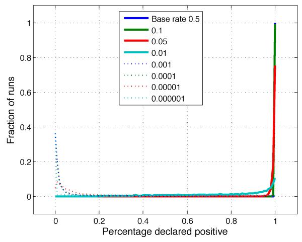
Figure 8 shows the result of simulating this phenomenon, executing 10,000 runs for each setting of the base rate, with n = 10⁶ samples for each run used to set the threshold. Scores are chosen using variance σ² = 1. True labels are assigned at the base rate, independent of the scores. The threshold that maximizes F1 on the validation set is selected. We plot a histogram of the fraction predicted positive as a function of the empirically chosen threshold. There is a shift from predicting almost all positives to almost all negatives as the base rate is decreased. In particular, for low base rate, even with a large number of samples, a small fraction of examples are predicted positive. The analytically derived optimal decision in all cases is to predict all positive, i.e. to use a threshold of 0.

Fig. 8.

The distribution of experimentally chosen thresholds changes with varying base rate b. For small b, a small fraction of examples are predicted positive even though the optimal thresholding is to predict all positive.

9 Discussion

In this paper, we present theoretical and empirical results describing properties of the F1 performance measure for binary and multilabel classification. We relate the best achievable F1 measure to the optimal decision-making threshold and show that when a classifier is uninformative, classifying all instances as positive maximizes F1. In the multilabel setting, this behavior is problematic when the measure to maximize is macro F1 and for some labels their predictive model is uninformative. In contrast, we demonstrate that given the same scenario, micro F1 is maximized by predicting those labels for all examples to be negative. This knowledge can be useful as such scenarios are likely to occur in settings with a large number of labels. We also demonstrate that micro F1 has the potentially undesirable property of washing out performance on rare labels.

No single performance measure can capture every desirable property. For example, for a single binary label, separately reporting precision and recall is more informative than reporting F1 alone. Sometimes, however, it is practically necessary to define a single performance measure to optimize. Evaluating competing systems and objectively choosing a winner presents such a scenario. In these cases, it is important to understand that a change of performance measure can have the consequence of dramatically altering optimal thresholding behavior.

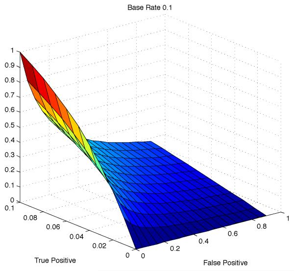
Fig. 4.

Given a fixed base rate, the F1 measure is a nonlinear function with two degrees of freedom.

References

- 1.Akay MF. Support vector machines combined with feature selection for breast cancer diagnosis. Expert Systems with Applications. 2009;36(2):3240–3247. [Google Scholar]
- 2.Capen EC, Clapp RV, Campbell WM. Competitive bidding in high-risk situations. Journal of Petroleum Technology. 1971;23(6):641–653. [Google Scholar]
- 3.Cover TM, Thomas JA. Elements of information theory. John Wiley & Sons; 2012. [Google Scholar]
- 4.del Coz JJ, Diez J, Bahamonde A. Learning nondeterministic classifiers. Journal of Machine Learning Research. 2009;10:2273–2293. [Google Scholar]
- 5.Dembczynski K, Kotłowski W, Jachnik A, Waegeman W, Hüllermeier E. Optimizing the F-measure in multi-label classification: Plug-in rule approach versus structured loss minimization. ICML; 2013. [Google Scholar]
- 6.Dembczyński K, Waegeman W, Cheng W, Hüllermeier E. An exact algorithm for F-measure maximization. Neural Information Processing Systems; 2011. [Google Scholar]
- 7.Elkan C. The foundations of cost-sensitive learning; International joint conference on artificial intelligence; 2001.pp. 973–978. [Google Scholar]
- 8.Jansche M. A maximum expected utility framework for binary sequence labeling; Annual Meeting of the Association For Computational Linguistics; 2007.p. 736. [Google Scholar]
- 9.Lewis DD, ACM Evaluating and optimizing autonomous text classification systems; Proceedings of the 18th annual international ACM SIGIR conference on research and development in information retrieval; 1995.pp. 246–254. [Google Scholar]
- 10.Madsen R, Kauchak D, Elkan C. Modeling word burstiness using the Dirichlet distribution; Proceedings of the International Conference on Machine Learning (ICML); Aug 2005.pp. 545–552. [Google Scholar]
- 11.Manning C, Raghavan P, Schütze H. Introduction to information retrieval. Vol. 1. Cambridge University Press; 2008. [Google Scholar]
- 12.Menon A, Jiang X, Vembu S, Elkan C, Ohno-Machado L. Predicting accurate probabilities with a ranking loss; Proceedings of the International Conference on Machine Learning (ICML); Jun 2012; [PMC free article] [PubMed] [Google Scholar]
- 13.Mozer MC, Dodier RH, Colagrosso MD, Guerra-Salcedo C, Wolniewicz RH. Prodding the ROC curve: Constrained optimization of classifier performance. NIPS; 2001. pp. 1409–1415. [Google Scholar]
- 14.Musicant DR, Kumar V, Ozgur A, et al. Optimizing F-measure with support vector machines; FLAIRS Conference; 2003.pp. 356–360. [Google Scholar]
- 15.Sokolova M, Lapalme G. A systematic analysis of performance measures for classification tasks. Information Processing and Management. 2009;45:427–437. [Google Scholar]
- 16.Suzuki J, McDermott E, Isozaki H, Association for Computational Linguistics Training conditional random fields with multivariate evaluation measures; Proceedings of the 21st International Conference on Computational Linguistics and the 44th annual meeting of the Association for Computational Linguistics; 2006.pp. 217–224. [Google Scholar]
- 17.Tan S. Neighbor-weighted k-nearest neighbor for unbalanced text corpus. Expert Systems with Applications. 2005;28:667–671. [Google Scholar]
- 18.Tsoumakas Grigorios, Katakis I. Multi-label classification: An overview. International Journal of Data Warehousing and Mining. 2007;3(3):1–13. [Google Scholar]
- 19.Ye N, Chai KM, Lee WS, Chieu HL. Optimizing F-measures: A tale of two approaches; Proceedings of the International Conference on Machine Learning; 2012. [Google Scholar]
- 20.Zhao MJ, Edakunni N, Pocock A, Brown G. Beyond Fano’s inequality: Bounds on the optimal F-score, BER, and cost-sensitive risk and their implications. Journal of Machine Learning Research. 2013;14(1):1033–1090. [Google Scholar]