The Mesosphere and Metals: Chemistry and Changes

1. Introduction

The subject of this review is the atmospheric chemistry of the metals which ablate from meteoroids in the Earth’s upper atmosphere. The major meteoric species are Fe, Mg, Si, and Na, against which two minor species, Ca and K, offer surprising contrasts. These metals exist as layers of atoms between about 80 and 105 km and atomic ions at higher altitudes. Below 85 km they form compounds—oxides, hydroxides, and carbonates—which polymerize into nanometer-sized meteoric smoke particles (MSPs). These particles probably act as condensation nuclei for clouds in the mesosphere and stratosphere and eventually after about 4 years are deposited at the Earth’s surface. The subject of meteoric metal chemistry was reviewed in 1991¹ and 2003,² and there were also more focused reviews on laboratory studies of metal reactions in 1994³ and 2002⁴ and the atmospheric modeling of metals in 2002.⁵

The present review will therefore concentrate on the many developments that have taken place in the past decade. On the observational side, these developments include the near-global measurement of the Na, K, Mg, and Mg⁺ layers from satellite-borne spectrometers and lidar observations of Na and Fe from several Antarctic observatories, the discovery that metal atoms are removed in the vicinity of noctilucent (or polar mesospheric) clouds, the surprising observation of metal atoms up to around 180 km in the thermosphere, the unexpected finding that the ratio of the Na d lines in the terrestrial nightglow is variable, the first observations of the molecular bands of FeO and NiO in the nightglow, the first measurements of the vertical flux of Na atoms in the upper mesosphere, the measurement of MSPs from rockets, incoherent scatter radars, satellites, and aircraft, and measurements of the depositional flux of meteoric smoke in polar ice cores.

Laboratory measurements (including the application of quantum chemistry calculations) have addressed several issues: the ion and neutral gas-phase chemistries of compounds containing Fe, Ca, Mg, Si, and K, leading to the first chemically closed reaction schemes for these metals, the uptake of metal atoms on low-temperature ice surfaces and the resulting photoelectric emission, understanding the variable Na d line ratio observations, and the formation of a variety of iron oxide and Fe–Mg–silicate nanoparticles as analogues of meteoric smoke.

There have also been significant developments in modeling: a chemical ablation model to predict the evaporation rates of individual elements from a meteoroid, coupling this ablation model with an astronomical model of dust input to generate the meteoric input function (MIF), the inclusion of the MIF together with metal chemistry in a whole atmosphere chemistry climate model to create the first global models of the Na, Fe, Mg, and K layers, an explanation for the 50 year old puzzle of why the Na and K layers exhibit such different seasonal behavior, modeling the growth and transport of MSPs through the mesosphere and stratosphere, the paleoclimate implications of an enhanced cosmic dust input, and the climate implications of the deposition of meteoric Fe into the Southern Ocean.

The present review is divided into five sections following this Introduction. Section 2 is a general review of the mesosphere and lower thermosphere from the perspective of understanding the metal layers and the sensitivity of this atmospheric region to solar activity and longer term anthropogenic changes. Section 3 describes the atmospheric chemistry of the meteoric metals and then reviews observations of the metal layers and MSPs. Section 4 deals with laboratory and theoretical studies of gas-phase metal reactions and particle formation under mesospheric conditions. Section 5 is concerned with the development of global models of metal chemistry which describe the input and ablation of cosmic dust, the gas-phase chemistry of metallic species, the formation of MSPs, and transport to the Earth’s surface. Section 6 is then a summary with a discussion of future directions for the field.

2. The Mesosphere and Lower Thermosphere

2.1. Physical Characteristics

The mesosphere begins at the stratopause (∼50 km), which is characterized by a local temperature maximum caused by stratospheric ozone absorbing solar UV radiation above 200 nm. Figure 1 shows the temperature of the atmosphere in January and July as a function of height (50–110 km) and latitude. The data are an average of 8 years of output (2004–2011) from the Whole Atmosphere Community Climate Model (WACCM).⁶ Figure 1 shows that the temperature decreases with height through the mesosphere up to the mesopause, which occurs around 85 km in summer and 100 km in winter. The thermosphere begins above the mesopause. The absorption of extreme UV radiation at wavelengths below 180 nm, mostly by O₂, leads to a rapid warming with altitude. Kinetic temperatures in the thermosphere reach 400–1000 K (and sometimes even higher during solar storms). Because the pressure is very low (<10^–7 bar above 110 km), the vibrational and rotational modes of molecules are not usually in local thermodynamic equilibrium.⁷

Figure 1.

Temperature (K) as a function of latitude and height in the MLT for January (left panel) and July (right panel) (averaged from 2004 to 2011). Also plotted are wind vectors (m s^–1) which combine the meridional wind v with the vertical wind w (×500). Output from the Whole Atmosphere Community Climate Model.

The region extending from about 70 to 110 km is usually referred to as the mesosphere/lower thermosphere (MLT) region. The turbopause, which is a useful definition of the boundary between the atmosphere and space, occurs at around 105 km and thus falls within the MLT. At this boundary the pressure falls to less than 5 × 10^–7 bar and the mean free path of air molecules approaches 1 m, at which point bulk turbulent motion starts to break down and molecular diffusion dominates. The separation of molecules by mass is then able to occur through gravitational settling of the heavier species (CO₂ and Ar in the lower thermosphere) relative to the lighter components; only H, H₂, and He occur at significant concentrations above 500 km.⁷

Figure 2 shows schematically the energy balance in the MLT. The MLT is subject to high-energy inputs from above in the form of solar electromagnetic radiation and energetic particles (mostly electrons and protons of solar origin) which precipitate downward from the magnetosphere. The resulting photodissociation, photoionization, and high-energy collisions generate radicals and ions, often with internal excitation. The most important of these processes is the photodissociation of O₂ via absorption in the Schumann–Runge continuum (130–175 nm) and the Schumann–Runge bands (175–195 nm), with a less important contribution from O₃ photolysis.⁸ The resulting O atoms participate in a number of highly exothermic reactions (see section 2.2), which convert chemical potential energy into kinetic energy. A similar amount of molecular kinetic energy is deposited from below by the breaking of gravity waves. Finally, the dominant cooling process is via emission at 15 μm from CO₂ (the degenerate bending mode), which is efficiently excited by collision with O atoms.⁹ Note that infrared heating from below is unimportant because the atmospheric pressure is too low for efficient vibrational-to-translational energy transfer. Although it is not clear that the mesosphere is in global mean radiative balance on monthly or seasonal time scales, the following relation probably holds:⁸

E1

where the terms on the left-hand side represent the integrated energy inputs from O₂ photodissociation, O₃ photodissociation, gas-phase reaction exothermicity, and breaking gravity waves, respectively , and the right-hand side is the integrated infrared emission from CO₂.

Figure 2.

Energy balance in the MLT: roughly equal inputs of energy from absorption of solar energy by O₂ and O₃ and breaking gravity waves are balanced by radiative loss principally through 15 μm emission of CO₂.

The low temperatures in the mesosphere (Figure 1) are caused by limited local heating on the left-hand side of eq E1. This is because most solar EUV is removed by O₂ absorption in the thermosphere. Furthermore, the pressure range in the mesosphere (10^–6–10^–3 bar) is too low for O₃ to form efficiently through the recombination of O and O₂ (in contrast to the stratosphere). The high concentration of O atoms above 80 km (see below) means that radiative cooling from CO₂ on the right-hand side of eq E1 is very efficient.

Figure 1 also shows that, unlike the lower atmosphere, which is warmer in summer, the coldest part of the MLT region is actually the summer polar mesopause around 85 km. The explanation for this counterintuitive observation appears to be the effect of gravity waves, which originate in the troposphere from a variety of sources including orographic forcing, wind shears, cumulonimbus cloud formation, and cyclonic fronts.⁷ Much of the energy and momentum flux of these waves is filtered out in the stratosphere, but a significant portion of the shorter period waves propagate to the upper mesosphere. As a wave travels upward through the mesosphere, the wave amplitude increases with falling pressure until the wave becomes unstable and breaks, depositing both energy and momentum in the MLT. This exerts a drag on the zonal wind, resulting in a meridional flow in the middle and upper mesosphere toward the winter pole. The wind vectors in Figure 1 show the combined meridional wind (v) and vertical wind (w, multiplied here by a factor of 500 for purposes of visualization). The upwelling air in the summer high latitudes, which feeds this meridional flow, is cooled by adiabatic expansion, leading to very low temperatures which can fall below 120 K (note that if the summer mesopause at high latitudes were in thermal equilibrium, it would have a temperature around 220 K). A striking feature of this meridional circulation is that air from the entire global mesosphere is then funneled down into the lower stratosphere within the winter polar vortex, particularly over the Antarctic during June to August (Figure 1, right-hand panel). As discussed in sections 5.3 and 5.4, this so-called residual circulation transports MSPs from the mesosphere to the lower stratosphere, before entrainment into the troposphere and finally deposition at the surface.

Figure 3 illustrates the temperature at 87 km as a function of latitude and month. This height is useful for understanding the behavior of the meteoric metal layers, as it lies about 2 km above the peak of the Fe layer and about 2 km below the peaks of the Na, K, Ca, and Mg layers.² Note that there is very little seasonal variation between about 30° S and 30° N; in contrast, at high latitudes the absolute temperature can increase by a factor of ∼1.5 from summer to winter.

Figure 3.

Zonally averaged temperature (K) at 87 km as a function of latitude and month. Output from the Whole Atmosphere Community Climate Model.

2.2. Dominant Chemistry

Atomic oxygen drives nearly all the chemistry in the MLT: it controls the concentrations of radicals such as H, OH, and HO₂ and is ultimately responsible for the presence of the metal atom layers which are a focus of this review (sections 3.1 and 3.2), it participates either directly or indirectly in all the reactions that contribute to airglow emission layers between 83 and 100 km (section 3.2), it governs the chemical lifetime of metallic ions in sporadic E layers (section 3.2), it controls the charging of MSPs below 90 km (section 3.3), and it is central to the radiative balance of the MLT, through both chemical heating reactions and radiative cooling with CO₂ (section 2.1).

Figure 4a shows the diurnal variation of atomic O as a function of height at a midlatitude location in the northern hemisphere. What is immediately striking is that whereas there is a pronounced diurnal variation below 80 km, with the O essentially disappearing at night, above 84 km there is almost no diurnal variation. This sudden change around 82 km, referred to as the O atom ledge (or shelf), is illustrated even more clearly in Figure 5, which shows measured atomic O profiles made by rocket-borne resonance fluorescence instruments (employing the O(2³S₁–2³P₂) transition at 130.2 nm).¹⁰ These profiles were measured between 1978 and 1993 from rockets launched during summer in the Arctic under conditions of twilight (see ref (10) for further details). In the sunlit upper mesosphere, the O concentration below the ledge is still measurable despite a 3 orders of magnitude decrease. Note both the variability of the profiles and the very sharp transition at the base of the O atom ledge around 82–84 km, which is well described by a 1-D model (the dashed line in Figure 5).¹⁰

Figure 4.

Diurnal variation as a function of the height of the (a) O density (10¹⁰ atom cm^–3), (b) H density (10⁷ atom cm^–3), and (c) O₃ density (10⁹ molecules cm^–3) for October at Kühlungsborn, Germany (54° N, 12° E) (averaged from 2004 to 2011). Output from the Whole Atmosphere Community Climate Model.

Figure 5.

Atomic O measurements made by rocket-borne resonance fluorescence instruments during summer in Northern Sweden (67.9° N). Adapted with permission from ref (10). Copyright 2005 Copernicus Publications on behalf of the European Geosciences Union.

The rate-determining step in removal of atomic O is the recombination reaction R1 to form O₃. The rate of this reaction at its low-pressure limit is pressure dependent and hence varies as [O₂]². Since the atmospheric scale height is only about 4 km in the cold MLT, the rate of reaction R1 decreases by an order of magnitude for every 5 km increase in height. Above 82 km the time constant for O removal exceeds 12 h, so that there is almost no diurnal variation. O is removed principally by the sequence of reactions R1–R5:

R1

R2

R3

R4

R5

Note that the sequences R1–R2–R3 and R4–R5–R3 are catalytic cycles which effectively recombine O atoms (the direction reaction O + O (+M) → O₂ is very slow). The catalyst, atomic H, is produced from the photolysis of H₂O (see below). Figure 4b shows that the diurnal profile of H is very similar to that of O, also with a shelf around 82 km. This is a result of the close coupling of these species through reactions R2 –R5. In contrast, O₃ displays the opposite behavior (Figure 4c), with little diurnal variability below 75 km and a pronounced diurnal variation above 80 km; there is a 10-fold increase at night when photolysis ceases.

Figure 6 illustrates the seasonal variability of diurnally averaged NO, H₂O, and H as a function of height. Figure 6a shows that there is a substantial source of NO in the lower thermosphere above 90 km, mainly from reaction R6 involving electronically excited N(²D) atoms which are produced from highly exothermic ion–molecule reactions such as R7:

R6

R7

where N₂⁺ is produced by photoionization or energetic particle bombardment of N₂. This chemistry results in a substantial flux of NO into the mesosphere during the winter months at high latitudes because of descent in the polar vortex (Figure 1), whereas in summer the NO density in the middle mesosphere is lowest (Figure 6a). Figure 6b shows that the H₂O density falls by only a factor of 20 between 50 and 75 km, whereas the total atmospheric density decreases by a factor of about 60. This increasing mixing ratio (or mole fraction) of H₂O with height is caused by production of H₂O in the lower mesosphere from the oxidation of CH₄ propagating up from the stratosphere. However, above 80 km the mixing ratio of H₂O decreases rapidly due to photolysis by solar Lyman-α radiation at 121.6 nm, which is able to penetrate down to ∼80 km because the absorption cross-section of O₂ in the Schumann–Runge continuum happens to be very small just around the Lyman-α wavelength.⁷ Note that during the summer months (May to September in Figure 6b) there is a roughly 3-fold increase in H₂O in the MLT due to the residual circulation (Figure 1). This is mirrored by a similar increase in atomic H, which reaches a maximum around 85 km during summer (Figure 6c).

Figure 6.

Seasonal variation as a function of the height of the zonally averaged (a) NO density (10⁸ molecules cm^–3), (b) H₂O density (10⁷ molecules cm^–3), and (c) H density (10⁷ atom cm^–3) at 54° N (averaged from 2004 to 2011). Output from the Whole Atmosphere Community Climate Model.

Another important aspect of the MLT is that significant concentrations of positive ions, negative ions and electrons occur above 70 km. The primary source of ions and electrons in the lower E region above 100 km is solar X-ray and extreme ultraviolet radiation at wavelengths below 103 nm. Important components of this are the Lyman-β (102.6 nm) line, the C III line (97.7 nm), the He I and II lines at 58.4 and 30.4 nm, and soft X-rays at λ < 1 nm. The photoionization of NO by Lyman-α radiation is the main source of plasma in the mesosphere below 90 km. The electron density profile is divided into three regions: in the D region (70–95 km), proton hydrates (i.e., H⁺(H₂O)_n, n ≥ 1), negative ions, and negatively charged MSPs (section 3.3) dominate; in the E region (95–170 km), O₂⁺ and NO⁺ are the dominant ions, balanced by free electrons; and above this in the F region (170–500 km), O⁺ and N⁺ ions dominate. The general ion chemistry of the E and F regions, including metallic ion chemistry, has been reviewed recently by Pavlov.¹¹

2.3. Sensitivity to Change

There has been increasing interest in the response of the mesosphere and thermosphere to anthropogenic climate change ever since the modeling prediction by Roble and Dickinson¹² that the global average mesospheric temperature would cool by approximately 10 K for a doubled CO₂ scenario. Modeling studies have identified the main drivers of the observed trends, most notably the increase of greenhouse gases which act as radiative coolers at these altitudes in contrast to their radiative warming properties below 20 km.^13,14 Other drivers include stratospheric O₃ depletion,¹³ changes in atmospheric dynamics,¹⁵ changes in solar and geomagnetic activity,¹⁶ and changes in the Earth’s magnetic field.¹⁷ A number of comprehensive reviews on these trends were published between 2005 and 2012.¹⁸⁻²¹ Here we present a summary of the current state of trend studies.

2.3.1. Trends in Temperature and Dynamics

Temperature is the predominant atmospheric parameter which is perturbed by changes in greenhouse gas concentrations.²² It is worth noting that the temperature change in the mesosphere over the past two decades is similar to the diurnal temperature variation, which makes the trend easier to detect than in the troposphere, where the diurnal variation is much larger than the warming over the past 150 years. Cooling trends in the mesosphere are apparent in long-term records from ground-based, rocketsonde, and satellite data.²³⁻³³ A schematic overview of the observed temperature trends in the neutral and ionized atmosphere is provided in Figure 7. Laštovička et al.¹⁹ have provided a comprehensive summary of these trends: a cooling trend of 1–3 K decade^–1 within the lower and middle mesosphere (50–70 km) and 0–10 K decade^–1 within the upper mesosphere (70–80 km). The larger range in estimates for the upper mesosphere arises principally from the cooling rates derived from rocketsonde data, which have significant associated uncertainties. In the mesopause region (80 and 100 km), many observations^26,34−37 and modeling studies^14,38 indicate near-zero temperature trends, although some recent studies³⁹⁻⁴¹ have reported cooling trends of up to 3 K decade^–1.

Figure 7.

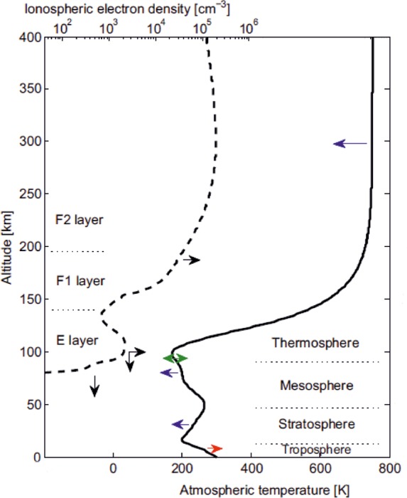
Structure and trends in the Earth’s atmosphere. The atmospheric layers on the right are defined by the temperature profile (solid line, bottom abscissa). The ionospheric layers on the left are defined by the electron density profile (broken line, top abscissa). Arrows denote the direction of observed changes in the past 3–4 decades: red, warming; blue, cooling; green, no overall temperature change; black, changes in the maximum electron density (horizontal) and the height of ionospheric layers (vertical). Adapted with permission from ref (22). Copyright 2006 American Association for the Advancement of Science.

As discussed in section 2.1, the MLT is sensitive to perturbations from both below (upward propagating atmospheric waves and dynamical forcing) and above (solar radiation and energetic particle precipitation). Various workers^{21,36,39,40,42} have noted significant seasonal and monthly variability within the data records, which makes the derived trend very reliant on the choice and length of the analysis period. An example of this is illustrated in Figure 8 from a recent review²¹ which compares temperature trends in the tropics as a function of altitude from several different data sets: U.S. rocketsonde data from 1969 to 1990,⁴³ Indian rocketsonde data from 1971 to 2012,⁴⁴ Brazilian lidar data from 1993 to 2006,⁴⁵ Indian lidar data from 1998 to 2009,⁴⁶ and HALOE satellite data from 1991 to 2005.⁴⁰ Inspection of Figure 8 shows that although the data sets qualitatively agree—displaying cooling trends at all altitudes—they differ markedly in the strength of these trends. This was attributed predominantly to changes in stratospheric O₃ over the total period covered by these different data sets (1969–2009). The weakest cooling trend is shown by the HALOE observations which are post-1991 when the net O₃ effect was close to zero.⁴⁰

Figure 8.

Annual mean long-term temperature trends (K decade^–1) in the mesosphere over the tropical latitudes. The rocketsonde trends of the 1970s and 1980s are compared with the trend obtained during the past two decades using satellite and lidar data (see the text for further details). The horizontal line shading represents roughly the range of trends as revealed during the past two decades. Reprinted with permission from ref (21). Copyright 2011 John Wiley & Sons, Inc.

Changes in stratospheric O₃ have an important influence on the constituents and dynamics in the mesosphere^{13,19,47−51} and appear to be responsible for the observed nonlinearity in trends of a variety of parameters.^{13,19,40,48,50,52−54} While CO₂ is the main driver and accounts for a largely monotonic linear background in these trends, a modeling study by Lübken et al.⁵⁰ indicates that O₃ contributes approximately one-third to the decadal variations. Ozone depletion prior to the mid-1990s resulted in a strong cooling trend. Since then, a recovery in O₃ concentration has been observed.⁵⁵⁻⁵⁷

A potentially significant impact of middle and upper atmospheric cooling would be changes in the mean circulation caused by long-term changes in gravity wave activity, planetary waves, and tides.^21,54 However, these trends are likely to be regionally and seasonally variable and hence difficult to detect.^15,54,58,59 Some studies⁵⁸ suggest that there is no apparent trend in gravity wave activity in the MLT, while others^15,60 point to a weak positive trend. There has been no clear pattern in trends of planetary wave activity^19,61 and some controversy in the sign and magnitude of trends in tidal activity.^59,62 There is also no consistent trend in the zonal and meridional winds in the mesosphere.^54,62,63

2.3.2. Polar Mesospheric Clouds and Other Layered Phenomena

Polar mesospheric clouds (PMCs) have received a great deal of attention as sensitive indicators of climate change due to their dependence on temperature and water vapor.^64,65 The clouds were first reported during June 1885 over middle and northern Europe. When viewed from the ground, they have historically been referred to as noctilucent clouds (NLCs). The clouds form at the very cold temperatures (<145 K) are found within the summer mesopause region at high latitudes (Figure 1), at altitudes between 82 and 85 km.⁶⁶ Thomas et al.⁶⁷ proposed that the increased release of CH₄ at the Earth’s surface, and its oxidation by O(¹D) and OH in the stratosphere, would lead to an increase in H₂O in the MLT. Indeed, H₂O in the stratosphere and mesosphere has increased at a rate of ∼1% year^–1 since the 1950s.^54,68−74

The combined trends of cooling temperatures and increasing H₂O concentrations have almost certainly been responsible for an increase in both PMC brightness and occurrence frequency. Using observations of PMCs from solar backscatter ultraviolet (SBUV) instruments on a sequence of nadir-viewing satellites, DeLand et al.⁷⁵ demonstrated that the PMC albedo (or brightness) increased between 1979 and 2006 by 12–20% decade^–1, depending on the hemisphere and latitude band. The PMC albedo trend was largest at the highest latitude band (74–82°). Shettle et al.⁷⁶ then analyzed the same satellite data to obtain trends in PMC frequency of occurrence. As shown in Figure 9, they also found that the largest trends occurred within the highest latitude band, with a statistically significant increase of 20% decade^–1. A very recent modeling study by Russell et al.⁷⁴ demonstrated a statistically significant increase in PMC occurrence from 40° to 55° N, in agreement with satellite observations by the OSIRIS spectrometer on the Odin satellite. This increase was attributed to the corresponding temperature decreases observed by the SABER instrument on the TIMED satellite. PMCs have now been observed at latitudes as low as 37.2° N.⁷⁴

Figure 9.

Comparison of the seasonal PMC frequency of occurrence measured by SBUV radiometers by latitude band and the fit to a linear regression in time and solar activity. The error bars are the confidence limits in the individual seasonal mean values based on counting statistics, which do not reflect other factors such as interannual variability in large-scale dynamics. Reprinted with permission from ref (76). Copyright 2009 John Wiley & Sons, Inc.

Polar mesospheric summer echoes (PMSEs) are intense radar backscatter echoes that are caused mainly by ice particles with radii of less than 10 nm, which are negatively charged by the attachment of electrons. The radar is then scattered by the resulting plasma inhomogeneities.^77,78 Similar to PMCs, their appearance is related to the mesospheric temperature and H₂O content, and there has been a generally increasing trend in PMSE frequency occurrence since 1994.⁷⁹⁻⁸¹

Long-term satellite drag studies indicate that thermospheric neutral densities are decreasing, with trends of between −1.7% and −3.0% decade^–1 at 400 km.⁵⁴ This has resulted in a global mean change of the height of the E layer region peak of −0.29 ± 0.20 km decade^–1, consistent with hydrostatic contraction of the cooling middle atmosphere.⁵⁴ The greatest decrease in reflection height occurred during the 1979–1995 period when there was the most pronounced O₃ decrease.⁴⁹

Changes within the middle atmosphere are not so clear. Lidar measurements of the mesospheric Na layer from 1972 to 1987 found that the centroid height of the layer had decreased by ∼700 m, which was attributed to the cooling and contraction of the middle atmosphere.²⁷ However, a subsequent study⁸² showed that this initially declining trend in centroid height has been compensated by a slight upward trend since 1988, so that the overall linear trend for the 1972–2001 period is very small (−93 ± 53 m decade^–1). There is also no evidence that the height at which PMCs occur has changed significantly in the 130 years since they were first observed.

2.3.3. Solar Cycle Effects

The solar cycle (SC) is another dominant source of variability within the MLT, and its influence must be understood in order to determine accurate longer term trends. A number of reviews have been published on the influence of SC variability on the middle and upper atmosphere.^83,84 In general, a positive correlation is found between MLT temperatures and the SC,^70,83,85 with an increasing solar activity response at higher latitudes.^84,86 However, there does not seem to be a clear-cut SC influence on the zonal wind, semidiurnal tide, or gravity wave activity.

Thermospheric density is anticorrelated with solar activity⁵⁴ as a result of the relative radiative cooling roles of CO₂ and NO.⁸⁷ Beig et al.⁴⁴ found no significant solar signal in mesospheric O₃ below 80 km in HALOE data between 1992 and 2005, whereas in the MLT above 80 km there is roughly a 6% increase in O₃ between the solar minimum and maximum. Wang et al.⁸⁸ observed a 7–10% increase in OH column abundance between the solar minimum and maximum. This is consistent with an anticorrelation between solar activity and H₂O seen in HALOE data (1991–2005), where a solar minimum – maximum difference of ∼4% at 60 km increasing to ∼23% at 80 km was detected;⁷³ this result is supported by ground-based microwave radiometer measurements.⁸⁹⁻⁹¹ There is also an anticorrelation of PMC occurrence frequency⁷⁶ and brightness⁷⁵ with solar activity (Figure 9), which is to be expected since the clouds are composed of H₂O–ice. Interestingly, the situation with PMSEs—where ice particles create small-scale plasma irregularities—seems to be more complex because solar activity increases ionization in the MLT. Two recent studies^78,79 have come to opposite conclusions about the correlation of PMSE occurrence rates with solar activity.

3. Metal Layers and Meteoric Smoke Particles

The principal source of metals in the upper atmosphere is the ablation of meteoroids, which are defined as cosmic dust particles entering the atmosphere. The main sources of this dust are collisions between asteroids (the asteroid belt lies between the orbits of Mars and Jupiter) and the sublimation of comets (which are bodies composed of dust-laden ice) as they approach the Sun on their orbits through the solar system.⁹² Fresh dust trails produced by comets which crossed the Earth’s orbit recently (within the past 100 years or so) are the origin of meteor showers such as the Perseids and Leonids. Dust particles from long-decayed cometary trails and the asteroid belt give rise to a continuous input of sporadic meteoroids, which provides a much greater mass flux on average than meteor showers.^93,94 In fact, the average daily input of meteoroids into the atmosphere is a rather uncertain quantity,⁹⁵ as discussed in section 6.1. Meteoroids enter the atmosphere at very high velocities (11–72 km s^–1), and energetic collisions with air molecules cause flash heating until the particles melt and their constituent minerals vaporize.⁹⁶ This process of ablation is responsible for the layers of metal atoms which occur globally in the MLT. Two previous reviews^1,2 have covered the history of observations of the metal layers and attempts to explain their occurrence through modeling. Here we will discuss developments since 2004.

3.1. Chemistry of Na, Fe, Mg, Ca, K, and Si in the MLT

Figure 10 contains schematic diagrams of the chemistry of Na and Fe in the MLT. The chemistry of these metals is presented here because they are the two most observed metals, and knowledge of their chemistry is probably most complete. There are several important differences in both their ionic and neutral chemistry which will be discussed below. Note that K behaves most like Na, and Mg like Fe. The chemistry of Ca is somewhere in between, and Si (which is actually a metalloid) behaves quite differently.

Figure 10.

Schematic diagrams of the chemistry of Na (left panel) and Fe (right panel) in the mesosphere and lower thermosphere.

Many of the individual reactions in these schemes have been studied in the laboratory under appropriate conditions of temperature and a sufficient range of pressure to permit confident extrapolation to the low pressures of the MLT (<10^–5 bar) where reaction rate coefficients cannot be measured using the conventional pulsed laser photolysis and fast flow tube techniques described in section 4.1. Tables 1–5 list the reactions and rate coefficients for Na, K, Fe, Mg, and Ca chemistry schemes suitable for inclusion in atmospheric models. Although significant progress with laboratory studies of Si reaction kinetics has been made recently,⁹⁷⁻⁹⁹ a chemistry module for modeling purposes has not yet been published. Nevertheless, the interesting differences with the other meteoric metals will be discussed below.

Table 1. Rate Coefficients for Neutral and Ionic Gas-Phase Reactions in the Sodium Model.

number	reaction	rate coefficienta
Neutral Chemistry
R1	Na + O3 → NaO + O2	1.1 × 10–9 exp(−116/T)
R2	NaO + O → Na + O2	(2.2 × 10–10)(T/200)1/2
R3	NaO + O3 → Na + 2O2	3.2 × 10–10 exp(−550/T)
R4	NaO + H2 → NaOH + H	1.1 × 10–9 exp(−1100/T)
R5	NaO + H2 → Na + H2O	1.1 × 10–9 exp(−1400/T)
R6	NaO + H2O → NaOH + OH	4.4 × 10–10 exp(−507/T)
R7	NaOH + H → Na + H2O	4 × 10–11 exp(−550/T)
R8	NaOH + CO2 (+M) → NaHCO3	(1.9 × 10–28)(T/200)−1
R9	NaHCO3 + H → Na + H2CO3	(1.84 × 10–13)T0.777 exp(−1014/T)
R10	Na + O2 (+M) → NaO2	(5.0 × 10–30)(T/200)−1.22
R11	NaO2 + O → NaO + O2	5.0 × 10–10 exp(−940/T)
R12	2NaHCO3 (+M) → dimer	(8.8 × 10–10)(T/200 K)−0.23
Ion–Molecule Chemistry
R20	Na + O2+ → Na+ + O2	2.7 × 10–9
R21	Na + NO+ → Na+ + NO	8.0 × 10–10
R22	Na+ + N2 (+M) → Na·N2+	(4.8 × 10–30)(T/200)−2.2
R23	Na+ + CO2 (+M) → Na·CO2+	(3.7 × 10–29)(T/200)−2.9
R24	Na·N2+ + X → Na.X+ + N2 (X = CO2, H2O)	6 × 10–10
R25	Na·N2+ + O → NaO+ + N2	4 × 10–10
R26	NaO+ + O → Na+ + O2	1 × 10–11
R27	Na·O+ + N2 → Na·N2+ + O	1 × 10–12
R28	Na·O+ + O2 → Na+ + O3	5 × 10–12
R29	Na·Y+ + e– → Na + Y (Y = N2, CO2, H2O, O)	(1 × 10–6)(T/200)−1/2
R30	Na+ + e– → Na + hν	(3.9 × 10–12)(T /200)−0.74
Photochemical Reactions
R31	NaO + hν → Na + O	5.5 × 10–2
R32	NaO2 + hν → Na + O2	1.9 × 10–2
R33	NaOH + hν → Na + OH	1.8 × 10–2
R34	NaHCO3 + hν → Na + HCO3	1.3 × 10–4
R34	Na + hν → Na+ + e–	2 × 10–5

^aUnits: unimolecular, s^–1; bimolecular, cm³ molecule^–1 s^–1; termolecular, cm⁶ molecule^–2 s^–1. Rate coefficients are from Plane²⁷² apart from that for reaction R30, which is calculated by Badnell.¹¹³

Table 5. Rate Coefficients for Neutral and Ionic Gas-Phase Reactions in the Calcium Model.

number	reaction	rate coefficienta
Neutral Chemistry
R1	Ca + O3 → CaO + O2	8.23 × 10–10 exp(−192/T)b
R2	Ca + O2(1Δg) → CaO + O	2.7 × 10–12 c
R–2	CaO + O → Ca + O2	1.1 × 10–9 exp(−421/T)d
R3	CaO + O3 → CaO2 + O2	5.7 × 10–10 exp(−267/T)e
R4	Ca + O2 (+M) → CaO2	10–57.10 + 19.70 log T – 3.410(log T)2 f
R5	CaO2 + O → CaO + O2	4.4 × 10–11 exp(−202/T)d
R6	CaO + H2O (+M) → Ca(OH)2	10–23.39 + 1.41 log T – 0.751(log T)2 e
R7	CaO3 + H2O → Ca(OH)2 + O2	5 × 10–12 g
R8	CaO + O2 (+M) → CaO3	10–42.19 + 13.15 log T – 2.87(log T)2 e
R9	CaO + CO2 (+M) → CaCO3	10–36.14 + 9.24 log T – 2.191(log T)2 e
R10	CaCO3 + O → CaO2 + CO2	7 × 10–10 exp(−4017/T)d
R11	CaCO3 + H → CaOH + CO2	3.6 × 10–11 d
R12	CaO3 + O → CaO2 + O2	(4 × 10–10)(T/200)0.5 g
R13	CaO2 + O3 → CaO3 + O2	(1 × 10–10)(T/200)0.5 g
R14	CaCO3 + H → CaOH + CO2	5 × 10–12 g
R15	Ca(OH)2 + H → CaOH + H2O	3 × 10–11 exp(−300/T)d
R16	CaO2 + H → CaOH + O	1.2 × 10–11 d
R17	CaOH + H → Ca + H2O	3 × 10–11 d
R18	dimerization of Ca(OH)2	fitted parameter
Ion–Molecule Chemistry
R19	Ca + O2+ → Ca+ + O2	1.8 × 10–9 h
R20	Ca + NO+ → Ca+ + NO	4.0 × 10–9 h
R21	Ca+ + O3 → CaO+ + O2	3.9 × 10–10 i
R22	CaO+ + O → Ca+ + O2	4.2 × 10–11 j
R23	Ca+ + O2 (+ M) → CaO2+	3 × 10–26.16 – 1.113 log T – 0.0568(log T)2 i
R24	CaO2+ + O → CaO+ + O2	1.0 × 10–10 j
R25	Ca+ + H2O (+M) → Ca+·H2O	3 × 10–23.88 – 1.823 log T – 0.063(log T)2 i
R26	Ca+ + CO2 (+M) → Ca+·CO2	3 × 10–27.94 + 2.204 log T – 1.124(log T)2 i
R27	Ca+·CO2 + O2 → CaO2+ + CO2	1.2 × 10–10 j
R28	Ca+·CO2 + H2O → Ca+·H2O + CO2	1.3 × 10–9 j
R29	Ca+·H2O + O2 → CaO2+ + H2O	4.0 × 10–10 j
R31	CaX+ + e– → Ca + X (X = O, N2, CO2, H2O)	(3 × 10–7)(T/200)−1/2 g
R–31	Ca+ + e– → Ca + hν	(3.8 × 10–12)(T/200)−0.9 k
Photochemical Reactions
R32	Ca + hν → Ca+ + e–	5 × 10–5 l

^aUnits: unimolecular, s^–1; bimolecular, cm³ molecule^–1 s^–1; termolecular, cm⁶ molecule^–2 s^–1.

^bRate coefficient is from Helmer and Plane.³¹⁶

^cRate coefficient is from Plane et al.¹¹⁵

^dRate coefficients are from Broadley and Plane.¹⁰⁹

^eRate coefficients are from Plane and Rollason.¹¹⁸

^fRate coefficient is from Campbell and Plane.³¹⁷

^gEstimate.

^hRate coefficients are from Rutherford et al.³¹⁸

ⁱRate coefficients are from Broadley et al.,¹⁰⁶ increased by a factor of 3 to account for the relative third body efficiency of N₂ compared with the He used in the experiment.

^jRate coefficients are from Broadley et al.²⁴⁰

^kRate coefficient is from Shull and van Steenberg.³¹⁹

^lRate coefficient is from Swider.³²⁰

Table 4. Rate Coefficients for Neutral and Ionic Gas-Phase Reactions in the Magnesium Model.

number	reaction	rate coefficienta
Neutral Chemistry
R1	Mg + O3 → MgO + O2	2.3 × 10–10 exp(−139/T)
R2	MgO + O → Mg + O2	6.2 × 10–10 (T/295)0.167
R3	MgO + O3 → MgO2 + O2	2.2 × 10–10 exp(−548/T)
R4	MgO2 + O → MgO + O2	7.9 × 10–11 (T/295) 0.167
R5	MgO + H2O (+M) → Mg(OH)2	(1.1 × 10–26)(T/200) –1.59
R6	MgO3 + H2O → Mg(OH)2 + O2	1 × 10–12
R7	MgO + O2 (+M) → MgO3	(3.8 × 10–29)(T/200) –1.59
R8	MgO + CO2 (+M) → MgCO3	(5.9 × 10–29)(T/200) –0.86
R9	MgCO3 + O → MgO2 + CO2	6.7 × 10–12
R10	MgO2 + O2 (+M) → MgO4	(1.8 × 10–26)(T/200)−2.5
R11	MgO4 + O → MgO3 + O2	8 × 10–14
R12	Mg(OH)2 + H → MgOH + H2O	1 × 10–11 exp(−600/T)
R13	MgOH + H → Mg + H2O	2 × 10–10
R14	MgO3 + H → MgOH + O2	2 × 10–12
R15	Mg(OH)2 + Mg(OH)2 → dimer	9 × 10–10
Ion–Molecule Chemistry
R16	Mg + O2+ → Mg+ + O2	1.2 × 10–9
R17	Mg + NO+ → Mg+ + NO	8.2 × 10–10
R18	Mg+ + O3 → MgO+ + O2	1.2 × 10–9
R19	MgO+ + O → Mg+ + O2	5.9 × 10–10
R20	Mg+ + N2 (+M) → Mg+·N2	(1.8 × 10–30)(T/200)−1.72
R21	Mg+·N2 + O2 → MgO2+ + N2	3.5 × 10–12
R22	Mg+ + O2 (+ M) → MgO2+	(2.4 × 10–30)(T/200)−1.65
R23	MgO2+ + O → MgO+ + O2	6.5 × 10–10
R24	MgO+ + O3 → Mg+ + 2O2	1.8 × 10–10
R25	MgO+ + O3 → MgO2+ + O2	3.3 × 10–10
R26	MgO+ + O3 → Mg+ + 2O2	1.8 × 10–10
R27	Mg+ + H2O (+M) → Mg+·H2O	(2.3 × 10–28)(T/200)−2.53
R28	Mg+ + CO2 (+M) → Mg+·CO2	4.6 × 10–29 (T/200)−1.42
R29	Mg+ + e– → Mg + hν	(3.3 × 10–12)(T/200)−0.6
R30	MgX+ + e– → Mg + X (X = O, N2, CO2, H2O)	(3 × 10–7)(T/200)−1/2
Photochemical Reactions
R41	Mg + hν → Mg+ + e–	3.4 × 10–7

^aUnits: unimolecular, s^–1; bimolecular, cm³ molecule^–1 s^–1; termolecular, cm⁶ molecule^–2 s^–1. Rate coefficients are from Plane and Whalley,¹¹⁶ apart from those for reactions R15¹⁷⁹ and R29.¹¹³

3.1.1. Ion Chemistry

The ionic species in Figure 10 are shown in blue-shaded boxes. These species tend to dominate above 100 km in the lower E region. Metal ions are produced directly during meteoric ablation: the metals atoms which evaporate are initially traveling with a speed similar to that of the parent meteoroid and so undergo hyperthermal collisions with air molecules which can lead to ionization (the ionization cross-sections with O₂ are at least an order of magnitude larger than with N₂¹⁰⁰). The fraction of Na atoms which ionize when ablating from a meteoroid traveling at 15 km s^–1 is ∼35%, compared with 90% at 70 km s^–1; in comparison, the respective probabilities for ionization of Fe are 2% and 80%.⁹⁶

Metal ions are produced by photoionization of the metal atom (designated Mt) and charge transfer with the ambient E region ions:

R8

R9

R10

Inspection of Tables 1–5 shows that the photoionization rate coefficients vary by 2 orders of magnitude (from 4 × 10^–7 s^–1 for Mg to 5 × 10^–5 s^–1 for Ca), and the rate coefficients for reactions R9 and R10 are roughly 4 times larger for Ca and K than for Mg and Fe, with Na in between. Taking a concentration of [NO⁺ + O₂⁺] = 1 × 10⁴ cm^–3 at 100 km, the lifetimes of Ca, K, Na, Mg, and Fe atoms against ionization are then 3.3, 5.2, 8.7, 24, and 28 h, respectively.

Neutralization of Mt⁺ in the MLT occurs through formation of a molecular ion, followed by dissociative recombination with electrons. Na⁺ and K⁺ have closed outer electron shells (i.e., the electron configurations of Ne and Ar, respectively) and so are chemically inert and can only form cluster ions:^101,102

R11

As shown in Figure 10, the resulting Na⁺·N₂ ion can switch with the ligands CO₂ and H₂O to make more stable complex ions or react with atomic O to generate NaO⁺, which can then recycle back to Na⁺ via reaction with either O or O₂.¹⁰¹ Any of the cluster ions can undergo dissociative recombination (DR):

R12

Although K⁺ has a similar ion–molecule chemistry, the K⁺ ion is much larger than Na⁺ and so binds less strongly to these ligands.¹⁰² This means that K⁺ can only form clusters and be neutralized via DR at very low temperatures, characteristic of the midlatitude and high-latitude summer MLT (Figure 1).¹⁰³

Fe⁺, Mg⁺, and Ca⁺ all have a singly occupied outer s orbital and are thus able to react chemically with O₃ and O₂ to form stable oxides^104−106

R13

R14

as well as recombine with N₂ (analogous to reaction R11). Since reaction R13 is a bimolecular reaction, whereas reaction R14 is pressure-dependent, reaction R13 dominates above 90 km. As shown in Figure 10, there is then competition between DR and reaction with atomic O:^107−109

R15

Reaction R15 recycles back to Mt⁺ and hence prevents neutralization. Inspection of Figure 4a,c shows that the ratio [O]/[O₃] increases rapidly above 90 km, so that the lifetimes of these metallic ions increase from a few minutes at 90 km to several days above 100 km.^107,109 This ion–molecule chemistry forms the basis for one of the established causes of sporadic metal layers,¹¹⁰ discussed further in section 3.2.

Neutralization of Mt⁺ can also occur through radiative recombination:

R16

Dielectronic recombination, where a free electron is captured and simultaneously excites a core electron of the ion, is only important at temperatures above 10 000 K for singly charged ions, unless their ground states have fine-structure splitting. This is the case only for Si⁺ and Fe⁺ among the meteoric metal ions.¹¹¹ In fact, the combination of radiative and dielectronic recombination is very inefficient at the low temperatures of the MLT, with rate coefficients of less than 10^–11 cm³ molecule^–1 s^–1.^112,113 Nevertheless, above 120 km, where the atmospheric pressure is very low and the kinetic temperature is high (see section 2.1) so that molecular ion clusters do not form, radiative and dielectronic recombination explain the small concentrations of neutral Fe observed up to ∼190 km (see section 3.2).¹¹⁴

3.1.2. Neutral Chemistry

The neutral species in Figure 10 are identified in green-shaded boxes. All the metal atoms studied to date react rapidly with O₃ (indeed, the reactions of Na, K, and Ca with O₃ are examples of the “harpoon” mechanism in action):

R17

Na, K, and Ca—but not Mg and Fe—also recombine efficiently with O₂ to form superoxides:

R18

However, since reaction R18 is pressure-dependent, this reaction only tends to compete with R17 below 85 km. Recently, the kinetics of the reactions of O₂(¹Δ_g) with Mg, Fe, and Ca have been studied.¹¹⁵ This first excited state of O₂ is formed in the upper atmosphere by the photolysis of O₃. Its lifetime is more than 70 min above 75 km, so that during the daytime the O₂(¹Δ_g) concentration is about 30 times greater than that of O₃.⁷ However, only the reaction of Ca with O₂(¹Δ_g) is competitive with the O₃ reaction during daytime in the MLT.¹¹⁵

Since the concentration of O₃ at 90 km is around 10⁸ cm^–3 at night (Figure 4c), the lifetime of a metal atom against oxidation by O₃ is around 20 s. However, the metal oxides are recycled at nearly every collision with atomic O:^109,116,117

R19

Since [O]/[O₃] ≈ 100 around 90 km (Figure 4), the metals are overwhelmingly in the atomic form near the peak of the layers because of rapid recycling; i.e., the turnover lifetime of ∼20 s is much shorter than the removal lifetime to the more stable reservoir and sink compounds.

O₃ can further oxidize the oxides

R19

R20

but these higher oxides are also quickly destroyed by atomic O.^109,116,117 For Na and K, the key reactions to form stable reservoirs involve H₂O (or H₂) reactions to produce hydroxides

R21

followed by the addition of CO₂ to yield the bicarbonate

R22

In the case of Na, the reaction

R23

has a significant activation energy of close to 10 kJ mol^–1 (R9 in Table 1). This means that the rate coefficient is relatively small; furthermore, since [H]/[O] ≈ 0.01 in the MLT (Figure 4), the reaction is slow and NaHCO₃ is a stable reservoir for Na. Note that the activation energy of reaction R23 also results in a temperature dependence in Na chemistry: at the warmer temperatures in winter, NaHCO₃ is converted more rapidly back to Na. In contrast, the analogous reaction for KHCO₃ has a much larger barrier, so that this reaction is insignificant over the entire MLT temperature range.¹⁰³ This important difference, together with that in the ion–molecule chemistry of the two alkali-metal atoms referred to above, is key to explaining the surprisingly different seasonal behavior of the two metals (section 3.2).¹⁰³

In contrast to alkali-metal compounds where the metals form monovalent cations (e.g., Na⁺–HCO₃^–), Fe, Mg, and Ca form compounds where the metals are divalent (or higher) cations (e.g., Fe²⁺–(OH)₂^–, Ca²⁺–CO₃^2–):

R24

R25

R26

Although reactions R24 and R25 tend to have much larger rate coefficients than reaction R26 (apart from FeO + CO₂),^118−120 formation of MtO₃ is faster because of the much greater concentration of O₂ relative to H₂O and CO₂. Nevertheless, switching reactions then produce the most stable reservoir species, which is the dihydroxide Mt(OH)₂ (Figure 10). This reservoir species is reduced back to the metal atom via attack by H:

R27

R28

MtOH also appears to be a significant reservoir for Fe,¹¹⁷ though less so for Ca.¹⁰⁹ It is also possible that FeOH can react with O₃ to form a molecule corresponding to the mineral goethite:

R29

Addition of CO₂ to the iron, magnesium, and calcium hydroxides to form bicarbonates is also possible according to electronic structure calculations carried out by the authors.

3.1.3. Silicon Chemistry

The chemistry of silicon in the MLT is significantly different from that of the other metals. The SiO bond is so strong that any silicon atoms produced by ablation immediately oxidize:⁹⁷

R30

This reaction proceeds at every collision, and given the high density of O₂, the concentration of Si will be insignificant in the MLT. This means that photoionization and charge transfer reactions of Si (R8–R10) must be a negligible source of the Si⁺ ions that have been measured by rocket-borne mass spectrometry¹²¹ (note that care has to be taken to distinguish it from N₂⁺, which also has m/z = 28). Instead, SiO can in principle undergo the following charge transfer reaction, which is exothermic by about 0.8 eV:

R31

SiO⁺ can then be reduced by atomic O:

R32

The oxidation of Si⁺ by O₃ has two major channels with branching ratios around 50%:⁹⁹

R33a

R33b

However, the reaction with O₂(¹Δ_g) is somewhat faster during daytime between 87 and 107 km:¹²²

R34

Below 87 km, the recombination of Si⁺ with O₂ to form SiO₂⁺ dominates.⁹⁹ H₂O also appears to play a role in Si ion chemistry, because the ions SiOH⁺ and SiO₂H⁺ have been detected by mass spectrometry in the D region.¹²³

In terms of neutral chemistry, SiO is oxidized by O₃ and OH:⁹⁸

R35

R36

SiO₂ is stable with respect to reaction with O and H and should, along with the iron and magnesium oxides and hydroxides, be the ingredients of MSPs (section 4.2).

In summary, the metals are mostly injected by meteoric ablation as atoms or atomic ions into the MLT. Above 100 km, the metal atoms are efficiently ionized. However, the low atmospheric pressure constrains cluster formation, and the O₃ density is too low to form metal oxide ions. Even if these do form, the high O density recycles them to atomic metal ions. Radiative/dielectronic recombination with electrons is slow, so metallic ions can have lifetimes in excess of 10 days against neutralization and be transported high into the thermosphere.¹²⁴ Below 100 km, this chemistry changes to favor neutral metal atoms over ions. Conversion of metal atoms to neutral reservoir (or sink) species is prevented by high concentrations of O and H, so it is only below the atomic O shelf around 80 km that metal atoms are overwhelmingly converted to stable molecules. This chemistry explains why the metal atoms occur in layers above 80 km and below 105 km. Indeed, a recent combined rocket and lidar experiment¹²⁵ demonstrated for the first time the close coincidence of the underside of the Na layer with the O shelf (section 3.3).

3.2. Observations of Metal Layers in the MLT

The first quantitative observations of metal atoms in the MLT were made in the 1950s using ground-based photometers that measured the resonance fluorescence from spectroscopic transitions of the metal atoms excited by solar radiation. Emission lines from Na, K, Fe, and Ca⁺ were successfully observed because these metals have extremely large resonant scattering cross-sections, which is necessary since their concentrations relative to the general atmosphere are less than 100 parts per trillion. Observations made during twilight as the solar terminator moves through the mesosphere enable vertical profiles of the layers to be obtained.¹²⁶

Photometry was superseded in the 1970s when the resonance lidar technique was developed. Lidar has so far been used to observe Na, K, Li, Ca, Ca⁺, and Fe. Two previous reviews^1,2 and references therein describe how lidar has been used to measure not only metal density profiles, but also the profiles of the temperature and horizontal/vertical wind speeds. In the past decade, satellite limb-scanning spectroscopic measurements of metal emissions in the dayglow—a modern variant on photometry—have enabled near-global observations of several metal species. Ground-based and satellite observations of the nightglow have also revealed several new and surprising features related to metallic species.

We will not discuss here rocket-borne mass spectrometric measurements of metallic ions, since there does not appear to have been any significant new work in this area in the past decade. The interested reader is referred to reviews by Kopp¹²⁷ and Grebowsky and Aikin.¹²¹

3.2.1. Lidar Observations

Figure 11 is a global map illustrating the locations of ground-based lidar stations which have reported observations of the metal layers since 2004. There have been two major developments: a number of new lidar stations in Asia, particularly China, and four new stations in Antarctica which extend from 67° S to the South Pole. Na has been measured at 16 of the 25 stations, Fe has been measured at 10 stations, and K and Ca/Ca⁺ have each been measured at three stations.

Figure 11.

Map showing the locations (red stars) of ground-based lidar observations published since 2004. The box attached to each location indicates the metals that have been measured and a footnote which lists the location and a recent reference: a, South Pole;¹²⁹ b, Syowa, Antarctica;³²¹ c, Davis, Antarctica;¹³² d, McMurdo, Antarctica;¹¹⁴ e, Rothera, Antarctica;¹³¹ f, Cerra Pachon, Chile;³²² g, São José dos Campos, Brazil;¹⁶⁵ h, Kototabang, Indonesia;¹⁴⁴ i, Gadanki, India;³²³ j, Arecibo, Puerto Rico;¹⁴⁰ k, Maui, HI;¹⁷¹ l, Hefei, China;¹⁵³ m, Wuhan, China;¹⁴⁷ n, Uji, Japan;¹⁶⁶ o, Albuquerque, NM;¹⁶⁹ p, Beijing;¹⁶⁷ q, Boulder, CO;¹⁶⁸ r, Ft. Collins, CO;³²⁴ s, Vancouver, Canada;³²⁵ t, Kühlungsborn, Germany;¹⁷⁸ u, Poker Flat, AK;¹⁵⁹ v, Sondrestrom, Greenland;¹³⁷ w, Andøya, Norway;³²⁶ x, Tromsø, Norway;³²⁷ y, Spitsbergen, Norway.¹³⁸

The large increase in stations making Fe observations has yielded a number of significant discoveries. Figure 12a,c shows the seasonal variation of the Fe vertical profile, made at the midlatitude location Wuhan, China (30° N),¹²⁸ and at the South Pole¹²⁹ (note that the abscissa in (c) is shifted by six months so that midsummer appears in the center of the plot). In both cases, there is a midsummer minimum and winter maximum, with the Fe column abundance varying by a factor of ∼4 at both locations.¹³⁰ Seasonal measurements of the Fe layer at Rothera (68° S)¹³¹ and Davis (69° S)¹³² in Antarctica and another midlatitude location at Urbana, IL (40° N),¹³³ exhibit similar seasonal variations of ∼3.¹³⁰ In contrast, although the Na layer abundance exhibits a similar seasonal variation of ∼3 at midlatitudes, this increases to ∼10 at high latitudes (see section 3.2.2).

Figure 12.

Seasonal variation of the monthly mean Fe concentration (10³ cm^–3) at Wuhan, China (30° N) (a, lidar measurements; b, WACCM-Fe simulation) and at the South Pole (c, lidar measurements; d, WACCM-Fe simulation). Adapted with permission from ref (130). Copyright 2013 John Wiley & Sons, Inc.

Inspection of Figure 12c shows that there is a very marked seasonal variation to the underside of the Fe layer; indeed, the Fe layer is substantially removed below 87 km during midsummer. A two-color lidar study at the South Pole, using one lidar to monitor Fe at 372 nm and the second lidar to observe PMCs by Mie scattering at 374 nm, established that Fe atoms are almost completely removed in the vicinity of strong PMCs.¹³⁴ As shown in Figure 13a, there is a substantial “bite-out” in the Fe layer where the PMC is located. A 1-D model was used to show that the removal of Fe on the ice particles must be extremely efficient to compete with the injection of fresh Fe atoms from meteoric ablation; it was subsequently demonstrated in the laboratory¹³⁵ that the uptake coefficient (i.e., the probability of permanent removal from the gas phase upon collision with the surface) was close to unity for Fe uptake on low-temperature ice (section 4.2). A more recent study at McMurdo, Antarctica (78° S), has confirmed that the cold phase of gravity-wave-induced temperature oscillations facilitates PMC formation and Fe depletion.¹³⁶

Figure 13.

Removal of metal atoms in the presence of NLC ice particles. (a) Simultaneous observations of the atomic Fe density and NLC backscatter signal at the South Pole on Jan 19, 2000, made with an Fe Boltzmann lidar operating at 372 and 374 nm, respectively. The PMC backscatter signal is expressed as equivalent Fe atoms per cubic centimeter for comparison with the atomic Fe resonance fluorescence signal. Adapted with permission from ref (134). Copyright 2004 American Association for the Advancement of Science. (b) Comparison of K profiles measured by lidar at Spitsbergen, Norway (79° N), with a 1-D model for early May (pre-NLC seasons, gray lines) and July (peak of the NLC season, black lines). The monthly data are averaged over 3 years (2001–2003). Adapted with permission from ref (138). Copyright 2007 John Wiley & Sons, Inc.

Following the South Pole study on Fe, the removal of Na¹³⁷ and K¹³⁸ by PMCs has also been demonstrated. Because these layers peak about 5 km higher in the atmosphere, bite-outs are not observed; instead, there is substantial removal of the underside of the layers. This is shown in Figure 13b for the K layer at 78° N, which contrasts the layer in May before the PMC season and in July when PMCs are at their maximum and K is removed below 87 km. Note that there is also removal of K on the topside of the layer, which is due to increased ionization and also to rapid vertical downward transport to the depleted region on the underside. As in the case of Fe, Figure 13b shows that a 1-D model using the experimental uptake coefficient for K on ice¹³⁵ is able to reproduce the impact of this heterogeneous chemistry.¹³⁸

Another important discovery regarding Fe is the observation of neutral Fe atoms at altitudes above 150 km, i.e., high into the thermosphere.¹¹⁴ Figure 14a shows a time sequence of the Fe profile measured over 13 h at McMurdo (78° S). There is a clear signature of gravity waves extending up to 155 km, which have propagated upward from the MLT (Figure 14b). The most likely explanation for the appearance of these bands of neutral Fe is the convergence of plasma by the waves, thus enhancing the radiative/dielectronic recombination of Fe⁺ with electrons (reaction R16). Even though the rate coefficient of this reaction is relatively small (R31 in Table 3), the small amounts of Fe (∼20 cm^–3 at 150 km) can be produced within the wave half-period of about 1 h.¹¹⁴ These measurements at McMurdo were actually made with an Fe Boltzmann lidar, which measures the ratio of atomic Fe in the lowest two spin–orbit states of the electron ground state (⁵D₃ and ⁵D₄) and then derives the temperature assuming that they are in thermal equilibrium.¹³⁹ Figure 14c shows the resulting temperature profile in the thermosphere, which departs significantly from the climatological average. This advance in high-altitude lidar measurements offers an important new tool for studying the lower to middle thermosphere.

Figure 14.

Fe Boltzmann lidar measurements at McMurdo, Antarctica (78° S), on May 28, 2011: (a) contour of thermospheric Fe densities from 110 to 155 km, showing fast gravity waves in the thermosphere; (b) contour of Fe temperatures from 75 to 115 km, showing waves in the MLT region; (c) vertical profile of temperatures for 1 h of integration around 15 UT (universal time). The temperature errors plotted as horizontal bars are less than 5 K below 110 km. Rayleigh lidar temperatures are plotted below 70 km. The MSIS00 model is a standard semiempirical atmospheric model. Reprinted with permission from ref (114). Copyright 2011 John Wiley & Sons, Inc.

Table 3. Rate Coefficients for Neutral and Ionic Gas-Phase Reactions in the Iron Model.

number	reaction	rate coefficienta
Neutral Chemistry
R1	Fe + O3 → FeO + O2	2.9 × 10–10 exp(−174/T)
R2	FeO + O → Fe + O2	4.6× 10–10 exp(−350/T)
R3	FeO + O3 → FeO2 + O2	3.0 × 10–10 exp(−177/T)
R4	FeO + O2 (+M) → FeO3	4.4 × 10–30 (T/200)0.606
R5	FeO2 + O → FeO + O2	1.4 × 10–10 exp(−580/T)
R6	FeO2 + O3 → FeO3 + O2	4.4 × 10–10 exp(−170/T)
R7	FeO3 + O → FeO2 + O2	2.3 × 10–10 exp(−2310/T)
R8	FeO3 + H2O → Fe(OH)2 + O2	5 × 10–12
R9	FeO + H2O (+M) → Fe(OH)2	5.1 × 10–28 (200/T)1.13
R10	Fe(OH)2 + H → FeOH + H2O	3.3 × 10–10 exp(−302/T)
R11	FeO3 + H → FeOH + O2	3.0 × 10–10 exp(−796/T)
R12	FeOH + H → Fe + H2O	3.1 × 10–10 exp(−1264/T)
R13	FeOH + FeOH → dimer	9 × 10–10
R14	Fe → FePMC	4.9T0.5VSAPMCb
R15	FeOH → FePMC	4.3T0.5VSAPMCb
R16	Fe(OH)2 → FePMC	3.8T0.5VSAPMCb
R17	FeO3 → FePMC	3.6T0.5VSAPMCb
Ion–Molecule Chemistry
R18	Fe + NO+ → Fe+ + NO	9.2 × 10–10
R19	Fe + O2+ → Fe+ + O2	1.1 × 10–9
R20	Fe+ → FePMC	4.9T0.5VSAPMCb
R21	Fe+ + O3 → FeO+ + O2	7.6 × 10–10 exp(−241/T)
R22	FeO+ + O → Fe+ + O2	3.0 × 10–11
R23	Fe+ + N2 (+M) → Fe+·N2	(4.1 × 10–30)(T/300)−1.52
R24	Fe+·N2 + O → FeO+ + N2	5 × 10–11
R25	FeO2+ + O → FeO+ + O2	5 × 10–11
R26	Fe+ + O2 (+M) → FeO2+	(8.3 × 10–30)(T/300)−1.86
R29	FeO+ + e– → Fe + O	(3 × 10–7)(T/200)−1/2
R30	FeO2+ + e– → Fe + O2	(3 × 10–7)(T/200)−1/2
R31	Fe+ + e– → Fe + hν	(8.0 × 10–12)(T/200)−0.51
Photochemical Reactions
R32	FeOH + hν → Fe + OH	1 × 10–5
R33	Fe + hν → Fe+ + e–	5 × 10–7

^aUnits: unimolecular, s^–1; bimolecular, cm³ molecule^–1 s^–1; termolecular, cm⁶ molecule^–2 s^–1. Rate coefficients are from Feng et al.¹³⁰

^bVolumetric surface area of PMC (cm² cm^–3).

It should be noted that Na, K, and Ca atoms have also been observed in the lower thermosphere up to nearly 130 km.^140−142 The abundance ratios of these metals and Fe are quite different (by more than a factor of 10, in some cases) from the ratios in the main layers below 100 km. This almost certainly reflects differences in the ionic chemistry, particularly the radiative recombination rates above 110 km, and in the neutral chemistry below 100 km. Interestingly, the metal abundance ratios between 105 and 110 km are very similar to those of carbonaceous chondrites.¹⁴² This is the class of meteorites whose elemental abundance is probably closest to that of the original solar nebula.¹⁴³

Sporadic metal layers are thin, concentrated layers of metal atoms that occur at altitudes between 90 and 110 km, sometimes appearing explosively within a matter of minutes and then surviving for perhaps a few hours. The average width of these layers is typically ∼2 km, and their peak concentration can be as much as 40 times the peak of the background metal layer. This topic was reviewed in some detail in 2003.² Since then, there have been a number of developments. Several lidar stations have used multiple lidars to study the development of sporadic layers of two or three metals simultaneously.^144−148 Figure 15 is an example of simultaneous lidar measurements of Na and Fe reported by Yi et al.¹⁴⁶ There is a broad high-altitude sporadic layer peaking around 110 km and a narrow sporadic layer around 96 km, above the permanent layers (which peak at 90 and 85 km for Na and Fe, respectively). What is striking is that the ratio of Na to Fe is largest in the permanent layers and smallest in the higher sporadic layer at 110 km. This change with height is most likely explained by the differences in the ion–molecule chemistry of the two metals shown in Figure 10, particularly the neutralization of Fe⁺ through reaction with O₃ which is not available to Na⁺.

Figure 15.

Na and Fe density profiles measured by lidar on May 18–19, 2006, at Wuhan, China (30° N). The black curves show the point at which the high-altitude Na_s peak density reached its maximum value. The blue dashed curves are the mean layer profiles during that night. Note that the Fe_s layer had a peak density much larger than that of the main Fe layer, while the Na_s layer was slightly smaller in peak density than the main Na layer. Reprinted with permission from ref (145). Copyright 2010 Elsevier.

Further evidence has emerged for the close coupling between sporadic metal layers and sporadic E layers, which are thin layers of highly concentrated plasma consisting of metallic ions and electrons.^{144,148−152} These new observations support the model of Cox and Plane,¹¹⁰ based on laboratory kinetic studies,¹⁰¹ that sporadic metal layers are produced when sporadic E layers descend under the influence of the tide or other large wave motion. The neutral layer forms because the mechanism to neutralize Mt⁺ ions by forming clusters or metal oxide ions followed by DR (reactions R11–R15) becomes very rapid as the pressure and O₃ density increase and atomic O decreases. Delgado et al.¹⁴⁸ used the Arecibo (Puerto Rico) incoherent scatter radar to measure electrons simultaneously with lidar measurements of Ca⁺ ion and neutral K layers. Dou and co-workers^149,150,153 showed a statistically significant correlation between sporadic E and sporadic Na layers on a large horizontal scale of several 100 km over China. Liu and co-workers^154,155 used a high spatial resolution lidar to study the rapid time evolution of sporadic Na layers, and Diettrich et al.¹⁵⁶ reported a link between sporadic iron layers and atmospheric wave dynamics. There has also been a report of the reverse process: the disappearance of Na atoms due to the increased ionization caused during auroral energetic particle precipitation.¹⁵⁷

In the context of neutral metal layers in the lower thermosphere, it is worth noting that a concentrated parcel of Fe atoms was observed by lidar at 110 km over Rothera (67° S), coincident with a H₂O exhaust plume resulting from a Space Shuttle launch in January 2003.¹⁵⁸ There are two striking aspects to this observation. First, the plume was transported from the east coast of the United States to Antarctica in only 80 h, much faster than predicted by atmospheric circulation models (for example, the prevailing meridional circulation at 110 km in Figure 1 is about a factor of 4 slower). Second, the Fe produced by ablation of the steel in the turbines of the Shuttle engines was not significantly ionized during the 80 h passage. This was explained by the amount of H₂O in the plume surrounding the parcel of Fe, which screened out VUV radiation.¹⁵⁸ More recently, a 20-fold increase in the Fe layer density over Alaska, along with a strong sporadic E layer collocated with the Fe enhancement, was observed following an August 2008 Shuttle launch.¹⁵⁹

One of the important applications of metal resonance lidars has been to study short-period gravity waves with wavelengths comparable to the widths of the metal layers. Interpretation of the observations usually assumes that the metal atoms act as passive tracers of dynamics.² The time scales on which the Na layer responds chemically to gravity wave perturbations have been explored using an eigenvalue analysis by Xu and Smith.^160,161 They also developed linear and nonlinear models coupling dynamics and chemistry to explore the perturbations throughout the layer as a result of the passage of gravity waves.^162,163 The nonlinear model has subsequently been compared to lidar observations of an overturning gravity wave.¹⁶⁴ In the past decade there have been a number of studies using Na lidars to determine the statistics of gravity wave parameters on seasonal time scales.^165−167 Collocated Na and Fe lidars have also been used to explore the relative perturbations of gravity waves on the bottom and top sides of these two metal layers,¹⁶⁸ which is an important way of testing chemical models.² Overall, much progress has been made in understanding the complex interactions between gravity waves and the metal layers.

A significant new development within the past decade is the use of lidars to make measurements of the vertical flux of heat and chemical constituents (Na and Fe atoms) in the MLT.^169−172 Four components of vertical transport have been identified in these studies: the residual mean circulation (downward in winter, reverse in summer; see Figure 1), turbulent (eddy) diffusion, produced by breaking gravity waves, downward dynamical transport caused by dissipating gravity waves, and chemical transport, where wave action and chemical removal at a lower altitude (e.g., formation of reservoir compounds such as NaHCO₃ which are long-lived relative to the wave period or permanent loss to MSPs) produce a net downward flux. A high-performance metal resonance lidar can be used to measure the Na atom density and vertical wind profiles simultaneously; the average of their product yields the vertical Na atom flux as a function of height.¹⁷⁰ Figure 16 shows the annual mean profiles of the effective Na atom velocities produced by dynamical, chemical, and eddy diffusion transport at 35° N. Over most of the layer, the dynamical and chemical terms produce much stronger downward transport than eddy diffusion, which acts on a vertical mixing ratio gradient and hence produces a positive (upward) velocity on the topside of the layer above 95 km. It should be noted that both dynamical and chemical transport are driven by relatively short wavelength gravity waves which are not resolved explicitly in general circulation models (this is discussed further in section 6.2). Gardner and Vargas¹⁷³ have recently published an analysis of the frequency requirements to optimize the performance of metal resonance lidars for wind, temperature, and vertical flux measurements.

Figure 16.

Annual mean profiles of the dynamical (blue), chemical (green), and eddy (red) transport coefficients for atomic Na measured at the Starfire Optical Range (35° N). Reprinted with permission from ref (170). Copyright 2010 John Wiley & Sons, Inc.

Finally, high-performance lidars have revealed an active photochemistry on the underside of the Fe layer. Figure 17 shows 30 h of Fe measurements made at the ALOMAR observatory (69° N). At sunrise in the upper mesosphere (solar depression angle 9°), atomic Fe is rapidly produced between 70 and 80 km and then disappears again at sunset. Similar behavior has been observed above McMurdo (78° S).¹⁷⁴ The production of Fe atoms most likely arises from either the photolysis of a reservoir such as FeOH (reaction R32 in Table 3) or the photochemical production of atomic H below 80 km during daytime (Figure 4b), which then converts Fe(OH)₂ and FeOH to Fe via reactions R10 and R12 in Table 3. One implication of this is that these reservoirs of atomic Fe cannot be converted completely into MSPs between 70 and 80 km, which suggests rapid downward transport of species such as FeOH from above 80 km.

Figure 17.

Fe lidar measurements between 70 and 120 km, recorded over a period of 30 h at the ALOMAR observatory, Norway (69° N). Note the appearance of Fe between 70 and 78 km when the mesosphere is sunlit (solar elevation angle >−9°). Provided courtesy of J. Höffner (Leibniz-Institute of Atmospheric Physics (IAP), Kühlungsborn, Germany).

3.2.2. Satellite Observations

The use of spaceborne limb-scanning spectrometers to determine the vertical profiles of metal atoms and ions is a new field in which substantial progress has been made over the past decade. Two satellites have been used: Odin with the Optical Spectrograph and Infra-Red Imager System (OSIRIS) spectrometer for Na^175−177 and K¹⁷⁸ and Envisat with both the Scanning Imaging Absorption Spectrometer for Atmospheric Chartography (SCIAMACHY) for Mg and Mg^{+ 179−182} and the Global Ozone Measurement by Occultation of Stars (GOMOS) spectrometer for Na.¹⁸³ Both OSIRIS and SCIAMACHY are in sun-synchronous polar orbits which have therefore provided near-global coverage: 82° S to 82° N for OSIRIS, 82° S to 78° N for SCIAMACHY, and 78° S to 82° N for GOMOS. The disadvantage with a sun-synchronous orbit is that there is a limited ability to study diurnal variation. In the case of OSIRIS, dayglow measurements can be made during the ascending node at ∼1800 LT (local time) and the descending node at ∼0600 LT, when the mesosphere is sunlit, i.e., not further south than 30° in June/July or further north than 45° in December/January. For SCIAMACHY, measurements could be made only during the descending node, which is around 1000 LT. GOMOS could also make measurements during the ascending node at 2200 LT.

OSIRIS and SCIAMACHY measure dayglow radiance profiles produced by solar-pumped resonance fluorescence: the doublet at 279.6 and 280.4 nm for Mg⁺(3²P_3/2,1/2–3²S), 285.2 nm for Mg(3¹P–3¹S), the doublet at 589.0 and 589.6 nm for Na(3²P_3/2,1/2–3²S), and the K d₁ line at 769.9 nm (4²P_1/2–4²S) only, because the d₂ line is obscured by the much stronger O₂(b–X) band at 760–765 nm. For the OSIRIS measurements of Na and K,^176,178 the optimal estimation inversion method of Rodgers¹⁸⁴ was employed with a forward model to convert observed limb radiances into vertically resolved metal number densities, with a height resolution around 2–3.5 km. The total error in the Na density at the layer peak was shown to be ±10% and that of K around ±15%. The retrieved profiles were satisfactorily ground-truthed using Na and K lidar measurements.

In the case of SCIAMACHY, a 2-D tomographic retrieval method¹⁸⁰ was used to obtain vertical profiles of Mg and Mg⁺ between 50 and 150 km, with a vertical resolution of 3.3 km. Mg⁺ densities were retrieved using each of the d lines independently, with agreement better than 25%. The uncertainty in Mg at the layer peak is around ±15%. These species cannot be observed by ground-based lidar (due to strong absorption of their resonance wavelengths by the Hartley bands of O₃ mostly in the stratosphere), but the integrated profiles compared favorably against column densities measured with the nadir-viewing GOME satellite.^185,186 For these limb-scanning spectrometers, the retrieved metal density is averaged over a path of about 100 km around the tangent point.

There are several challenges with dayglow spectroscopy: the fluorescence is scattered toward the instrument along the line-of-sight in a spherical atmosphere, there is a small degree of self-absorption along the light path in the case of Na (the photon mean free path at the Na d line centers is on the order of 100 km for mesospheric peak Na densities), and fluorescence is pumped not only by direct solar absorption but also by backscattered solar radiation which varies as the Earth’s albedo is not constant.^176,178,180

In contrast to OSIRIS and SCIAMACHY, GOMOS was a stellar occultation instrument. As Envisat moved along its orbit, a selected star would appear to move vertically behind the Earth’s atmosphere; the star’s spectral radiance was recorded with a 0.5 s integration time, giving a vertical resolution of better than 1.7 km. Several hundred stars were chosen for occultation measurements each day. Na absorption spectra at 589 nm along the line-of-sight through the atmosphere were determined by taking the ratio of the atmospheric spectrum to the exoatmospheric spectrum of the relevant star. The integrated Na concentration profile was then determined using the absorption cross-section, although a correction is required because of partial line saturation of the Na doublet. A sequence of profiles taken as the selected star moves relative to the atmosphere was then inverted to retrieve the vertical Na profile. Although measurements were made during day and night, scattered sunlight in the instrument significantly degraded the daytime signal quality.¹⁸³

Figure 18a illustrates a reference atmosphere of the Na layer, consisting of zonally averaged data in 10° latitude bins on a monthly time scale.^187,188 The reference atmosphere is based on the near-global OSIRIS data set,¹⁷⁵ where the data obtained at 0600 and 1800 LT are averaged to remove diurnal tidal variations at low latitudes. To overcome the absence of dayglow measurements at midlatitudes to high latitudes during winter, the satellite data are supplemented with several lidar data sets.¹⁸⁷ Figure 18b shows that there is very good agreement with the output from a recently published global model of the Na layer,⁶ which is described in section 5.2. The average Na column abundance is 3.9 × 10⁹ atoms cm^–2, ranging by a factor of 20 from 0.3 × 10⁹ to 7.4 × 10⁹ atoms cm^–2 depending on the time and location. The seasonal variation exhibits an early wintertime maximum in the extratropics: October to November in the NH and June to July in the SH. The size of the variation is latitude dependent: at low latitudes the winter enhancement is only a factor of 1.3, whereas at midlatitudes the wintertime enhancement is a factor of ∼3 and more than 10 in the polar regions. In the tropics the variation is semiannual, peaking at the equinoxes. The shift from an equatorial semiannual to polar annual cycle confirms the finding of Fussen et al.,¹⁸³ who used GOMOS observations between 2002 and 2008.

Figure 18.

Na column abundance (10⁹ atoms cm^–2) as a function of latitude and month: (a) a Na reference atmosphere¹⁸⁷ derived mostly from observations using the Na d line at 590 nm in the dayglow; (b) WACCM-Na model results averaged from 2004 to 2011.¹⁸⁸

The OSIRIS spectrometer was also used to determine the global distribution of sporadic sodium layers (SSLs).¹⁸⁹ Interestingly, SSLs are much more prevalent in the southern hemisphere, with a particularly active region extending from South America (at latitudes greater than 40° S) to the Antarctic peninsula, which is an area of marked gravity wave activity. The global average SSL occurrence frequency is about 5%. By analyzing the occurrence of SSLs in successive limb scans, it appears that most SSLs have a horizontal extent of less than ∼300 km.

Figure 19a illustrates the global K layer column density as a function of month, recently retrieved from OSIRIS spectra.¹⁷⁸ No data are available at high latitudes in winter due to the absence of dayglow in the polar night. The K column density varies from 2 × 10⁷ to 8 × 10⁷ cm^–2. This plot demonstrates that the semiannual variability seen previously at extratropical locations is in fact global in extent, apart from a small midsummer decrease above 70° N which is consistent with the removal of K on PMCs, as observed by ground-based lidar at Spitsbergen, Norway (79° N)¹³⁸ (Figure 13b). In contrast to the Na column density plot in Figure 18, the semiannual seasonal behavior of the K layer with a summer maximum shows little latitudinal variation. This behavior—which appears to be unique among the meteoric metals studied so far—has recently been explained¹⁰³ using the chemistry in Table 2. Figure 19b shows WACCM output using this chemistry, which is in very good agreement with the observations.

Figure 19.

K column abundance (10⁷ atoms cm^–2) as a function of latitude and month: (a) observations using the K d₁ line at 769.9 nm in the dayglow;¹⁷⁸ (b) WACCM-K model results, averaged from 2004 to 2011.¹⁰³

Table 2. Rate Coefficients for Neutral and Ionic Gas-Phase Reactions in the Potassium Model.

number	reaction	rate coefficienta
Neutral Chemistry
R1	K + O3 → KO + O2	1.15 × 10–9 exp(−120/T)
R2	KO + O → K + O2	2 × 10–10 exp(−120/T)
R3	K + O2 (+M) → KO2	(1.3 × 10–29)(T/200)−1.23
R4	KO + O3 → KO2 + O2	6.9 × 10–10 exp(−385/T)
R6	KO2 + O → KO + O2	2 × 10–10 exp(−120/T)
R7	KO + H2O → KOH + OH	2 × 10–10 exp(−120/T)
R8	KO + H2 → KOH + H	2 × 10–10 exp(−120/T)
R9	KO2 + H → K + HO2	2 × 10–10 exp(−120/T)
R10	KOH + H → K + H2O	2 × 10–10 exp(−120/T)
R11	KOH + CO2 (+M) → KHCO3	(7.1 × 10–28)(T/200)−4.2
R12	KHCO3 + H → K + H2CO3	4.5 × 10–11 exp(−3590/T)
R13	KHCO3 + KHCO3 (+M) → dimer	2.7 × 10–7
Ion–Molecule Chemistry
R20	K + NO+ → K+ + NO	9.4 × 10–10
R21	K + O2+ → K+ + O2	3.2 × 10–9
R22	K+ + N2 (+M) → K+·N2	(2.3 × 10–30)(T/200)−2.39
R–22	K+·N2 (+M) → K+ + N2	2.8 × 10–8 exp(−1680/T)
R23	K+ + O2 (+M) → K+·O2	(1.2 × 10–30)(T/200)−2.12
R–23	K+·O2+ (+M) → K+ + O2	1.5 × 10–9 exp(−820/T)
R24	K+ + O (+M) → K+·O+	(8.8 × 10–32)(T/200)−1.28
R–24	K+·O+ (+M) → K+ + O	2.6 × 10–10 exp(−1800/T)
R25	K+ + CO2 (+M) → K+·CO2	(1.3 × 10–29)(T/200)−2.43
R26	K+ + H2O (+M) → K+·H2O	(3.0 × 10–29)(T/200)−2.22
R27	K+·N2 + O → K+·O + N2	(2.9 × 10–10)(T/200)−0.17
R–27	K+·O + N2 → K+·N2 + O	(2.5 × 10–11)(T/200)−0.55
R28	K+·N2 + CO2 → K+·CO2 + N2	(4.8 × 10–10)(T/200)−0.88
R–28	K+·CO2 + N2 → K+·N2 + CO2	2.8 × 10–10 exp(−2220/T)
R29	K+·O2 + O → K+·O + O2	(2.8 × 10–10)(T/200)−0.42
R–29	K+·O + O2 → K+·O2 + O	5.0 × 10–10 exp(−752/T)
R30	K+·O + CO2 → K+·CO2 + O	(7.1 × 10–10)(T/200)−0.21
R–30	K+·CO2 + O → K+·O + CO2	1.4 × 10–9 exp(−2200/T)
R31	K+·O + H2O → K+·H2O + O	7.1 × 10–10 (T/200 K)−1.90
R32	K+·O2 + N2 → K+·N2 + O2	(1.6 × 10–10)(T/200)−0.90
R–32	K+·N2 + O2 → K+·O2 + N2	1.0 × 10–9 exp (−873/T)
R33	K+·O2 + CO2 → K+·CO2 + O2	(1.5 × 10–10)(T/200)−1.94
R34	K+·O2 + H2O → K+·H2O + O2	(1.8 × 10–9)(T/200)−0.99
R35	K+·N2 + H2O → K+·H2O + N2	(2.4 × 10–9)(T/200)−0.45
R36	K+·CO2 + H2O → K+·H2O + CO2	(1.4 × 10–9)(T/200)−1.26
R37	K+·X + e– → K + X (X = O, O2, N2, CO2, H2O)	(1 × 10–6)(T/200)−1/2
Photochemical Reactions
R38	KO2 + hν → K + O2	2.2 × 10–3
R39	KOH + hν → K + OH	2.7 × 10–2
R40	KHCO3 + hν → K + HCO3	1.2 × 10–4
R41	K + hν → K+ + e–	4 × 10–5

^aUnits: unimolecular, s^–1; bimolecular, cm³ molecule^–1 s^–1; termolecular, cm⁶ molecule^–2 s^–1. Rate coefficients are from Plane et al.¹⁰³

Figure 20a shows the Mg⁺ column density retrieved from SCIAMACHY spectra.¹⁷⁹ This is the only metal ion about which we now have reasonably global coverage (note that Ca⁺ is measured at a number of ground-based lidar stations, Figure 11). Also of particular importance is that this study has produced the first data set on the vertical profile neutral Mg layer, which complements an earlier study¹⁸⁶ where the Mg column abundance was determined. The Mg layer peaks around 90 km with a density varying between ∼750 and 2000 cm^–3. Unlike Na and K, the Mg layer does not exhibit a significant seasonal variation at midlatitudes. The Mg⁺ layer peak occurs 5–15 km above the neutral Mg peak. In contrast to Mg, there is a significant seasonal cycle in Mg⁺, with a summer maximum in both hemispheres at midlatitudes and high latitudes (Figure 20a). The strongest seasonal variations of Mg⁺ are observed at midlatitudes (20–40°), where the peak densities range from 500 to 6000 cm^–3. The peak altitude of the ions at midlatitudes is up to 10 km higher than the peak altitude at the equator.¹⁷⁹ Figure 20b shows that WACCM is able to capture the seasonal and latitudinal behavior of the ions reasonably well, although not the pronounced summertime maxima at midlatitudes.

Figure 20.

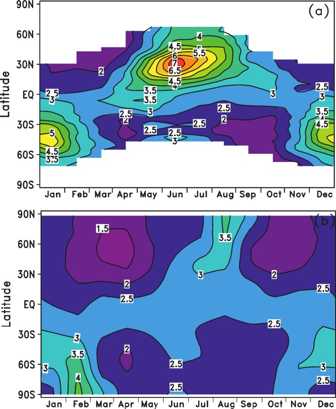
Mg⁺ column abundance (10⁹ atoms cm^–2) as a function of latitude and month: (a) observations using the Mg⁺ line at 279 nm in the dayglow; (b) WACCM-Mg model results, averaged from 2004 to 2011.¹⁷⁹

3.2.3. Nightglow Observations

There have been three novel developments during the past decade relating to the terrestrial nightglow.

First, nightglow spectra measured by both OSIRIS¹⁹⁰ and the ESI spectrometer on the Keck II telescope in Mauna Kea, HI,¹⁹¹ show that underlying the strong nightglow features between 540 and 680 nm from O, OH, and Na there is a quasi-continuum with maximum intensity at 595 nm (Figure 21). The same feature was observed in the spectrum of a persistent Leonid meteor train.¹⁹² Comparison with laboratory spectra shows that this emission arises from the “orange arc” bands of FeO:¹⁹³

R37

Reaction R37 is exothermic by about 300 kJ mol^–1, enough to generate FeO in several excited states (designated as FeO*). Figure 21 also shows a laboratory spectrum of the FeO arc bands, which was obtained at a total pressure of 1 mbar.¹⁹² The laboratory spectrum has been red-shifted by 5 nm to optimize the fit to the nightglow spectrum, which may indicate that at the lower pressure of the emission region around 87 km the population of emitting vibrational levels (and even electronic states) of FeO is somewhat different from that in the laboratory. The radiative lifetime of FeO* is 400 ns, which is about 4 times longer than the collisional lifetime in the laboratory experiment, but much shorter than the ∼200 μs collisional lifetime in the upper mesosphere; hence, significant collisionally induced vibrational development can occur in the laboratory.¹⁹⁴ The temporal behavior of the FeO emission is normally closely correlated with the 589 nm Na emission and the underlying OH(8–2) Meinel band (these are the much stronger features in Figure 21). The integrated intensities of the FeO, Na d, and OH(8–2) bands are ∼80, 21, and 260 R (where 1 R (Rayleigh) = 10⁶ photons cm^–2 s^–1). Although a 1-D model of Fe in the MLT satisfactorily reproduced the height and width of the FeO airglow layer,¹⁹¹ the intensity of 80 R could only be matched by assuming a 100% photon yield from reaction R37, whereas West and Broida¹⁹³ reported a yield of only around 2%. This is a substantial discrepancy which remains to be resolved.

Figure 21.

Nightglow spectrum (light gray line) between 500 and 700 nm recorded on the ESI spectrometer on the Keck II telescope in Mauna Kea, HI.¹⁹¹ The spectrometer has a resolution (λ/Δ) of 7000 and a wavelength accuracy of 0.005 Å. The red line is a laboratory spectrum of the FeO “orange arc” emission bands,¹⁹² red-shifted by 5 nm, which may indicate different vibrational development of the excited state(s) of FeO involved in the emission.

The second development in nightglow spectroscopy is emission from electronically excited NiO, detected at wavelengths longer than 440 nm in spectra from both OSIRIS and the GLO1 instrument flown on the Space Shuttle.¹⁹⁵ Although the emission is a very faint continuum compared with the FeO emission (which is to be expected since the Ni/Fe ratio in meteorites is around 6%), it is reasonably well-matched by laboratory spectra generated by the reaction of Ni atoms with O₃. The emission also peaks around 87 km. Surprisingly, the NiO*/FeO* emission ratio varies from 0.05 to 0.3.¹⁹⁵

The third development was the surprising observation that the ratio of the Na d lines at 589.0 and 589.6 nm in the terrestrial nightglow, R_D, is quite variable.^196−199 High-resolution airglow spectra taken with the Keck telescope in Hawaii reported that R_D varied between ∼1.3 and 1.9.¹⁹⁶ Measurements with an airborne spectrometer flying between 40° and 50° N during November 2002 found that R_D varied between ∼1.4 and 2.0 (average 1.8), changing over horizontal distances of 50–100 km.¹⁹⁷ Most recently, a large database of measurements of R_D was gathered at three locations: Andenes (Norway, 69° N), Kuujjuarapik (Canada, 55° N), and the Danum Valley (Borneo, 8° N). As shown in Figure 22a, R_D varied between 1.5 and 2.0, with an average value of 1.67. This variability is not explicable with the original Chapman mechanism for the Na d emission.²

Figure 22.

(a) Histogram of the occurrence frequency of Na d line ratio measurements. A total of 706 measurements were made between Oct 7 and Nov 19, 2007. The solid line is a fitted three-parameter Gaussian. (b) Correlation diagram for the electronic potential energy surfaces connecting the reactants NaO(A) + O and NaO(X) + O with the products Na + O₂, through the NaO₂ intermediate. Quartet surfaces have been omitted for clarity; these are highly repulsive states which do not influence the electronic nature of the products. (c) Laboratory study of the dependence of R_D on the ratio [O]/[O₂]. The experimental data (solid points) are from Slanger et al.¹⁹⁶ The solid line is a fit using the reaction scheme R38–R41. Adapted with permission from ref (198). Copyright 2012 Elsevier.

A laboratory simulation of the nightglow chemistry showed that R_D varies with the ratio of [O] to [O₂] over a range typical of the mesosphere. This led to the following modified Chapman mechanism being proposed:¹⁹⁶

R38

R39a

R39b

R40

R41a

R41b

In this scheme, reaction R38 makes excited NaO(A²Σ) exclusively, as shown in the laboratory.² Reaction R39 then produces Na(²P_J) with a branching ratio f_A and the two spin–orbit states in the ratio R_A (=[Na(²P_3/2)]/[Na(²P_1/2)]. Since the fluorescence lifetime of Na(²P_J) is very short (16 ns), there is no collisional mixing of the nascent state distribution at the very low pressures (<10^–5 bar) of the upper mesosphere. Hence, if only reactions R38 and R39 were involved, R_D would equal R_A. However, NaO(A) appears to be quenched efficiently to NaO(X) by collision with O₂, since there is near-resonant electronic-vibrational energy exchange.¹⁹⁶ NaO(X) then reacts with O, producing Na(²P_J) with a branching ratio f_X and with a ratio R_X between the spin–orbit states. The observed d line ratio R_D is then governed by competition between reactions R39 and R40 and should vary between R_A and R_X. A laboratory study (section 4.1) showed that R_D increases with [O]/[O₂], which implies that R_A > R_X.

This mechanism is further supported by a recent study which used a very high resolution Faraday filter spectrometer to determine the Doppler width of the d lines, as well as R_D, in the nightglow.¹⁹⁹ Since excited NaO(A) is 1919 cm^–1 above the ground state, Na(²P_J) atoms produced by reaction R39a are likely to have more kinetic energy than those produced by reaction R41a and hence larger Doppler widths. Harrell et al.¹⁹⁹ showed that the Doppler widths were indeed larger when R_D was higher.

These results were then interpreted using a theoretical model¹⁹⁸ of the Na nightglow which considered the statistical correlation of the electronic potential energy surfaces connecting the reactants NaO(A) + O and NaO(X) + O with the products Na + O₂, through the Na⁺O₂^– ion pair intermediate. The correlation diagram is illustrated in Figure 22b. Electronically excited NaO(A²Σ) is produced from the reaction between Na and O₃, followed either by reaction with O to generate Na(²P_J) with a branching ratio of 1/6 and a J = 3/2 to 1/2 propensity of 2.0 or quenching of NaO(A) to NaO(X²Π) by O₂. The resulting NaO(X) then reacts with O to generate Na(²P_J) with a branching ratio of 1/6 and a J = 3/2 to 1/2 propensity of 1.5. R_D should therefore vary between 1.5 and 2.0, as observed (Figure 22a).

In the context of the Na nightglow, it should be noted that a new retrieval method for satellite remote sensing of the global Na layer during nighttime has been proposed.²⁰⁰ The method would use satellite limb-scanning observations of O₃ density, temperature, and the Na d volume emission rate to retrieve the Na density. In their study, Xu et al.²⁰⁰ showed that the systematic retrieval error at the peak of the Na layer would be very small (less than 1%) and that most of the retrieval error would arise from uncertainties in the measurements of O₃, temperature, and the Na d volume emission rate. However, now that the mechanism for d line emission (reactions R38–R41) has been shown to be more complicated than the original Chapman mechanism assumed by Xu et al., the inherent uncertainty in this method probably needs to be re-examined.

3.3. Observations of MSPs in the Atmosphere and at the Surface

MSPs form via the polymerization of molecules such as FeOH, Mg(OH)₂, NaHCO₃, and SiO₂, which are the relatively long-lived reservoir metallic species on the underside of the metallic layers. Laboratory studies (described in section 4.3) have shown that these molecules polymerize rapidly, particularly if they contain Fe so that their collisions are governed by long-range magnetic dipole forces.^201−203 Nevertheless, because of their relatively low concentrations, polymerization occurs over several days and most of the particles around 80 km are just large molecular clusters, around 1 nm in effective radius. It has therefore proved challenging to detect them directly in the middle atmosphere and even harder to determine their composition. This has been frustrating given the potentially important roles that MSPs may play in the middle atmosphere: acting as ice nuclei for PMCs, affecting the balance of odd oxygen (O and O₃) and hydrogen (OH, HO₂) species through heterogeneous chemistry, playing an important role in the mesospheric charge balance, and as a significant component of stratospheric sulfate aerosol and polar stratospheric clouds, with possible impacts on the stratospheric O₃ layer.²

The aim of the MAGIC (Mesospheric Aerosol—Genesis, Interaction and Composition) project was to develop a rocket-borne instrument to sample MSPs in the mesosphere and return them to the ground for detailed analysis in the laboratory.²⁰⁴ MAGIC samplers, which exposed transmission electron microscopy grids in succession as the payload traversed the upper mesosphere, were flown on several sounding rocket payloads between 2005 and 2011. Hedin et al.²⁰⁴ have recently described the inherent challenges, both in sampling nanometer-sized particles and in their subsequent analysis. Although particles with compositions close to that expected for MSPs were found, problems with different types of contamination and uncertainties in the sticking efficiency of the particles on the sampling surfaces rendered the results inconclusive.

More successful has been the detection of charged MSPs using Faraday cup detectors on sounding rocket payloads.^{125,205−217} Faraday cup detectors are designed to collect charged particles, making use of the rocket payload’s ram velocity to drive the particles through a series of ground, bias, and rejection screens at the front of the detector. The rejection screen is used to prevent the collection of thermal electrons with energies below ∼1 eV, and the collecting anode is biased to a few volts positive in order to reject positive ions. Several assumptions are necessary to derive the charged dust particle density from the measured current. These include the following: all the thermal electrons are rejected, negative ion species are of low enough concentration to be an insignificant contribution to the measured current, and the MSPs are charged negative through the attachment of only one electron.²¹⁸ The function of rocket-based Faraday cup detectors can be severely hampered by aerodynamic flows, pressure buildup, and particle entrainment in and around the device.²¹⁹ A Monte Carlo collision model is typically used to determine the instrumental collection efficiency for the specific payload trajectory. The model requires an assumption about the particle density in order to determine the size range—typically between 0.5 and 2 nm radius depending on the payload velocity—that will be collected efficiently.^125,208,219

Figure 23 shows results from a recent study at Andøya, Norway (69° N), which employed a rocket-borne payload to measure charged MSPs, positive ions, electrons, and atomic O, together with ground-based lidar measurements of the Na density and temperature.¹²⁵ The payload passed within 2.6 km of the lidar beam at a height of 90 km, so that these are the first essentially collocated measurements of Na and O atoms in the MLT. As shown in Figure 23a, there is a close correspondence between the atomic O shelf below 90 km and the underside of the Na layer, as expected from the knowledge of Na chemistry (see section 3.1).

Figure 23.

Rocket-borne study of the Na layer and charged MSPs. (a) Comparison of the atomic O profile measured by the NEMI instrument on the HotPay 2 rocket payload, with the Na density measured by the ground-based ALOMAR Na lidar 5 min before the rocket launch. The payload passed within 2.58 km of the lidar at an altitude of 90 km. (b) Comparison of the profiles of positive ions and electrons measured by an ion probe and Faraday rotation technique on HotPay 2, compared with the predictions of the plasma model (including a profile of negative ions). The removal of electrons between 80 and 90 km is due to the charging of MSPs. (c) Vertical profile of negatively charged aerosols measured by a dust detector on HotPay 2, compared with the prediction from the dusty plasma model. The difference between the measured positive ions and electrons in (b) is also shown. Adapted with permission from ref (125). Copyright 2014 Elsevier.

Figure 23b illustrates a phenomenon in the plasma of the upper D region that has been known for many years: below about 90 km electrons become very depleted relative to positive ions, whereas they are in charge balance above this altitude.²¹³ Originally this depletion was explained by the formation of negative ions, which occurs via electron attachment to O₂⁷

R42

or dissociative electron attachment to O₃

R43

However, atomic O destroys the resulting negative ions before they can react further to form more stable anions such as NO₃^– and HCO₃^–:

R44

R45

A simple steady-state calculation shows that negative ion formation is shut down in the MLT when [O] > ∼1 × 10¹⁰ cm^–3, i.e., above 80 km (Figures 4a and 23a). In contrast, electronic structure calculations¹²⁵ show that electrons attach strongly to embryonic MSPs around 0.5 nm in radius containing Si (i.e., olivines and pyroxenes; see Figure 24b for examples), with binding energies of 2–3 eV, which reflects the stability of the SiO₃^– core ion.²²⁰ These energies are significantly larger than the electron affinity of O (1.46 eV), so that O atoms will not charge exchange with negatively charged MSPs. Furthermore, the rate coefficient for electron attachment to these small MSPs was calculated using Rice–Ramsperger–Kassel–Markus (RRKM) theory to be ∼4 × 10^–7 cm³ s^–1, which is roughly 10 orders of magnitude faster than electron attachment to O₂ (reaction R42) at the pressures of the upper mesosphere. Although the use of RRKM theory to predict the rate of an electron attachment reaction should be treated with caution in the absence of experimental data,^221,222 the estimated rate coefficient (which is similar to that for electron attachment to SF₆^221,222) appears to validate earlier proposals that the presence of heavy negative ions²²³ and electron depletion²⁰⁹ between 80 and 90 km is due to electron attachment to MSPs. This topic is also discussed in an accompanying review.²²⁴

Figure 24.

MSP work function. (a) Photoelectron currents measured during the flight of rocket payload ECOMA08. Black, green, and red symbols indicate the currents produced by the three different flashlamps (see the legend), where FX1162, FX1161, and FX1160 have cutoff wavelengths at 110, 190, and 225 nm, respectively. The dotted horizontal line marks the 2σ noise level of the unsmoothed measurements. (b) Optimized geometries of possible embryonic meteoric smoke particles: (FeOH)₄, (MgOH)₄, (FeSiO₃)₃, and (Mg₂SiO₄)₄. The vertical ionization potentials are shown alongside each cluster. Note that these are 2 eV larger when the cluster contains a silicon atom. Adapted with permission from ref (215). Copyright 2012 Copernicus Publications on behalf of the European Geosciences Union.

A model of Na chemistry (Table 1), MSP formation, and charging was used to show that the atomic Na layer and the vertical profiles of negatively charged MSPs, electrons, and positive ions can be modeled self-consistently using the same meteoric ablation flux.¹²⁵ Figure 23b shows the modeled and measured ion and electron profiles, and Figure 23c compares the measured profile of negatively charged MSPs with the model prediction for the relevant MSP size range. Note that the model predicts that around 6% of these small MSPs are charged between 80 and 90 km. Thus, the total MSP density is estimated to be about 16 times larger: that is, while Faraday cup measurements confirm the presence of MSPs, quantifying their total number density and size distribution is dependent on models which contain a significant number of poorly known parameters—polymerization and coagulation rates, charging properties, etc. This is a challenging problem because the plasma density in the D region is similar to the number density of MSPs (100–5000 cm^–3), rather than one or the other being in a significant excess.

An interesting development in the past 10 years has been the ECOMA (existence and charge state of meteoric smoke particles in the middle atmosphere) particle detector.²¹⁶ This is a Faraday cup instrument which contains up to three pulsed VUV lamps to photodetach electrons from negatively charged particles or photoionize neutral particles. One significant result has been to show that the resulting photoelectron current is proportional to the MSP volume density, and this property has been used to support global modeling predictions (see section 5.3) regarding the seasonal variability of MSPs.²¹¹

When the ECOMA detector employs three flashlamps, each lamp has a different window material with a different cutoff wavelength. Figure 24a shows the measured photoelectron currents from the three lamps as an ECOMA payload ascended from 70 to 95 km. Flashlamp FX1162, with a cutoff at 110 nm, produces a much larger photoelectron current compared with the other lamps with cutoffs at 190 and 225 nm, particularly above 88 km. These data enable constraints to be placed on the MSP size, work function, and composition. For instance, the particles observed in Figure 23a were concluded to be in the 0.5–3 nm size range, increasing in size toward lower altitudes (as expected due to coagulation). The MSP work function was estimated to be in the range from 4 to 4.6 eV. Electronic structure calculations (Figure 23b) were used to show that this low work function indicates that iron and magnesium oxy/hydroxide clusters, rather than metal silicates, were the major constituents of the MSPs producing the photoelectron currents measured on this flight.²¹⁵

Another significant conclusion from a series of ECOMA flights conducted around the Geminids meteor shower is that the column density of negatively charged MSPs correlated well with the sporadic meteor flux measured by radar during the same period, rather than the shower meteors. This implies that the sporadic meteors are the major source of MSPs, while the additional influx from a strong meteor shower did not make a significant contribution.²¹⁵

MSPs have also been detected from the distinctive line shapes of incoherent scatter radar spectra which result from the different diffusion modes in the D region plasma caused by the presence of positive ions and relatively heavy negatively charged MSPs.²²⁵ The technique allows MSP number densities and size to be retrieved, although the approximation of a monodisperse MSP population has to be assumed. Most of the work has been performed with the 430 MHz dual-beam Arecibo incoherent scatter radar in Puerto Rico (18° N).²²⁶ MSP radii between 0.6 and 1.5 nm and number densities of 10²–10⁴ cm^–3 were determined in the 80–95 km height range, depending on the altitude and season. More recently, this approach has been used with the Poker Flat, AK, coherent radar at 65° N.²²⁷

Within the past 5 years, MSPs have also been detected by optical extinction from the limb-scanning Solar Occultation for Ice Experiment (SOFIE) spectrometer on the Aeronomy of Ice in the Mesosphere (AIM) satellite.²²⁸ Figure 25 shows the MSP extinction at 1.037 μm measured from ∼40 to 75 km altitude. The key to this measurement is the extremely small extinctions of <1 × 10^–8 km^–1 that can be measured by SOFIE because of the bright solar light source and a path length of ∼300 km through the atmosphere. The extinction measurements have a vertical resolution of ∼2 km. As expected because of the meridional circulation in the mesosphere, a seasonal cycle was observed with a reduced MSP abundance during polar summer (see section 5.3).

Figure 25.

Comparison of measured MSP extinction (labeled SOFIE/AIM) with values calculated using MSP number concentrations from the UMSLIMCAT model and Rayleigh theory for an assumed olivine (MgFeSiO₄) composition and for the same pyroxene (Mg_0.4Fe_0.6SiO₄) species used to fit the SOFIE data by Hervig et al.²²⁸ Also shown are the predicted MSP extinction profiles from the WACCM²⁷⁸ and CHEM2D²⁷⁷ models. Reprinted with permission from ref (279). Copyright 2012 Copernicus Publications on behalf of the European Geosciences Union.

Hervig et al.²²⁸ used the predicted MSP distributions in the stratosphere and mesosphere from 2-D and 3-D models to compute the extinction profiles for a variety of different particle compositions, using published mineral refractive indices. The best fit to the SOFIE observations was obtained with a mixed pyroxene composition, Mg_0.4Fe_0.6SiO₄ (Figure 25). In a subsequent study, Hervig et al.²²⁹ studied the extinction due to PMCs at four wavelengths from the UV to the mid-IR (0.330, 0.867, 1.037, and 3.064 μm) and showed that the extinction was inconsistent with pure H₂O ice particles. Instead, they proposed that the PMC particles contain significant amounts of meteoric smoke (0.01–3% by volume). The smoke extinction at the four wavelengths was also shown to be consistent with metal oxides such as FeO and Mg_xFe_1–xO (x = 0.1–0.6), rather than pyroxene. Interestingly, the absence of silicon is consistent with the smoke composition deduced from the low work functions of MSPs measured by the ECOMA instrument (see above).²¹⁵

Recently, the accumulation of meteoric material in the lower stratosphere during the Arctic winter has been measured with a four-channel condensation particle counter on an aircraft flying up to 20 km.^230,231 Inside the polar vortex up to 75% of aerosol particles can contain refractory material, i.e., thermally stable residuals with diameters from 10 nm to a few micrometers which endure heat exposure at 250 °C. The fraction of nonvolatile particles correlates inversely with the atmospheric N₂O concentration, which indicates that the refractory aerosol originates from the upper stratosphere/mesosphere. These refractory cores are almost certainly MSPs which are transported downward by the prevailing meridional circulation (Figure 1 and section 5.3). By comparing campaigns over a number of years with different vortex strengths, it is clear that these large concentrations of refractory aerosol are a regular feature at the base of the polar vortex, with the accumulation starting during December and reaching its highest level during March in the Arctic.

MSPs are deposited at the Earth’s surface 4–5 years after formation in the MLT.²³² Several studies in the past decade have reported measurements of the MSP deposition flux in polar ice cores. In the first of these, Gabrielli et al.²³³ measured the concentration of Ir and Pt in the Greenland Ice Core Project (GRIP) ice core from Summit, central Greenland (72° N), using inductively coupled plasma sector field mass spectrometry (ICP-MS). Low and remarkably constant concentrations were recorded in the Holocene (the current geological period) for both Ir and Pt (averages of 0.3 and 0.6 fg g^–1 of ice, respectively), compared with higher and more variable values (averages of 2 and 3 fg g^–1) during the last glacial age (LGA), approximately 110,000−12,000 years ago. By combining these measured concentrations with the snow accumulation rate, the average deposition fluxes of Ir and Pt during the Holocene were 8 and 15 fg cm^–2 year^–1, respectively, a factor of 2–3 lower than those during the LGA (24 and 32 fg cm^–2 year^–1). The higher flux during the LGA was because of an increased deposition of crustal dust (lower sea levels caused exposure of coastal seabed sediments, resulting in a dustier atmosphere). To correct for the crustal contribution, the Ir and Pt signals were normalized to Al measured in the ice, which is an element that is a good indicator of crustal dust. This showed that the contribution from crustal dust to the fluxes of Ir and Pt during the Holocene was negligible and that the ratio of these elements was in the expected cosmic abundance (Ir/Pt = 0.49), confirming that they were of extraterrestrial origin.

In a follow-up study, Ir and Pt were measured in deep Antarctic ice from EPICA/Dome C (75° S) and Vostok (78° S).²³⁴ A low meteoric accretion rate during glacial periods was observed, being about 4 times lower than in central Greenland. However, in interglacial (warm) periods the ratios of these elements was superchondritic (Ir/Pt ≈ 1), possibly because of volcanic fallout of Ir-rich dust transported by the prevailing interglacial circulation to the eastern highlands.²³⁴

Another method for detecting MSPs in polar ice cores is laboratory-induced remanent magnetization, which measures the magnetization carried by ferromagnetic dust particles in the ice.^235−237 This nondestructive technique provides a way of separating MSPs from larger crustal dust particles. The ice sample is exposed to a strong magnetic field, which induces a remanent magnetic field present in the sample after it is removed from the field. The remanent field will decay if there is thermal relaxation of the aligned magnetic particles to an equilibrium state. The particles that become unstable with increasing temperature are termed superparamagnetic. Lanci and co-workers^235−237 applied this technique to the same ice cores as used for the previous studies on Ir and Pt.^233,234 The decay of the remanent field was measured by warming each ice sample from 77 to 255 K. Over this temperature range, particles with radii between 3.5 and 10 nm become superparamagnetic and account for the measured fractional loss of magnetization. In the case of central Greenland during the Holocene, the concentration of superparamagnetic Fe was almost identical to that calculated from the Ir and Pt measurements using the relative Fe/Ir and Fe/Pt cosmic abundances. In the case of EPICA/Dome C and Vostok, the superparamagnetic Fe concentration was within the uncertainty of the Fe concentration estimated from the Ir and Pt measurements, though only during glacial times (supporting the hypothesis of Gabrielli et al.²³⁴ that volcanic fallout contaminates the MSP Ir/Pt signal during warm periods). Lanci et al.²³⁵ have provided convincing evidence that wet deposition of the ultrafine MSPs is much more important than dry deposition and showed that the deposition flux is about an order of magnitude higher in central Greenland than the eastern highlands of Antarctica, consistent with the relative snowfall at the two locations.

4. Laboratory and Theoretical Studies

As discussed in the previous section, the metallic species that are directly measured in the MLT are the neutral atoms and atomic ions, and some information is starting to be acquired about the composition of MSPs. This means that knowledge of the atmospheric chemistry that gives rise to the metal layers, and the nature of the metal-containing reservoir species that polymerize into MSPs, has to be derived from a combination of experimental laboratory studies, theory, and modeling.

4.1. Gas-Phase Chemistry of Metallic Species

The two classical techniques of flash photolysis and the fast flow tube have been applied with great success to the challenging task of studying reactions of neutral and ionic metallic species in the gas phase at the low temperatures characteristic of the upper atmosphere. Previous reviews¹⁻⁴ have described the application of these techniques in some detail, so here there will be a brief description of the experimental methodology followed by a focus on studies during the past decade.

Figure 26a is a schematic diagram of a pulsed laser photolysis/laser-induced fluorescence (PLP/LIF) system, in this case for studying the reaction of Mg⁺ ions with O₃.¹⁰⁵ Mg⁺ was produced by the multiphoton photolysis of a gas-phase precursor molecule, MgAcAc (formula Mg(C₅H₇O₂)₂), using a focused excimer laser at 193 nm. The MgAcAc vapor was produced by heating a solid sample of MgAcAc to around 450 K in a tantalum boat located in a heat pipe connected to the central reaction chamber (Figure 26a). The resulting Mg⁺ ions were then followed by time-resolved LIF of Mg⁺ at 279.6 nm (Mg⁺(3²P_3/2–3²S_1/2)), in the presence of a known concentration of O₃ which was measured by absorption at 254 nm at the exit of the reaction chamber. The decay of Mg⁺ ions is very well fitted by a single exponential (Figure 26b), which gives the first-order loss rate. By varying the reagent concentration (O₃ in this case), the rate coefficient was determined.¹⁰⁵

Figure 26.

(a) Schematic diagram of the pulsed laser photolysis/laser-induced fluorescence detection apparatus used to study the reactions of Mg⁺ ions. The metal precursor (magnesium acetyl acetonate) is placed in a tantalum boat in the side arm of the reactor. PMT = photomultiplier tube, MC = monochromator, PD = photodiode, and BE = beam expander. (b) Time-resolved profile of the LIF signal obtained by pumping the Mg⁺(3²P₁)–Mg⁺(3¹S₀) transition at 279.6 nm and monitoring emission at the same wavelength, following the pulsed photolysis at 193.3 nm of magnesium acetyl acetonate. The solid line is a fit to the form A exp(−k′t).

The PLP/LIF technique has been applied in our laboratory since 2004 to study the reactions of Ca⁺ ions¹⁰⁶ and Mg⁺ ions^105,108,238 with O₃, O₂, N₂, CO₂, N₂O, and H₂O at temperatures down to 195 K. This technique has also been used to study the reactions of Si atoms with O₂, O₃, CO₂, and H₂O⁹⁷ and SiO reactions with O₃ and OH.⁹⁸ Most recently, this system has been used to study the reactions of Na, K, Mg, and Fe with NF₃, an industrial gas with a very large global warming potential because of its atmospheric lifetime of ∼550 years, which enables it to reach the mesosphere.²³⁹

The fast flow tube technique is particularly useful for studying the reactions of metal-containing molecules, both neutral and ionic, with unstable reagent species. Figure 27 illustrates a fast flow tube apparatus used to study the reaction kinetics of the neutral species CaO, CaO₂, CaO₃, CaCO₃, and Ca(OH)₂ with O and H.¹⁰⁹ Ca atoms were produced thermally in the upstream section of the tube and then appropriate reagents (e.g., N₂O, O₂, CO₂, and H₂O) added downstream (through injection ports I2 and I3 in Figure 27). Further downstream, atomic O made by the microwave dissociation of N₂ followed by titration with NO, or H made by the microwave dissociation of H₂, was added in a known excess measured by chemiluminescence at the first photomultiplier port. Ca and CaO were monitored by LIF at 422.7 nm (Ca(4¹P–4¹S)) and 385.9 nm (CaO(B¹Π–X¹Σ)). Extracting rate coefficients from this complex reaction system requires a full kinetic model of the flow tube, including diffusional losses to the walls of all these reactive species (the diffusional loss rates need to be measured separately).¹⁰⁹ This flow tube apparatus has also been used to study the reactions of FeO, FeO₂, and FeO₃ with O, and FeOH with H, where Fe is produced by the pulsed ablation of an Fe target using a 532 nm Nd:YAG laser.¹¹⁷ More recently, the reactions of MgO, MgO₂, OMgO₂, and MgCO₃ with O have been studied, using thermal production of Mg vapor.¹¹⁶

Figure 27.

Schematic diagram of a fast flow tube apparatus used to study the reactions of neutral Ca (probed by LIF at 422.7 nm) and CaO (probed by LIF at 385.9 nm). P = photomultiplier tube. I1, I2, and I3 are reagent inlets.

The flow tube technique has also been used to investigate the reactions of ionic metal-containing species. These species were monitored at the downstream detection point by a quadrupole mass spectrometer (Figure 27). The reactions of Si⁺ and SiO⁺ with O₃ and O₂ were studied by using pulsed laser ablation of a crystalline Si rod to produce Si⁺ in the upstream section of the flow tube.⁹⁹ Ca⁺ ions were produced by ablation of a calcite (CaCO₃) target, and this source was used to study the reactions of CaO⁺ with O and CO and a variety of switching reactions between cluster ions with O₂, CO₂, and H₂O ligands.²⁴⁰ Mg⁺ ions were produced by ablation of a magnesite (MgCO₃) or MgO target and used to study the reactions of MgO⁺ and MgO₂⁺ with O, as well as ligand-switching reactions with CO₂ and O₂ (also relevant to the Martian mesosphere).^105,108

Flow tubes have also been used to explore the reaction kinetics of O₂(a¹Δ_g) with Si⁺ ions¹²² and Mg, Fe, and Ca atoms.¹¹⁵ As discussed in section 3.1, this first excited state of O₂ is produced in the MLT by the photolysis of O₃ and during daytime has a concentration about 30 times higher than that of O₃. O₂(a) was prepared using a new technique where Cl₂ is bubbled through a chilled alkaline solution of H₂O₂, producing O₂(a) at up to 30% yield:

R46

The O₂(a) concentration was determined in these experiments by measuring the weak emission at 1270 nm from O₂(a–X) emission with an InGaAs photodiode detector; the absolute sensitivity of the light collection, transmission, and detection was determined using a radiometric calibration standard.^115,122

The variability of the Na d line ratio, R_D, was discussed earlier in section 3.2.3. To understand the atmospheric observations, a laboratory study¹⁹⁶ was carried out using a flow tube similar to that in Figure 27, but with a liquid N₂ cooling jacket to operate over the temperature range of 90–300 K. At the upstream end, gas-phase Na atoms were produced in an oven, entrained in a flow of N₂, and injected into the cooled section of the flow tube. Flows of O, O₃, and O₂ were then introduced to generate Na chemiluminescence via reactions R38–R41, and R_D was measured at the downstream end of the tube as a function of the ratio [O]/[O₂]. As shown in Figure 22c, R_D is equal to the measured atmospheric average value of 1.67 (Figure 22a) when [O]/[O₂] is ∼2 × 10^–3 and increases to 2.0 when [O]/[O₂] approaches 1 × 10^–2. These ratios correspond to atmospheric nighttime O concentrations at about 86 and 90 km, respectively, which encompass the Na d emission height range. The solid line in Figure 22c is a fit of the statistical correlation model (section 3.2.3) to the data which indicates that k₄₀, the rate coefficient for the quenching of NaO(A) by O₂, is ∼1 × 10^–11 cm³ molecule^–1 s^–1.¹⁹⁸

Finally, an important gap in the current knowledge of metal ion–molecule chemistry is kinetic studies of DR reactions of metal-containing molecular ions. In fact, the only relevant reaction that appears to have been studied is the DR of Na⁺·D₂O cluster ions. The energy dependence of the reaction cross-section was measured in the former CRYRING facility in Stockholm (Sweden), from which the temperature-dependent rate coefficient was computed.²⁴¹

4.2. Ice Chemistry of Metallic Species

The observed removal of Fe, Na, and K metal atoms in the vicinity of PMCs has been discussed in section 3.2.1. To model this phenomenon, uptake coefficients (γ) of these atoms on ice were measured in the laboratory using a low-temperature flow tube.¹³⁵ The flow tube had an outer jacket to allow the pulsed circulation of liquid N₂ with a feedback loop so that the temperature of the tube could be controlled between 80 and 150 K. Measurements of the uptake of the metals were made on ice films of both amorphous and cubic crystalline phases, which are the two metastable phases of ice that should exist at mesospheric temperatures and pressures. A film of amorphous ice (thickness ∼20 μm) was produced by deposition of H₂O from a sliding injector onto the tube walls at about 90 K and then annealed at higher temperature to control the phase and morphology. The ice films were extensively characterized using the BET isotherm technique.²⁴² These measurements showed that the surface area of freshly deposited ice at 90 K was around 2500 times larger than the geometric surface area and that this surface area enhancement decreased to just 90-fold if the ice film was annealed at 160 K.

Metal atoms were produced in the upstream part of the tube, either thermally (Na and K) or by pulsed laser ablation of an Fe rod. The uptake of all three metals was found to be highly efficient and mostly in the diffusion-limited regime, which then required accurate measurements of the diffusion coefficients of the metal atoms in He (this carrier gas is used because diffusion to the walls is about 3 times faster than in N₂). The uptake of Fe on cubic ice is close to unity efficiency above 135 K, but γ(Fe) decreases to only 3 × 10^–3 on cubic ice at 80 K. In contrast, uptake of Fe on amorphous ice films is much more efficient (γ(Fe) > 0.1). Quantum calculations of the Fe atom adsorbed onto a 12 H₂O molecule model ice surface show that the Fe bonds strongly to lone pairs on the oxygen atoms in the H₂O molecules exposed at the surface.¹³⁵ Above about 130 K the surface molecules of ice are sufficiently mobile to rotate and accommodate the Fe–O bond, leading to very efficient uptake. However, at lower temperatures the rigidity of the ice surface increasingly prevents this. In contrast, uptake on amorphous ice is large even at very low temperatures because the disordered ice surface will have exposed and therefore accessible O atoms. γ(Na) and γ(K) were larger than 0.1 on both types of ice between 80 and 150 K.

Although rocket-borne measurements have confirmed that there is usually a “bite-out” in the electron density profile in the vicinity of a PMC (which gives rise to PMSEs, section 2.3), charged particle collectors on rockets have also shown that on rare occasions PMC particles can be positively charged, with an enhanced cloud of electrons around them.^243,244 Photoionization of ice particles is one potential mechanism for the generation of these positively charged particles. However, at heights below 100 km in the atmosphere there is insufficient intensity in the solar spectrum of photons with energies greater than the work function of ice (8.7 eV). Indeed, attempts to simulate the experimental observations required the particles to have a work function on the order of 2.5 eV.²⁴⁵

Since PMCs occur between 83 and 95 km on the underside of the metal layers, and both lidar observations (section 3.2.1) and laboratory experiments (see above) show that metal atoms are readily taken up on low-temperature ice, the photoelectric emission from alkali-metal atoms deposited on ice has been measured.^246−248 The experiments were carried out in an ultra-high-vacuum chamber where photoelectron energies were determined with an electron time-of-flight spectrometer. A thick film of H₂O (∼3000 langmuirs) was dosed onto a Cu(111) substrate at 90 K, followed by Na, K, or Li so that no more than 2% of a monolayer of metal was deposited on the ice. The ice film was then irradiated with a pulsed low-energy visible laser. Figure 28 shows that the effect of Na deposition is to reduce dramatically the work function of ice to just 2.3 ± 0.2 eV, compared with 5.2 eV for a Na atom in the gas phase. Furthermore, the photoionization cross-section is enhanced by a factor of 30.

Figure 28.

Photoionization cross-section of Na atoms adsorbed on ice (black points and line),²⁴⁷ compared with gas-phase Na atoms (red line).³²⁸ The blue line is the solar photon flux (right-hand ordinate).

When the photoionization cross-section is integrated over the solar irradiance spectrum (also shown in Figure 28), the photoionization lifetime of a Na atom adsorbed on an ice particle in the mesosphere is about 10 s, compared with 5 × 10⁴ s for a Na atom in the gas phase. Similar substantial changes were observed for K and Li.²⁴⁶ The small work function and large photoionization cross-section of Na/ice therefore appear to be what is required to explain the occurrence of positively charged PMC particles.²⁴⁵ However, the laboratory study also showed that the initial state formed by freshly deposited metal atoms is metastable. In the case of Na/ice, the photoemission yield decreases at a rate of (4 ± 0.4) × 10^–4 s^–1 at 93 K, presumably as NaOH and H₂ form. Furthermore, this rate increases at higher temperatures with an activation energy of 10 ± 2 kJ mol^–1, so that at a typical PMC temperature of 135 K the metastable state with high photoelectric yield lasts for only ∼20 s (and even less time for K and Li). This means that a rapid uptake of fresh Na atoms would be required to sustain positively charged ice particles, which would only likely occur shortly after the ablation of a sizable meteoroid.

Bellan²⁴⁹ has proposed that the high radar reflectivity of PMSEs (section 3.3) can be explained by the ice grains being coated by a thin metal film produced by deposition of Fe and Na. Reflectivity would be generated by the large number of delocalized conduction electrons in the metal film, and it was argued that this would make a much larger contribution than the “classical” picture of plasma inhomogeneities around the ice cloud layer. This proposal has already generated a lively correspondence.^250−252 One further problem with it is that, as discussed above, the delocalized electrons generated by freshly adsorbed metal atoms will quickly disappear at PMSE-relevant temperatures as the metals react with the substrate to form metal hydroxides.

A very recent study²⁵³ using the UHV apparatus described earlier²⁴⁸ has explored two questions related to Fe uptake on PMC ice particles. First, temperature-programmed desorption measurements of an ice film coated with a submonolayer of Fe showed that no Fe atoms or Fe-containing species codesorbed along with the H₂O molecules. This implies that when PMC ice cloud particles sublimate, the metallic species embedded in them will coalesce to form residual (potentially large) smoke particles. Second, measurements of the ion-sputtering efficiency of Fe from the ice film were extrapolated to the conditions of an intense proton aurora, which indicated that the sputtering of Fe species from PMC ice particles into the gas phase will not compete with fresh injection from meteoric ablation.

4.3. MSP Formation and Atmospheric Impacts

The major elements injected into the MLT from meteoric ablation should be Fe, Mg, and Si in roughly similar quantities.⁹⁶ Laboratory kinetic studies have shown that these elements are oxidized in the presence of O₃, O₂, and H₂O to form reservoir species such as FeOH, Mg(OH)₂, and SiO₂ (sections 3.1 and 4.1). The next step in the passage of these meteoric vapors through the atmosphere is the formation of MSPs. A number of laboratory and theoretical studies^{201−203,254} have been performed in the past few years to elucidate the polymerization pathways for forming embryonic MSPs, measure polymerization rates, explore the composition and morphology of the particles, and measure their optical extinction for comparison with SOFIE observations (section 3.3). Figure 29 is a schematic diagram of an apparatus for the generation of MSP analogue particles, which were synthesized by the photo-oxidation of mixed vapors of the precursors iron pentacarbonyl (Fe(CO)₅), magnesium ethoxide (Mg(OC₂H₅)₂), and tetraethyl orthosilicate (Si(OC₂H₅)₄) with O₃ in N₂ bath gas at atmospheric pressure. A broad-band Xe arc lamp (λ > 300 nm) was used as the photolytic source. The generated particles were sampled downstream of the flow cell by inertial deposition onto holey carbon grids suspended in the gas flow, for subsequent analysis by transmission electron microscopy with energy-dispersive X-ray spectroscopy (TEM-EDX) and electron energy loss spectroscopy (EELS). The particle size distribution between 0.6 and 40.0 nm was measured with an electromobility spectrometer, comprising a differential mobility analyzer and a Faraday cup electrometer. Extinction measurements were performed using a White cell optical arrangement (total optical path length of ∼6 m).

Figure 29.

(a) Experimental system used for the photochemical generation, detection, capture and optical extinction measurements of MSP mimics. (b) Transmission electron microscopy images and an electron diffraction image taken from the indicated area within a smoke aggregate formed following the irradiation of a mixture of Fe(CO)₅, O₃/O₂, and tetraethyl orthosilicate. Adapted with permission from ref (201). Copyright 2006 Elsevier.

The EDX/EELS analysis shows that the particle composition resulting from the photo-oxidation of Fe, Mg, and Si precursor vapors was homogeneous in all cases, and the average particle compositions were consistent with olivine ([Mg_xFe_1–x]₂SiO₄, x = 0–1) and not pyroxene structures. Furthermore, the relative Fe/Mg composition in the particles can be controlled quantitatively from x = 0 (fayalite) to x = 1 (forsterite) by varying the relative flows of the organometallic precursors. Electronic structure calculations identified several highly exothermic pathways to form the basic metal silicate molecules in these particles and showed that these molecules would polymerize via even more exothermic reactions; hence, there should not be a free energy barrier associated with MSP formation.²⁰³

A modified flow reactor was used to study the fast kinetics of particle growth.²⁰¹ Coalescent growth leads to the formation of primary particles with a radius, r₀, around 6 nm.²⁰² Collisions between particles which are greater than or equal to r₀ in size then form fractal-like aggregates, as shown in Figure 29b. The growth of these aggregates when the primary particles contain Fe is much faster than can be modeled by conventional coagulation kernels assuming “hard-sphere” collisions. This is explained by the large capture frequency of two particles with randomly oriented magnetic dipoles.²⁰¹ Another point of interest is that when an excess of SiO₂ is present during the synthesis of olivine particles, separate amorphous silica particles form which grow only through coalescence (inset in Figure 29b). The measured optical extinction spectra of fractal-like particles with elemental compositions corresponding to fayalite (Fe₂SiO₄), goethite (FeOH), and hematite (Fe₂O₃) were satisfactorily modeled using Mie theory for a polydisperse distribution of spherical particles and the refractive index data for the bulk minerals (which is an important conclusion for interpreting satellite extinction spectra).²⁰¹

Amorphous Fe₂O₃ particles (modal diameter 30 nm) generated using the photochemical reactor were also investigated for their propensity to nucleate ice over the temperature range of 180–250 K, using the AIDA chamber in Karlsruhe, Germany.²⁵⁵ Ice formation via the deposition mode was initiated by ∼10% of these small particles at a threshold ice supersaturation of 140% and an initial chamber temperature of 182 K. Classical nucleation theory was used to determine a contact angle of θ = 10.5° with a slightly negative temperature dependence. Thus, although the Fe₂O₃ nanoparticles are relatively efficient ice nuclei for conditions which correspond to cirrus cloud formation in the upper troposphere, at the lower temperatures where PMCs form (<150 K) higher contact angles would be expected, which may reduce the effectiveness of these particles as ice nuclei in the MLT.²⁵⁵

However, as discussed in section 3.3, around 6% of MSPs should be negatively charged in the 80–85 km region, and the presence of even a single charge on a nanometer-sized particle can make it an effective PMC ice nucleus by reducing the classical free energy barrier associated with the Kelvin effect.²⁵⁶ In fact, particles larger than 1 nm may not be required as ice nuclei. Electronic structure theory calculations indicate that the neutral metal silicate molecules FeSiO₃ and MgSiO₃ should form readily in the upper atmosphere.²⁵⁴ These molecules, which may be regarded as the smallest smoke particles, have extremely large electric dipole moments of 9.5 and 12.2 D, respectively. H₂O molecules therefore bind very effectively to them, with Gibbs free energy changes in excess of −100 kJ mol^–1. Indeed, the addition of up to eight H₂O molecules occurs more favorably than the sublimation of H₂O to bulk ice. FeSiO₃ and MgSiO₃ should therefore nucleate ice particles under polar mesospheric conditions at temperatures around 140 K.²⁵⁴

5. Global Atmospheric Modeling of Meteoric Metals

This section describes the implementation of meteoric metal chemistry in a whole atmosphere chemistry climate model. To achieve this, three components are required. First is the meteoric input function (MIF), which specifies the injection rate of each element (Na, Fe, etc.) into the atmosphere as a function of time and latitude (section 5.1). Second, the modules of metal gas-phase chemistry (Tables 1–5) have to be added to the general atmospheric chemistry in the model. Third is the inclusion of a description of removal of the gas-phase species through the formation of MSPs. In section 5.2 the model results are compared with the observations already described in section 3.2. In sections 5.3 and 5.4, the impacts of MSPs in the stratosphere and at the Earth’s surface are discussed.

5.1. Chemical Model of Meteoric Ablation and the Meteoric Input Function

Because of their very high entry velocities, meteoroids undergo rapid frictional heating by collision with air molecules, and their constituent minerals subsequently vaporize. The physics of this process has been treated in detail by several investigators and is described in a previous review.² Frictional heating is balanced by radiative losses and by the absorption of heat energy through temperature increases, melting, phase transitions, and vaporization. To calculate these terms, parameters such as the meteoroid shape, density, and composition are needed (the current working assumption is that most of the extraterrestrial material has the composition of carbonaceous chondrites).

To understand ablation at the level of individual meteoric elements, a chemical ablation model (CABMOD) has been developed which includes the following processes: sputtering by inelastic collisions with air molecules before the meteoroid melts, evaporation of atoms and oxides from the molten particle, diffusion-controlled migration of the volatile constituents (Na and K) through the molten particle, and impact ionization of the ablated fragments by hyperthermal collisions with air molecules.⁹⁶

The mass loss rate is calculated using Langmuir evaporation, which assumes that the rate of evaporation into a vacuum is equal to the rate of evaporation needed to balance the rate of uptake of a species i in a closed system. The rate of mass release of species i with molecular weight μ_i, from a particle of area S, is then given by the Herz–Knudsen equation:

E2

where γ is the uptake coefficient, equal to the probability that the molecule is retained on the surface, or within the particle, after collision with the surface, and p_i is the thermodynamic equilibrium pressure of species i in the gas phase. The total mass loss rate due to ablation is then the sum over all gas-phase components i. High-velocity collisions with air molecules also cause the nonthermal sputtering of atoms from the surface of the meteoroid, which results in mass loss before the particle melts and thermal evaporation dominates. CABMOD includes a treatment of nonthermal interactions which uses a semiempirical model derived from experimental ion sputtering yields.²⁵⁷

The vapor pressures of the species evaporating from the meteoroid are calculated using the MAGMA chemical equilibrium code,²⁵⁸ which exhibits good agreement with experimental data for a wide range of temperatures and silicate melt compositions. MAGMA uses the ideal mixing of complex components and includes the equilibria of eight metal oxides: SiO₂, MgO, FeO, Al₂O₃, TiO₂, CaO, Na₂O, and K₂O. The chemical equilibria in the melt are modeled using thermodynamic activities, which are the product of the Raoultian activity coefficient of the oxide (relative to the pure liquid oxide) and the mole fraction of the oxide in the melt. The melt is treated as a nonideal solution in which the concentrations of the unbound metal oxides are reduced by the formation of complex oxides and pseudocomponents. The equilibria between components in the melt, and between the melt and vapor, are calculated simultaneously, and it is assumed that the oxides evaporate stoichiometrically. The vapor pressure of each gas-phase species is then used to determine the mass loss rate of that component from the melt by invoking Langmuir evaporation (eq E2). This approach is similar to the equilibrium reference model for evaporation into a vacuum from a silicate melt that was described by Alexander,²⁵⁹ which reproduced the measured elemental evaporation rates from chondritic-type melts over a temperature range of 1900–2300 K, for up to 95% mass loss.

Figure 30 shows the predicted ablation profiles of the major meteoric elements from a 5 μg meteoroid entering the atmosphere at 20 km s^–1. This clearly displays differential ablation, where the relatively volatile elements (Na and K) ablate about 10 km higher in the atmosphere than the main constituents (Fe, Mg, and Si), and the more refractory species (Ca, Al, and Ti; the latter two are not shown for clarity) ablate about 5 km lower. Note that the meteoroid melts when the temperature exceeds 1800 K at a height of 102 km. Above this height, metal atom injection is caused by sputtering, so the injection rates of all constituents decrease with the same (atmospheric) scale height.

Figure 30.

Ablation/sputtering profiles of individual elements from a 5 μg meteoroid entering the atmosphere at 20 km s^–1 and at 37° to the zenith. The particle temperature is shown with the solid black line, referenced to the top abscissa. Adapted with permission from ref (96). Copyright 2008 Copernicus Publications on behalf of the European Geosciences Union.

There are three ways that the prediction of differential ablation has been tested. First, differential ablation explains⁹⁶ the observation that when common-volume lidar measurements are made of two or three metals, meteor trails that pass through the common volume rarely contain more than a single metal: two metals are seen less than 1% of the time and three metals only once out of thousands of observed trails.²⁶⁰ The second piece of direct evidence comes from observations of meteor head echoes in high-performance large-aperture radars, such as the Arecibo 430 MHz instrument in Puerto Rico (18° N).²⁶¹ As an example, Figure 31a shows the range-time intensity of a meteor, with the measured velocity profile in panel b. The meteor head echo, plotted in panel c, shows a sudden burst of intensity around 106 km. CABMOD can be used to predict the injection profiles of the different elements, for a chosen meteoroid mass and entry angle (as in Figure 30). The model can also estimate the ionization efficiency of each type of metal atom colliding with air molecules at the hyperthermal velocity of the meteor.⁹⁶ The resulting total electron production rate along the meteor track can then be used to compute the head echo and the exercise iterated to get the best fit to the observations. Panel c shows that a very satisfactory fit can be achieved using the ablation profiles in panel e, for a meteoroid with a mass of 10 μg.²⁶¹ A third test for differential ablation is that CABMOD has been used to interpret quantitatively the measured depletion of elements in cosmic spherules recovered from sediments in the Indian Ocean.^262,263

Figure 31.

An observed meteor with the following best fit parameters: initial velocity 36 km s^–1; entry angle 1° (to zenith); mass 10^–8 kg; density 3500 kg m^–3. (a) Meteor range-time intensity, measured with the 430 MHz Arecibo radar. (b) Modeled (line) and observed (tilted squares) meteor altitude–velocity profile. (c) Modeled (black) and observed (red) meteor signal-to-noise ratio. (d) Modeled meteor radar cross-section. (e) Ablation profiles of the main elements (bottom axis) and total amount of electrons produced (upper axis), predicted by CABMOD.⁹⁶ The horizontal line across the plots shows that the observed enhancement in SNR is due to the rapid ablation of the alkali metals Na and K. Reprinted with permission from ref (261). Copyright 2009 John Wiley & Sons, Inc.

It should be noted that meteoroid entry into the atmosphere involves processes not currently included in CABMOD. In particular, fragmentation of meteoroids may be a relatively common event. For example, Malhotra and Mathews²⁶⁴ used the new Resolute Bay (Canada) incoherent scatter radar (75° N) to show that 48% of observed meteors appeared to undergo fragmentation. The resulting fragments may still be large enough to undergo ablation or be in the form of nanometeorites which sediment rapidly into the troposphere.

The MIF for the injection rates of metal atoms into the atmosphere as a function of height, season, and latitude has been calculated by combining an astronomical model of meteoroid fluxes²⁶⁵ with CABMOD.^130,188 The astronomical model²⁶⁵ uses knowledge of the characteristics of the sporadic meteor complex gained from radar observations of meteor head echoes to estimate the global mass flux into the Earth’s upper atmosphere. Meteoroids in the 10^–8–10³ μg mass range, which represent the major contributor of metals into the MLT,⁹² are included in the model. The meteoroid input is assumed to originate from the six main sporadic meteoroid populations (i.e., 33% of the meteors are assigned to the apex, 22% to the helion, 22% to the antihelion, 11.5% to the north toroidal, and 11.5% to the south toroidal) which govern the characteristic velocity, diurnal variability, and entry angle of each particle. This enables the time evolution of the population’s incoming angular and velocity characteristics at a given geographical location to be determined. CABMOD was then used to prepare a look-up table containing the ablation profiles of each metallic element as a function of meteoroid mass (10^–8–10³ μg), velocity (11–72 km s^–1), and entry angle with respect to the zenith (0–90°). The integrated injection rate of each metal as a function of time and place was then calculated by integrating over the meteoroid population.

Figure 32a shows the resulting Fe column injection rate as a function of latitude and time of year. There is a minimum in the MIF at high latitudes in spring and a maximum in autumn, with a variation of roughly ±25% about the annual mean Fe MIF of 7080 atoms cm^–2 s^–1. The MIFs for other metals (e.g., Na, K, and Mg) have similar seasonal features. Figure 32b shows the vertical profile of the global annual mean Fe injection rate. This peaks at 97 km with a value of 0.0045 atom cm^–3 s^–1, and there is a secondary peak at 107 km produced by the population of fast apex meteors included in the astronomical model.²⁶⁵

Figure 32.

(a) Meteoric ablation flux of Fe (cm^–2 s^–1) as a function of latitude and season. (b) Global annual mean Fe injection rate (cm^–3 s^–1) as a function of height. Adapted with permission from ref (130). Copyright 2013 John Wiley & Sons, Inc.

It should be noted that this radar-based astronomical model has a mean meteor velocity of around 30 km s^–1.^265,266 In comparison, an earlier meteor velocity distribution with a mean of ∼18 km s^–1 was inferred from measurements made with the Long Duration Exposure Facility (LDEF), an orbital impact detector placed on a spacecraft for several years.²⁶⁷ More recently, Nesvorný and co-workers^93,268 have developed a zodiacal cloud model which starts with the orbital properties of comets and asteroids and follows the dynamical evolution of dust particles after ejection from these sources. The model, which is constrained by observations of the zodiacal cloud in the infrared at 25 μm, predicts that about 90% of the dust in the inner solar system comes from Jupiter family comets (which have short orbital periods and an aphelion close to the orbit of Jupiter). Most of the dust, which drifts into the inner solar system under the influence of Poynting–Robertson drag, is predicted to have a mass in the range of 1–10 μg and enters the terrestrial atmosphere from a near prograde orbit with a mean speed of ∼14 km s^–1. CABMOD predicts that the peak of the Fe injection profile is around 85 km for these slower meteor distributions, i.e., 12 km lower than the faster distribution based on radar velocities.⁹⁶

5.2. Metal Layer Chemistry in a Chemistry Climate Model

Previous reviews^1,2,5 have described the use of 1-D models to explain various features of the mesospheric metal layers. Indeed, reference has been made at several places in this review to their continuing utility. However, a 1-D model is not able to resolve the large-scale horizontal distribution of the metallic species, which is affected by many important MLT processes, including meridional transport (Figure 1), latitudinal and seasonal variation in the injection rates of the metals (Figure 32), the impact on the metal chemistry of photochemical species such as O and H (Figures 4–6), the role of PMCs during summer at high latitudes (Figure 13), and planetary waves and atmospheric tides, which are important in determining the wind structure in the MLT region.²⁶⁹ Recently, lidar observations of winds, temperature, and Na density have revealed that they all respond to planetary wave-driven variability originating in the lower stratosphere.²⁷⁰ Earlier, the importance of convergence of the meridional circulation over the pole during winter was identified to explain the unusually high wintertime concentrations of Fe and Na at the South Pole.¹²⁹

A 3-D global model is therefore required to gain a complete picture of the metal layers in the MLT and to compare with the growing database of measurements made by lidars and satellites (section 3.2). Furthermore, a 3-D chemistry climate model can be used to predict long-term changes to the layers as a result of the solar cycle, increasing greenhouse gases, and stratospheric ozone depletion (section 2.3). As discussed in section 3.1, there is now a reasonably comprehensive understanding of the MLT chemistry of five metals: Na, K, Fe, Mg, and Ca. The layers of these metals have different characteristics, including peak height, top and bottom scale heights, and seasonal behavior. They are also injected into the atmosphere at different heights, with Na and K at least 10 km above the others. As discussed earlier (see also section 6.1), there is considerable uncertainty in the size and velocity distributions of meteoroids, so that the relative and absolute injection rates of these metals are quite uncertain.⁹⁵ Investigating different MLT metal layers within the same model will thus allow a better understanding of the astronomical, chemical, and transport processes that control them.

The 3-D model that has been used in the past three years to model the metal layers in the MLT is the Whole Atmosphere Community Climate Model (WACCM) from the U.S. National Center for Atmospheric Research, which extends vertically from the surface to ∼140 km.^6,14,70 The vertical resolution in the MLT is about 3.5 km, and the horizontal resolution is 1.9° (in latitude) × 2.5° (in longitude). WACCM has a very detailed description of mesospheric and lower thermosphere processes, including nonlocal thermodynamic equilibrium, radiative transfer, auroral processes, ion drag, molecular diffusion of major and minor species, and an interactive chemistry module, thereby resolving most known neutral chemistry and major ion chemistry in the middle and upper atmosphere.⁷⁰ There are parametrizations for other key processes (e.g., gravity waves, heterogeneous chemical processes, the solar cycle, and solar proton events). The chemistry scheme is based on that of Kinnison et al.²⁷¹ with 59 species and 217 gas-phase chemical reactions, including E region ion chemistry that solves for O⁺, O₂⁺, N⁺, N₂⁺, NO⁺, and electrons. Figures 1, 3, 4, and 6 illustrate standard WACCM outputs for O, H, etc.

WACCM also has an option to perform numerical atmospheric simulations with specified dynamics using a meteorological data set below 60 km. This means that 1% of the meteorological conditions (temperature, winds, surface pressure, specific humidity, surface wind stress, latent, sensible heat flux, etc.) are combined with WACCM fields below 60 km at every model dynamics time step. Above 60 km there is no nudging to the reanalysis fields, and the model in this region is free-running.

The reactions in Tables 1–5 have been added to WACCM. To treat the polymerization of the metal reservoir species into MSPs, each metal chemistry module is assigned a “dimerization” reaction, where formation of the dimer represents permanent removal. For the abundant species the rates of these dimerization reactions are estimated theoretically using dipole–dipole capture theory.^130,272 However, for a minor metal such as K, the dimerization of KHCO₃ is increased by a factor of 270 to account for KHCO₃ being able to polymerize with any of the major metallic reservoir species.¹⁰³ The MIF (section 5.1) is then read into WACCM to provide the injection rate of each metal as a function of height, latitude, and season.

Studies of the Na,¹⁸⁸ Fe,¹³⁰ Mg,¹⁷⁹ and K¹⁰³ layers have been published in the past 3 years. Figure 12 compares lidar observations of the Fe layer profile versus month with WACCM-Fe output at two locations: a midlatitude station (30° N), where there is very good agreement, and the South Pole, where WACCM-Fe overpredicts the wintertime Fe layer. In fact, WACCM exhibits a colder summer mesopause and a warmer winter mesopause than is actually observed at the South Pole, indicating that the meridional circulation in WACCM is too strong. This produces too much convergence of Fe species over the winter pole; also, the very warm temperatures between 75 and 90 km cause too large a fraction of FeOH to be converted to Fe via reaction R12 in Table 3, which has a significant activation energy.

An interesting feature in the South Pole data is that the summer Fe peak height is about 5 km higher than in winter, due to the substantial depletion of Fe at PMC altitudes during the polar summer (Figure 13).¹³⁴ WACCM-Fe simulates this seasonal variation in the Fe peak height reasonably well by including a PMC microphysics parametrization²⁷³ which determines the PMC volumetric surface area (VSA_PMC) required to calculate the heterogeneous uptake rates (Table 3).

Atmospheric tides are a dominant dynamical process in the MLT, and the metal layers, with their relatively long removal lifetimes, appear to be ideal tracers for thermal tides.¹³² Figure 33 shows 3 days of modeled temperature and Fe mixing ratio sampled every 30 min for a midlatitude location (Urbana, 40° N) from July 1, 2005, as well as their perturbations (difference from the 3 day average at each height). One striking feature is the strong diurnal variation on the underside of the Fe layer below 78 km. In the model, this is caused by photolysis of FeOH and by the solar-driven diurnal variation in atomic H and O, particularly through the reaction of FeOH with H. This diurnal variation on the underside of the Fe layer has been observed at Andøya (Figure 17) and McMurdo.¹⁷⁴ WACCM-Fe captures satisfactorily the observed daytime Fe density produced below 78 km. Above 100 km the model correctly predicts a semidiurnal variation in temperature associated with the semidiurnal tide, but the diurnal variation in Fe at these heights appears to be largely responding to photochemical rather than tidal forcing. However, at and below the peak of the layer, the Fe variations closely correlate with the tidally driven temperature fluctuations (Figure 33).

Figure 33.

Three days of WACCM-Fe model output sampled every 30 min for Urbana from July 1, 2005: (a) temperature (K); (b) Fe mixing ratio (pptv); (c) perturbation in temperature (difference from the 3-day average); (d) perturbation in Fe mixing ratio. The time in the plot is universal time (UT). Local time = UT – 6 h. Adapted with permission from ref (130). Copyright 2013 John Wiley & Sons, Inc.

Figure 18 compares the global Na column density from the reference atmosphere described in section 3.2 with the output from WACCM-Na. Overall, there is good agreement apart from at high latitudes where once again the model overpredicts the wintertime Na density. An important point is that the WACCM-Na run uses the Na MIF described in section 5.1, whereas WACCM-Fe only agrees with the observed Fe layer if the Fe MIF is reduced by a factor of 4. This implies that the differential ablation of Fe relative to Na is occurring to a greater extent than predicted by CABMOD using the comparatively fast meteor velocity distribution with a mean of 30 km s^–1.

One advantage of using specified dynamics in WACCM is the ability to explore the response of the metal layers to perturbations in the atmosphere below 50 km, such as sudden stratospheric warming (SSW) events.¹⁸⁸ Figure 34 shows polar projections of the Na column density on Jan 22 and Feb 6, 2009, predicted by WACCM-Na. Note the very large increase from a Na column below 6 × 10⁹ atoms cm^–2 to more than 1 × 10¹⁰ atoms cm^–2 over most of the pole northward of 60° N and 2 × 10¹⁰ atoms cm^–2 above 80° N. This near quadrupling of the Na column in 2 weeks is associated with a major SSW that occurred on Jan 24. During the SSW the mean meridional wind reversed direction and flowed away from the pole; the upwelling and equatorward flow would then have brought Na-poor air from lower altitudes and distributed this over the polar cap. Following the SSW, the wind returned to the normal poleward and downward flow (Figure 1), but was stronger than prior to the SSW, hence transporting a large quantity of Na species from midlatitudes into the polar region where strong convergence took place over the pole.¹⁸⁸

Figure 34.

WACCM total column Na (cm^–2) at 0000 UT on Jan 22 and Feb 6, 2009. A major sudden stratospheric warming event occurred on Jan 24. Reprinted with permission from ref (188). Copyright 2013 John Wiley & Sons, Inc.

Figure 20 compares the Mg⁺ column density measured by SCIAMACHY with a WACCM-Mg simulation.¹⁷⁹ Although there is generally good agreement, the model does not capture the midlatitude patches of concentrated Mg⁺ during summer. The Mg MIF was reduced by a factor of 15 to get the best overall match for the Mg⁺ density. However, the Mg column is now underpredicted by a factor of ∼2.¹⁷⁹ That is, the Mg MIF would have had to be reduced by a factor of only 7.5 to get the best simulation of the neutral Mg layer. This factor is somewhat larger than the factor of 4 for the Fe MIF (see above), but that is to be expected since Mg is more refractory than Fe (MgO is very stable in a high-temperature silicate melt), so Mg ablates less readily (Figure 30). Of course, the modeled Mg⁺ would now be too large compared with the observations.

In fact, the same problem is seen with WACCM-Fe: the simulated Fe⁺ ions are at least a factor of 2 higher than have been measured by rocket-borne mass spectrometry.¹³⁰ The likely explanation for this is that WACCM does not yet include the Lorentz force, and there is evidence from observations of thermospheric Mg^+ 124 and a 2-D model of thermospheric Fe^+ 274 that there is significant transport of these ions into the thermosphere via the Lorentz V × B force, where V is the horizontal wind and B is the Earth’s magnetic field. This may also account for the inability of WACCM-Mg to capture the higher Mg⁺ at midlatitudes during summer.¹⁷⁹

Figure 19 is a comparison of the observed K layer column density¹⁷⁸ with WACCM-K. No scaling of the K MIF relative to that of Na was required, which is expected since the ablation behaviors of these two relatively volatile metals are almost identical (Figure 30). In general, there is very good agreement in the locations and times of the year during which the OSIRIS observations are available (section 3.2.2). Note in particular that WACCM-K captures the semiannual variation of the K column with a summertime maximum which is nearly global in extent. This behavior, which is unique among the metals that have been observed so far, appears to be caused by the rapid conversion of K⁺ to K at the very low temperatures of the summer MLT (section 3.1).¹⁰³

The pronounced sensitivity of the K layer to MLT temperatures means that K should be the most sensitive indicator among the meteoric metals to changes caused by the solar cycle or on longer time scales. Indeed, a 50 year WACCM run at the University of Leeds shows that the K layer exhibits a strong anticorrelation with the solar radio flux F10.7 and a long-term positive increase due to cooling of the MLT (section 2.3). In contrast, the modeled Na layer exhibited a negligible change over this period, in agreement with the long-term lidar measurements at São José dos Campos, Brazil.²⁷⁵

5.3. Modeling MSPs in the Mesosphere and Stratosphere

During the past decade there have been several studies exploring the transport of MSPs from the upper mesosphere and their impact in the stratosphere and troposphere using 1-D,^233,276 2-D,²⁷⁷ and 3-D^{232,278−280} models. Saunders et al.²⁷⁶ used a 1-D model to explore the atmospheric consequences of the laboratory evidence that MSPs are likely to have a fractal-like morphology arising from the coagulation of small primary particles (Figure 29b). This study showed that there are significant differences in the predicted MSP size distributions as a function of altitude when MSPs are treated as spherical (compact) particles or, more realistically, fractal (porous) aggregates. Furthermore, the calculated UV extinction properties and direct radiative forcing (DRF) of these types of particles are quite different.

The 1-D model was then used to examine two paleoclimatic roles of MSPs, at periods when the flux of cosmic dust into the atmosphere was several orders of magnitude higher than that in the present day. Evidence for episodic enhancements in the flux level comes from geochemical analysis of cosmic tracers in ancient sediment strata^281,282 and modeling the temporal variation of the zodiacal dust cloud.²⁸³

The first putative role of MSPs was as a UV barrier prior to O₂, and hence O₃, rising above the very low levels present in the paleoatmosphere (up to ∼2.3 billion years ago). MSPs are strongly absorbing at UV wavelengths (λ < 350 nm) while fairly transparent in the visible region, thus allowing surface temperatures to have been maintained at a sufficiently high level for O₂-producing organisms to have established and thrived, while protected from UV damage.

The second role was in the initiation of the two global glaciation periods (so-called “snowball earths”) which occurred during the neo-Proterozoic era (∼1000–540 million years ago). Pavlov et al.²⁸⁴ proposed that increased interstellar dust entering the atmosphere, due to the Earth’s passage through a giant molecular cloud, could have resulted in sufficiently high levels of light extinction (i.e., negative DRF) to have triggered the onset of near-global ice coverage. In fact, the 1-D fractal smoke microphysics model²⁷⁶ shows that MSPs are unlikely to have been important unless the flux of dust into the atmosphere was more than 3 orders of magnitude higher than that in the present day. One caveat, however, is that this was a 1-D modeling study, whereas the MSP number density and size are predicted to vary by more than an order of magnitude with latitude in the stratosphere (Figure 35), so the impacts of a higher dust flux should now be explored in a 3-D model. Also, if these particles are effective ice nuclei, then subsequent indirect forcing through ice cloud formation—either through an accompanying increase in interstellar H₂, forming more H₂O in the upper atmosphere, or through impacts on polar stratospheric clouds and O₃—could have made a more significant contribution to the onset of ancient glaciation episodes.²⁷⁶

Figure 35.

Zonal average plots for January (top) and July (bottom) of the MSP concentration, mass density, and effective radius for the control simulation. The data are an average of the last 7 years of a 10 year simulation using WACCM coupled to the CARMA aerosol microphysics model. The effective radius is calculated as the ratio of the third and second moments of the dust size distribution. Reprinted with permission from ref (278). Copyright 2008 John Wiley & Sons, Inc.

Bardeen et al.²⁷⁸ carried out the first 3-D simulations of MSPs using WACCM coupled to a sectional microphysics model (CARMA) with 21 size bins covering particle radii from 1 to 100 nm. They assumed a uniform meteoric influx of 44 t day^–1, which was treated in the model by injecting the corresponding number of 1 nm spherical particles (density 2 g cm^–3) between 75 and 110 km. Particle sedimentation and coagulation were included in CARMA. As shown in Figure 35, this study demonstrated that the meridional circulation in the mesosphere (Figure 1) causes a strong seasonal pattern in the MSP concentration: the summer pole is depleted and the winter pole is enhanced. This summer pole depletion of MSPs results in far fewer particles with radii greater than 2 nm being available as ice nuclei for PMCs, which led to the suggestion²⁵⁶ that charged subnanometer particles could be the effective nuclei.

Broadly similar results were also obtained in a 2-D model study by Megner et al.,²⁷⁷ who used the chemical-dynamical model CHEM2D coupled to CARMA with 28 particle size bins (0.2–100 nm) and an MSP source equivalent to a meteoric influx of 44 t day^–1. Saunders et al.²⁷⁹ used a 3-D chemistry climate model (UMSLIMCAT), but did not include a treatment of particle coagulation. MSPs of radius 1.5 nm were injected at 80 km, equivalent to a meteoric influx of 22 t day^–1. Figure 25 compares the predicted MSP extinction profiles between 40 and 75 km for all three models, with SOFIE measurements (section 3.3). An MSP composition of Mg_0.4Fe_0.6SiO₃ was used for the model extinction calculations, and an olivine (MgFeSiO₄) composition was also used with UMSLIMCAT. Inspection of Figure 25 shows that none of the models are able to match the measured extinction over the entire height range. One complicating factor is that the nature of the particles may change due to chemical processing by acidic gases (see below), particularly as the MSPs interact with the upper part of the sulfate aerosol layer below 50 km.

Neely et al.²⁸⁰ have drawn attention to the fact that this source of optical extinction should be taken into account when interpreting measurements made by remote sensing instruments, which traditionally use the stratosphere above ∼30 km as an aerosol-free region to estimate the molecular component of the total extinction. Meteoric smoke is the dominant source of aerosol extinction above 40 km in the tropics and above 35 km at latitudes higher than 30°. In fact, laser light scattering between 30 and 40 km (assumed to be due to molecular Rayleigh scattering) is typically used to calibrate the absolute metal atom density in the MLT measured by metal resonance lidars (section 3.2.1).

During winter, MSPs are rapidly transported down to the stratosphere within the polar vortex, on a time scale of a month or so (Figure 35). This picture is consistent with the increase of aerosols containing refractory cores during polar winter, as measured in Arctic airborne campaigns (section 3.3).^230,231 It has long been proposed that MSPs can remove trace acidic vapors such as H₂SO₄ and HNO₃ in the middle atmosphere.^285−287 Balloon-borne mass spectrometry measurements^279,288 show that H₂SO₄ concentrations typically range between 10⁴ and 10⁵ cm^–3 (outside of periods of major volcanic activity) below 30 km, where temperatures below 230 K result in the condensation of binary solutions of H₂SO₄–H₂O to form stratospheric sulfate aerosol (SSA). Between 30 and 35 km, with increasing temperatures, the gas-phase concentration increases to 10⁶–10⁷ cm^–3. However, above 40 km, the H₂SO₄ levels fall to ∼10⁴–10⁵ cm^–3. Two explanations have been advanced for this approximately 2 orders of magnitude depletion at 45 km (compared with the peak around 35 km). The first is photolysis: although cold H₂SO₄ does not photolyze at wavelengths above 140 nm, excitation of the OH stretching vibrational mode allows photolysis (H₂SO₄ + hν → SO₃ + H₂O) at visible wavelengths.²⁸⁹ However, a 2-D modeling study showed that this still could not account for the loss of H₂SO₄ vapor above 40 km and therefore suggested that irreversible loss to smoke particles was the most likely cause of the observed gas-phase depletion above 40 km.²⁸⁵ In a subsequent 3-D modeling study with UMSLIMCAT, it was shown that an uptake coefficient for H₂SO₄ on MSPs of γ ≥ 0.01 would be required to model the observed depletion.²⁷⁹ In a recent laboratory study employing a Knudsen cell coupled to a mass spectrometer, the uptake coefficient for HNO₃ on MSP analogue particles was measured to be 2 × 10^–3 at 295 K.²⁹⁰ This result, when incorporated into the WACCM model (with the aerosol microphysics module CARMA), demonstrates that uptake on MSPs probably controls HNO₃ in the upper stratosphere within the winter polar vortex,²⁹⁰ supporting the original hypothesis of Prather and Rodriguez.²⁸⁶

After MSPs are transported downward in the vortex below 30 km, they are most likely assimilated into SSA, which is supercooled liquid H₂SO₄–H₂O droplets (typically 40–75 wt % acid composition, radius >100 nm) between 15 and 30 km in altitude. Indeed, MSPs may provide condensation nuclei for SSA droplets to form. These droplets can in turn act as nuclei for PSC formation via uptake of H₂O and HNO₃ at temperatures below ∼210 K.²⁹¹ Meteoric Fe and Mg have been identified in positive ion spectra from droplets sampled in situ in the lower stratosphere,²⁹² with approximately half of the analyzed particles reported to contain 0.5–1.0 wt % meteoric Fe. In a recent laboratory study,²⁷⁹ sol–gel synthesized amorphous fayalite (Fe₂SiO₄) powder (simulating MSP morphology and composition) was dissolved in 30–75 wt % H₂SO₄ solutions over a temperature range of 223–295 K. Under stratospheric conditions, dissolution of these particles was shown to take less than 1 week (unlike crystalline fayalite, which was essentially insoluble). This is a significant result because particle solubility is key to understanding the composition and behavior of SSA. For example, Wise et al.²⁹³ have reported that concentrated binary H₂SO₄–H₂O solutions containing FeSO₄ and MgSO₄ freeze to form sulfuric acid tetrahydrate at temperatures between 12 and 20 K higher than supercooled pure solutions.

5.4. Deposition of MSPs to the Surface: Possible Climate Feedback

There are large uncertainties in the transport and surface deposition of upper atmospheric particles. However, a good test for a model describing these processes was provided by the injection of ²³⁸PuO₂ nanoparticles into the stratosphere after the failed launch of a satellite nearly half a century ago, when a U.S. Transit navigational satellite launched from Vandenberg Air Force Base in California (34° N) failed to reach orbital velocity. The payload included a SNAP-9A radioisotope thermoelectric generator, containing about 1 kg of ²³⁸Pu (τ_1/2 = 88 years), which re-entered the atmosphere and ablated at about 46 km over the Indian Ocean. Due to the uniqueness of the SNAP ²³⁸Pu isotope (which differentiated it from atmospheric thermonuclear bomb tests), the spatial surface distribution of ²³⁸Pu could be established from soil data at 65 sites over a range of latitudes, as well as surface ice sheet layers in Greenland and Antarctica.²³²

To simulate this event, an inert tracer was injected into the UMSLIMCAT model at the point of the SNAP ablation.²³² The PuO₂ particles were removed in the model by dry deposition at the surface and wet deposition by rain and snow throughout the troposphere; in fact, only wet deposition was shown to be a significant removal process for these small particles. The model achieved satisfactory agreement with the measured spatial and temporal pattern of the ²³⁸Pu deposition and was then used to investigate the transport of MSPs from the upper mesosphere to the surface.

MSPs equivalent to a global meteoric input of 27 t day^–1 were injected at 80 km. The mean residence time of particles in the atmosphere was found to be 4.3 years. The model predicts that the deposition flux at the GRIP site (in Greenland) is 18 and 13 times larger than the fluxes at Vostok and EPICA (both in central Antarctica), respectively. This is in good accord with the ice core flux measurements (section 3.3), where the ratio of GRIP to Vostok/EPICA was about 15.²³⁷ The modeled flux at GRIP is 4.8 × 10^–5 g m^–2 year^–1, which is a factor of 3.5 lower than the measured flux of 1.7 × 10^–4 g m^–2 year^–1. For Vostok and EPICA, the measured fluxes are factors of 3.2 and 4.2 times higher, respectively. These results imply that the global input of 27 t day^–1 used in the model is too low by a factor of 3–4, suggesting that the total ablated mass is between 75 and 100 t day^–1.

Figure 36 shows the predicted surface mass deposition flux over the Earth’s surface. The strongest deposition occurs over northern and southern midlatitudes. The significant zonal asymmetry in the deposition arises from the geographical distribution of stratosphere–troposphere exchange. Deep exchange is driven by mountain ranges, as well as storm tracks over the North Atlantic, North Pacific, and particularly the Southern Ocean between 50° and 60° S. This is where the supply of bioavailable iron to phytoplankton is limited.²⁹⁴ The estimated input into the Southern Ocean from the model is 1.5 μmol Fe m^–2 year^–1, scaled to the deposition of superparamagnetic Fe at Vostok and EPICA. In comparison, the Aeolian dust input in the Southern Ocean is ∼30 μmol Fe m^–2 year^–1.²⁹⁵ However, unlike continental mineral dust which has a low solubility (estimates vary from <1% to 10%), the MSP Fe should be in the form of highly soluble ferrous/ferric sulfate after processing in the stratospheric sulfate layer.²⁷⁹ Thus, the input of bioavailable Fe from interplanetary dust particles may be between 50% and 400% of the soluble Aeolian dust input. This could have significant climate implications because increased primary production will draw down CO₂, which is then exported to the deep ocean.²⁹⁶

Figure 36.

Map of the annual mean Fe deposition rate (μmol of Fe m^–2 year^–1) of mesospheric Fe from MSPs. Reprinted with permission from ref (232). Copyright 2013 John Wiley & Sons, Inc.

6. Summary and Future Directions

Since the previous Chemical Reviews paper on the atmospheric chemistry of meteoric metals in 2003,² there has been significant progress in observations, laboratory studies, and modeling of the metals. Two new research areas that have appeared in the past decade are the study of the metals on a global scale through satellite observations, wider coverage by ground-based lidar stations, and the use of chemistry climate models with more complete metal chemistry and understanding the nature and impact of meteoric smoke particles through a combination of multiplatform observations and measurements from space to polar ice cores. As would be expected with such an explosion of activity, new questions have emerged and some long-standing problems remain. The sections below attempt to summarize some of these.

6.1. Uncertainty in the Cosmic Dust Flux

A review in 2012⁹⁵ pointed out that estimates of the input of cosmic dust into the atmosphere ranged by about 2 orders of magnitude from ∼3 to 300 t day^–1. The highest numbers (>200 t day^–1) came from two estimates: a zodiacal cloud model⁹³ constrained by infrared observations of the zodiacal cloud, although the original estimate of 270 t day^–1 has now been revised down to 37 t day^–1 with a factor of 2 uncertainty,²⁶⁸ and the ice core measurements of MSPs in Greenland^233,236 and Antarctica^234,237 described in section 3.3, which an atmospheric circulation model (section 5.4) indicates are equivalent to a global input of 75–100 t day^–1 (note that this is the ablated input that subsequently forms MSPs). In contrast, the WACCM-Na model is able to satisfactorily simulate the Na layer with an MIF that is equivalent to an ablated input of only 5 t day^–1. As discussed in section 5.2, for Fe and Mg the equivalent dust input is even smaller. The MIF used in WACCM is derived from an astronomical model of the sporadic meteor complex,²⁶⁵ which in turn is based on meteor radar observations. Global models of MSP circulation^277−279 have used ablated cosmic dust inputs of 26–44 t day^–1 to obtain reasonable agreement with SOFIE extinction data (Figure 25).²²⁸ Finally, Na vertical flux measurements^169,170,172 (section 3.2.2) imply a global ablated input of 54 t day^–1.²⁹⁷

Thus, the current uncertainty in the cosmic dust input is about a factor of 20. If the upper range of estimates (>50 t day^–1) is correct, then vertical transport in the MLT must be considerably faster than generally believed, which has implications for the transport of heat, atomic O, and NO from the thermosphere into the mesosphere (Figures 1, 4, and 6 illustrate the vertical gradients in these constituents; the mixing ratios of O and NO increase more sharply with altitude above 90 km²). Faster vertical transport would also mean that the lifetimes of the metal atoms in the layers would be significantly shorter (these scale approximately as the inverse of vertical metal atom flux), and this would imply that large-scale horizontal transport was more limited than indicated by the current version of WACCM-Na (exemplified by the SSW event in Figure 34). A shorter metal atom lifetime would reduce the degree of convergence of metal atoms in the polar vortex during winter, which is currently too high compared to observations (Figures 12 and 18).

However, this large input of cosmic dust is not seen in the radar record, particularly head-echo measurements made with high-performance large-aperture radars such as Arecibo.^{266,298−300} One reason for this may be that most of the dust mass input consists of relatively small particles (radius <100 μm) entering the atmosphere in a near prograde orbit with low velocity (<15 km s^–1, as predicted by the zodiacal cloud model of Nesvorný et al.²⁶⁸) and hence mostly below the detection of a radar even as powerful as Arecibo. Janches et al.³⁰¹ have started to explore this issue by modeling the detection probability of a specific radar using appropriate radar cross-sections calculated with electron production rates from the CABMOD model. Another outcome of a significant fraction of the cosmic dust input having low velocities is that this will significantly increase differential ablation,⁹⁶ helping to explain the much smaller ratios of the refractory elements Mg and Fe compared to Na that are required in the MIF.^130,179

Detailed knowledge of the cosmic dust input—both the total mass and the size and velocity distributions—is essential for properly assessing the impacts of metals throughout the atmosphere, from the lower E region to the ocean surface.

6.2. Future Observations

The success in using satellite limb-scanning UV/vis spectrometers to determine the near-global distributions (including vertical profiles) of the Na, K, Mg, and Mg⁺ layers^175,178,179 has been a major advance. Although no new satellite launches with this type of instrument are planned in the next few years, there is a large archive of spectra from the OSIRIS, SCIAMACHY, and GOMOS instruments which cover 274–810, 240–1700, and 250–950 nm, respectively. The obvious species that should be retrieved next is Fe, the major meteoric metal. This could be done using either the Fe(x⁵F₅⁰–a⁵D₄) transition at 248.3 nm or the Fe(z⁵F₅⁰–a⁵D₄) transition at 372.0 nm. Although the Einstein A_nm coefficient for the former transition is 30 times larger, the solar irradiance at 372 nm is about 50 times higher, so that the absolute resonance fluorescence signal would be ∼1.7 times larger at 372 nm. However, this signal relative to the Rayleigh scattered light signal will be roughly 25 times smaller than is the case for retrieving the Mg⁺ fluorescence signal (keeping in mind that the Fe density is roughly twice that of Mg⁺), so retrieving Fe at 372 nm will be challenging. Note that Fe⁺ could also be observed using the Fe⁺(z⁶D_9/2⁰–a⁶D_9/2) transition at 260.0 nm.

In terms of ground-based lidars, common-volume lidar measurements of two or three metallic species is a growing trend, and these measurements often add significant scientific value. Common-volume measurements have been used to study sporadic layers,^144−147 dynamical perturbations of the main layers,^{168,302−304} and meteor trails.^260,305 It would be interesting to extend these common-volume measurements to study a number of thermospheric metals simultaneously, thereby building on the recent measurements of Fe up to 180 km.¹¹⁴ One of the metals should be Ca⁺ to explore the coupling between ionized and neutral metals. Common-volume lidar measurements of the vertical fluxes¹⁷² of more than one metal (e.g., Fe and Na, which ablate at different heights in the MLT⁹⁶) would yield important information regarding both differential ablation and vertical transport processes in the MLT.

Another potentially interesting species to observe by lidar is atomic Ni. Like Fe, this is another transition metal, so a comparison of the Ni and Fe layers would be informative. Ni has a spectroscopic transition from the ground state, Ni(z³F₄⁰–a³F₄) at 337.0 nm. This transition has a reasonable Einstein coefficient (A_nm = 1.8 × 10⁷ s^–1) and also has two reasonably strong nonresonant radiative transitions to the Ni(a³D₃) state at 339.3 nm (A_nm = 2.4 × 10⁷ s^–1) and the Ni(a³D₂) state at 347.3 nm (A_nm = 1.2 × 10⁷ s^–1).³⁰⁶ These wavelengths will only be partially attenuated by stratospheric O₃ absorption in the Huggins bands. A first report of Ni detection by lidar has recently been made at Poker Flat (65° N).³⁰⁷

A longer term goal should be a spaceborne Na or Fe lidar to provide much improved vertical and horizontal resolution compared with a limb-scanning spectrometer. Such an instrument could also be used to determine the temperature and horizontal wind profiles in the MLT. An Fe lidar operating at 248.3 nm would be completely absorbed by the stratospheric O₃ layer (making it eye-safe for people on the ground), and this would provide an opportunity to measure O₃ above ∼45 km by operating as a differential lidar with a second (longer wavelength) color in the transmitter. The horizontal coverage would be particularly attractive for studying phenomena such as sporadic layers and tidal bores, where the Eulerian-observing framework within which ground-based lidars operate is very restrictive.

Regarding advances in meteor radar observations, two issues have already been discussed in section 5.1. First is the requirement to model in detail the detection limit of each radar system to identify the fraction of the meteor size/velocity distribution which is invisible to the radar and then to normalize the measured distribution with the detection probability to derive the true distribution. Such an approach has recently been applied to the Arecibo radar.³⁰⁸ Second is to continue using radars to understand the processes that occur during meteoroid entry, such as differential ablation²⁶¹ and fragmentation.²⁶⁴

In terms of MSPs, the goal of capturing the particles in situ for subsequent analysis of their composition and morphology remains elusive. The MAGIC campaign²⁰⁴ revealed just how challenging it is to capture and positively identify nanometer-sized particles on a payload moving at ∼1 km s^–1, where such small particles tend to follow the aerodynamic slipstream around a detector. We are starting to gain insights into possible particle compositions,^125,215,229 which suggest that a fraction of the sub 1 nm particles do not contain silicon, but these measurements are indirect and do not indicate whether a more homogeneous composition develops as the particles coagulate or two distinct types of particles—metal oxy/hydroxides and silica/silicates—persist further down in the mesosphere.

6.3. Future Laboratory Studies

Although a lot of progress has been made studying the neutral gas-phase chemistry of the metals (section 4.1), LIF can only be used to follow the kinetics of the metal atoms and a few metal oxides and hydroxides (FeO, MgO, CaO, and CaOH). Beyond that, LIF transitions have not been identified for species such as NaO, NaOH, and FeOH (Figure 10) nor likely reservoir species such as bicarbonates (e.g., NaHCO₃), carbonates (e.g., CaCO₃), and hydroxides (e.g., Mg(OH)₂). One promising technique is pulsed laser photoionization coupled with time-of-flight mass spectrometry, which has been used to detect NaO and NaOH directly for the first time (J. C. Gómez Martin, University of Leeds, personal communication).

In terms of ion–molecule chemistry, the most pressing requirement is for measurements of the DR reactions of metal-containing molecular ions, including oxide ions (e.g., FeO⁺), dioxide ions (e.g., MgO₂⁺), and cluster ions (e.g., Na⁺·N₂). Although this class of reactions are often assumed to have the same rate coefficient of ∼3 × 10^–7 cm³ s^–1, inspection of a major review on DR³⁰⁹ shows that this is not always the case: rate coefficients for small molecular ions can be over an order of magnitude larger, which would have a corresponding inverse effect on the lifetime of a metallic ion against neutralization. In fact, the rate coefficient for the DR reaction of FeO⁺ has recently been measured using a flowing afterglow system with a pulsed ablation source of FeO⁺ and found to be (5.5 ± 1.0) × 10^–7 cm³ s^–1 at 295 K (D. L. Bones, University of Leeds, personal communication). There is even less laboratory data available on the DR rates of cluster ions as a function of cluster size,³¹⁰ indeed, just a single study³¹¹ on H₃O⁺(H₂O)_n cluster ions. Kinetic data on these processes are essential for understanding the effectiveness of these clusters as PMC ice nuclei.

Experimental data are also required for improving models of meteoric ablation and ionization. Langmuir evaporation (eq E2) used in ablation models such as CABMOD⁹⁶ provides an upper limit to the rates of evaporation of the melt constituents. Laboratory studies are needed to determine so-called evaporation coefficients³¹² under conditions of flash heating. Calculating the electron production rate around an ablating meteoroid also requires knowing the ionization efficiency of collisions of each of the major constituent atoms—Fe, Mg, Si, and Na—with both O₂ and N₂, at velocities up to 72 km s^–1. This kind of data does not appear to have been measured for more than 30 years; reasonably reliable absolute cross-sections are available only for Na and K.⁹⁶

A long-standing problem in PSC chemistry is to understand how supercooled HNO₃–H₂SO₄–H₂O droplets freeze. Homogeneous nucleation of nitric acid trihydrate (NAT) is too slow to account for observed NAT particles within the polar vortex,³¹³ and MSPs have therefore been proposed as likely heterogeneous nuclei.²⁹¹ Experiments have been performed (unsuccessfully) with silica particles³¹⁴ and pulverized meteorites.³¹⁵ However, neither of these surrogates is representative of the likely amorphous, fractal-like nature of MSPs (section 4.3).^201,203 The nucleating ability of realistic MSP analogues should now be investigated.

6.4. Future Model Development

The first studies using a whole atmosphere chemistry climate model to simulate the Na,¹⁸⁸ Fe,¹³⁰ Mg,¹⁷⁹ and K¹⁰³ layers have been largely successful, though with some significant differences in observations (section 5.2) which indicate several areas for development.

First is that the degree of differential ablation in the MIF is too small to account for the injection rates of Fe and Mg relative to Na. This requires further investigation of the meteoroid velocity/mass distribution that goes into the MIF (section 6.1), as well as laboratory work on the evaporation rates of individual elements from a silicate melt (section 6.3).

Second is that the absolute injection rate of Na predicted by the current MIF¹⁸⁸ is roughly 5 times smaller than the vertical flux measured by lidar (Figure 16),¹⁶⁹ which indicates that the vertical transport terms in the MLT induced by sub-grid-scale dissipating waves need to be included in 3-D global models. The rate of vertical transport is inversely proportional to the lifetimes of metal atoms in the MLT, and this affects the importance of their long-range horizontal transport. It appears that the perturbations caused by strong SSWs on a near-hemispheric scale¹⁸⁸ are a useful test of these transport parameters, and this should become increasingly possible given the spread of lidar stations around the world (Figure 11).

A third area for future development is that, to model the impacts of meteoric metals throughout the atmosphere, a whole atmosphere model is required that not only extends well into the thermosphere but also includes a full treatment of electrodynamics, along with neutral and ionic chemistry.

Fourth, a self-consistent treatment of the metal layers and MSP formation from molecular reservoir species (sections 3.1 and 4.3) would further constrain the MIF.

Finally, following the recent modeling study²³² which indicates that the input of cosmic Fe to the Southern Ocean could play a significant role in ocean productivity and CO₂ drawdown, it would be very informative to couple a whole atmosphere model of meteoric metals to an ocean biogeochemistry model.

Glossary

Acronyms

AIDA

Aerosol Interaction and Dynamics in the Atmosphere

AIM

Aeronomy of Ice in the Mesosphere

CABMOD

chemical ablation model

CARMA

Community Aerosol and Radiation Model for Atmospheres

DR

dissociative recombination (with electrons)

DRF

direct radiative forcing

ECOMA

existence and charge state of meteoric smoke particles in the middle atmosphere

EDX

energy-dispersive X-ray spectroscopy

EELS

electron energy loss spectroscopy

EPICA

The European Project for Ice Coring in Antarctica

GOMOS

Global Ozone Measurement by Occultation of Stars (an instrument on the Envisat satellite)

GRIP

Greenland Ice Core Project

HALOE

Halogen Occultation Experiment (an instrument on the UARS satellite)

LGA

last glacial age

LDEF

Long Duration Exposure Facility

LIF

laser-induced fluorescence

MAGIC

Mesospheric Aerosol—Genesis, Interaction and Composition

MIF

meteoric input function

MLT

mesosphere and lower thermosphere

MSP

meteoric smoke particle

NAT

nitric acid trihydrate

NH

northern hemisphere

NLC

noctilucent cloud

OSIRIS

Optical Spectrograph and Infra-Red Imager System (instrument on the Odin satellite)

PLP

pulsed laser photolysis

PMC

polar mesospheric cloud

PMSEs

polar mesospheric summer echoes

PSC

polar stratospheric cloud

RRKM

Rice–Ramsperger–Kassel–Markus

SABER

Sounding of the Atmosphere Using Broad-Band Emission Radiometry (instrument on the TIMED satellite)

SBUV

solar backscatter ultraviolet

SC

solar cycle

SCIAMACHY

Scanning Imaging Absorption Spectrometer for Atmospheric Chartography (instrument on the Envisat satellite)

SH

southern hemisphere

SOFIE

Solar Occultation for Ice Experiment (instrument on the AIM satellite)

SSA

stratospheric sulfate aerosol

SSL

sporadic sodium layer

SSW

sudden stratospheric warming

TEM

transmission electron microscopy

TIMED

Thermosphere Ionosphere Mesosphere Energetics and Dynamics Satellite Mission

UARS

Upper Atmosphere Research Satellite

VUV

vacuum ultraviolet

WACCM

Whole Atmosphere Community Climate Model

Biographies

John M. C. Plane was educated at Cambridge University, receiving an M.A. in 1981 and a Ph.D. in physical chemistry in 1984. He was a research fellow at St. John’s College, Cambridge, from 1982 to 1985 and then an associate professor at the Rosenstiel School of Marine and Atmospheric Science, University of Miami. In 1991 he moved to the School of Environmental Sciences, University of East Anglia, becoming Professor of Environmental Science in 1999. He has been Professor of Atmospheric Chemistry in the School of Chemistry at the University of Leeds since 2006.

Wuhu Feng studied atmospheric sciences at Lanzhou University, receiving a B.Sc. in 1994, an M.Sc. in 1997, and a Ph.D. in meteorology in 2000. He moved to the University of Leeds as a postdoctoral research fellow in 2001 and has been a research scientist at the U.K.’s National Centre for Atmospheric Science since 2011.

Erin C. M. Dawkins received an M.BiolSci. specializing in paleobiology at the University of Sheffield in 2008, followed by an M.Sc. in applied meteorology and climatology at the University of Birmingham in 2010. She completed her Ph.D. in satellite remote sensing at the University of Leeds in 2014. She currently works as a postdoctoral researcher at NASA Goddard Space Flight Center.

The authors declare no competing financial interest.

References

- Plane J. M. C. Int. Rev. Phys. Chem. 1991, 10, 55. [Google Scholar]
- Plane J. M. C. Chem. Rev. 2003, 103, 4963. [DOI] [PubMed] [Google Scholar]
- Plane J. M. C.; Helmer M. In Research in Chemical Kinetics; Compton R. G., Hancock G., Eds.; Elsevier Science: Amsterdam, 1994. [Google Scholar]
- Plane J. M. C. In Meteors in the Earth’s Atmosphere; Murad E., Williams I. P., Eds.; Cambridge University Press: Cambridge, U.K., 2002. [Google Scholar]
- McNeil W. J.; Murad E.; Plane J. M. C. In Meteors in the Earth’s Atmosphere; Murad E., Williams I. P., Eds.; Cambridge University Press: Cambridge, U.K., 2002. [Google Scholar]
- Marsh D. R.; Mills M. J.; Kinnison D. E.; Lamarque J.-F.; Calvo N.; Polvani L. M. J. Clim. 2013, 26, 7372. [Google Scholar]
- Brasseur G. P.; Solomon S.. Aeronomy of the Middle Atmosphere; Springer: Dordrecht, The Netherlands, 2005. [Google Scholar]
- Mlynczak M. G.; Hunt L. H.; Mertens C. J.; Marshall B. T.; Russell J. M. III; Puertas M. L.; Smith A. K.; Siskind D. E.; Mast J. C.; Thompson R. E.; Gordley L. L. J. Geophys. Res. 2013, 118, 5796. [Google Scholar]
- Castle K. J.; Black L. A.; Simione M. W.; Dodd J. A. J. Geophys. Res. 2012, 117, A04310. [Google Scholar]
- Murray B. J.; Plane J. M. C. Atmos. Chem. Phys. 2005, 5, 1027. [Google Scholar]
- Pavlov A. V. Surv. Geophys. 2012, 33, 1133. [Google Scholar]
- Roble R. G.; Dickinson R. E. Geophys. Res. Lett. 1989, 16, 1441. [Google Scholar]
- Akmaev R. A.; Fomichev V. I.; Zhu X. J. Atmos. Sol.-Terr. Phys. 2006, 68, 1879. [Google Scholar]
- Garcia R. R.; Marsh D. R.; Kinnison D. E.; Boville B. A.; Sassi F. J. Geophys. Res. 2007, 112, D09301. [Google Scholar]
- Jacobi C. J. Atmos. Sol.-Terr. Phys. 2014, 118, 90. [Google Scholar]
- Mikhailov A. V. Phys. Chem. Earth 2002, 27, 595. [Google Scholar]
- Cnossen I.; Richmond A. D. J. Atmos. Sol.-Terr. Phys. 2008, 70, 1512. [Google Scholar]
- Laštovička J. Adv. Space Res. 2005, 35, 1359. [Google Scholar]
- Laštovička J.; Akmaev R. A.; Beig G.; Bremer J.; Emmert J. T.; Jacobi C.; Jarvis M. J.; Nedoluha G. E.; Portnyagin Y. L.; Ulich T. Ann. Geophys. 2008, 26, 1255. [Google Scholar]
- Laštovička J.; Solomon S. C.; Qian L. Space Sci. Rev. 2012, 168, 113. [Google Scholar]
- Beig G. J. Geophys. Res. 2011, 116, A00H11. [Google Scholar]
- Laštovička J.; Akmaev R. A.; Beig G.; Bremer J.; Emmert J. T. Science 2006, 314, 1253. [DOI] [PubMed] [Google Scholar]
- Keckhut P.; Hauchecorne A.; Chanin M. L. J. Geophys. Res. 1995, 100, 18887. [Google Scholar]
- Golitsyn G. S.; Semenov A. I.; Shefov N. N.; Khomich V. Y. Phys. Chem. Earth 2006, 31, 10. [Google Scholar]
- Keating G. M.; Tolson R. H.; Bradford M. S. Geophys. Res. Lett. 2000, 27, 1523. [Google Scholar]
- Bittner M.; Offermann D.; Graef H.-H.; Donner M.; Hamilton K. J. Atmos. Sol.-Terr. Phys. 2002, 64, 1147. [Google Scholar]
- Clemesha B. R.; Simonich D. M.; Batista P. P. Geophys. Res. Lett. 1992, 19, 457. [Google Scholar]
- Lübken F. J. Adv. Space Res. 2001, 28, 947. [Google Scholar]
- Nielsen K. P.; Sigernes F.; Raustein E.; Deehr C. S. Phys. Chem. Earth 2002, 27, 555. [Google Scholar]
- Semenov A. I.; Shefov N. N.; Lysenko E. V.; Givishvili G. V.; Tikhonov A. V. Phys. Chem. Earth 2002, 27, 529. [Google Scholar]
- Kubicki A.; Keckhut P.; Chanin M.-L.; Hauchecorne A.; Lysenko E.; Golitsyn G. S. J. Atmos. Sol.-Terr. Phys. 2006, 68, 1075. [Google Scholar]
- She C.-Y.; Krueger D. A.; Akmaev R.; Schmidt H.; Talaat E.; Yee S. J. Atmos. Sol.-Terr. Phys. 2009, 71, 1558. [Google Scholar]
- Keckhut P.; Randel W. J.; Claud C.; Leblanc T.; Steinbrecht W.; Funatsu B. M.; Bencherif H.; McDermid I. S.; Hauchecorne A.; Long C.; Lin R.; Baumgarten G. J. Atmos. Sol.-Terr. Phys. 2011, 73, 627. [Google Scholar]
- She C.-Y.; Sherman J.; Vance J. D.; Yuan T.; Hu Z.; Williams B. P.; Arnold K.; Acott P.; Krueger D. A. J. Atmos. Sol.-Terr. Phys. 2002, 64, 1651. [Google Scholar]
- Sigernes F.; Shumilov N.; Deehr C. S.; Nielsen K. P.; Svenøe T.; Havnes O. J. Geophys. Res. 2003, 108, 1342. [Google Scholar]
- Offermann D.; Donner M.; Knieling P.; Naujokat B. J. Atmos. Sol.-Terr. Phys. 2004, 66, 437. [Google Scholar]
- Holmen S. E.; Dyrland M. E.; Sigernes F. J. Geophys. Res. 2014, 119, 6596. [Google Scholar]
- Akmaev R. A. Phys. Chem. Earth 2002, 27, 521. [Google Scholar]
- Offermann D.; Hoffmann P.; Knieling P.; Koppmann R.; Oberheide J.; Steinbrecht W. J. Geophys. Res. 2010, 115, D18127. [Google Scholar]
- Remsberg E. E. J. Geophys. Res. 2009, 114, D12303. [Google Scholar]
- Perminov V. I.; Semenov A. I.; Medvedeva I. V.; Zheleznov Y. A. Adv. Space Res. 2014, 54, 2511. [Google Scholar]
- French W. J. R.; Burns G. B. J. Atmos. Sol.-Terr. Phys. 2004, 66, 493. [Google Scholar]
- Keckhut P.; Schmidlin F. J.; Hauchecorne A.; Chanin M. L. J. Atmos. Sol.-Terr. Phys. 1999, 61, 447. [Google Scholar]
- Beig G.; Fadnavis S.; Schmidt H.; Brasseur G. P. J. Geophys. Res. 2012, 117, D00P10. [Google Scholar]
- Batista P. P.; Clemesha B. R.; Simonich D. M. J. Atmos. Sol.-Terr. Phys. 2009, 71, 1456. [Google Scholar]
- Sridharan S.; Vishnu Prasanth P.; Bhavani Kumar Y. J. Atmos. Sol.-Terr. Phys. 2009, 71, 1463. [Google Scholar]
- Akmaev R. A.; Fomichev V. I. Geophys. Res. Lett. 2000, 27, 2113. [Google Scholar]
- Bremer J.; Berger U. J. Atmos. Sol.-Terr. Phys. 2002, 64, 805. [Google Scholar]
- Bremer J.; Peters D. J. Atmos. Sol.-Terr. Phys. 2008, 70, 1473. [Google Scholar]
- Lübken F. J.; Berger U.; Baumgarten G. J. Geophys. Res. 2013, 118, 13. [Google Scholar]
- Gruzdev A. N.; Brasseur G. P. J. Geophys. Res. 2005, 110, D03304. [Google Scholar]
- Schwarzkopf M. D.; Ramaswamy V. Geophys. Res. Lett. 2008, 35, L03705. [Google Scholar]
- Venkat Ratnam M.; Kishore Kumar G.; Venkateswara Rao N.; Krishna Murthy B. V.; Laštovička J.; Qian L. Geophys. Res. Lett. 2013, 40, 397. [Google Scholar]
- Qian L.; Laštovička J.; Roble R. G.; Solomon S. C. J. Geophys. Res. 2011, 116, A00H03. [Google Scholar]
- Chiou E. W.; Bhartia P. K.; McPeters R. D.; Loyola D. G.; Coldewey-Egbers M.; Fioletov V. E.; Van Roozendael M.; Spurr R.; Lerot C.; Frith S. M. Atmos. Meas. Tech. 2014, 7, 1681. [Google Scholar]
- Fioletov V. E.; Bodeker G. E.; Miller A. J.; McPeters R. D.; Stolarski R. J. Geophys. Res. 2002, 107, 4647. [Google Scholar]
- Remsberg E. E. Atmos. Chem. Phys. 2014, 14, 1039. [DOI] [PMC free article] [PubMed] [Google Scholar]
- Gavrilov N. M.; Fukao S.; Nakamura T.; Jacobi C.; Kürschner D.; Manson A.; Meek C. J. Atmos. Sol.-Terr. Phys. 2002, 64, 1003. [Google Scholar]
- Baumgaertner A. J. G.; McDonald A. J.; Fraser G. J.; Plank G. E. J. Atmos. Sol.-Terr. Phys. 2005, 67, 1480. [Google Scholar]
- Jacobi C.; Gavrilov N. M.; Kürschner D.; Fröhlich K. J. Atmos. Sol.-Terr. Phys. 2006, 68, 1913. [Google Scholar]
- Jacobi C.; Hoffmann P.; Kürschner D. Ann. Geophys. 2008, 26, 1221. [Google Scholar]
- Bremer J.; Schminder R.; Greisiger K. M.; Hoffmann P.; Kürschner D.; Singer W. J. Atmos. Sol.-Terr. Phys. 1997, 59, 497. [Google Scholar]
- Portnyagin Y. I.; Merzlyakov E. G.; Solovjova T. V.; Jacobi C.; Kürschner D.; Manson A.; Meek C. J. Atmos. Sol.-Terr. Phys. 2006, 68, 1890. [Google Scholar]
- Thomas G. E. Adv. Space Res. 2003, 32, 1737. [Google Scholar]
- Thomas G. E.; Olivero J. J. Adv. Space Res. 2001, 28, 937. [Google Scholar]
- Rapp M.; Thomas G. E. J. Atmos. Sol.-Terr. Phys. 2006, 68, 715. [Google Scholar]
- Thomas G. E.; Olivero J. J.; Jensen E. J.; Schroeder W.; Toon O. B. Nature 1989, 338, 490. [Google Scholar]
- Rosenlof K. H.; Oltmans S. J.; Kley D.; Russell J. M.; Chiou E. W.; Chu W. P.; Johnson D. G.; Kelly K. K.; Michelsen H. A.; Nedoluha G. E.; Remsberg E. E.; Toon G. C.; McCormick M. P. Geophys. Res. Lett. 2001, 28, 1195. [Google Scholar]
- Chandra S.; Jackman C. H.; Fleming E. L.; Russell J. M. Geophys. Res. Lett. 1997, 24, 639. [Google Scholar]
- Marsh D. R.; Garcia R. R.; Kinnison D. E.; Boville B. A.; Sassi F.; Solomon S. C.; Matthes K. J. Geophys. Res. 2007, 112, D23306. [Google Scholar]
- Nedoluha G. E.; Bevilacqua R. M.; Gomez R. M.; Siskind D. E.; Hicks B. C.; Russell J. M.; Connor B. J. J. Geophys. Res. 1998, 103, 3531. [Google Scholar]
- Nedoluha G. E.; Michael Gomez R.; Allen D. R.; Lambert A.; Boone C.; Stiller G. J. Geophys. Res. 2013, 118, 11. [Google Scholar]
- Remsberg E. J. Geophys. Res. 2010, 115, D06306. [Google Scholar]
- Russell J. M.; Rong P.; Hervig M. E.; Siskind D. E.; Stevens M. H.; Bailey S. M.; Gumbel J. J. Geophys. Res. 2014, 119, 3238. [Google Scholar]
- DeLand M. T.; Shettle E. P.; Thomas G. E.; Olivero J. J. J. Geophys. Res. 2007, 112, D10315. [Google Scholar]
- Shettle E. P.; DeLand M. T.; Thomas G. E.; Olivero J. J. Geophys. Res. Lett. 2009, 36, L02803. [Google Scholar]
- Lübken F. J.; Rapp M.; Blix T.; Thrane E. Geophys. Res. Lett. 1998, 25, 893. [Google Scholar]
- Latteck R.; Bremer J. Adv. Radio Sci. 2013, 11, 327. [Google Scholar]
- Smirnova M.; Belova E.; Kirkwood S.; Mitchell N. J. Atmos. Sol.-Terr. Phys. 2010, 72, 435. [Google Scholar]
- Bremer J.; Hoffmann P.; Latteck R.; Singer W.; Zecha M. J. Atmos. Sol.-Terr. Phys. 2009, 71, 1571. [Google Scholar]
- Latteck R.; Bremer J. J. Geophys. Res. 2013, 118, 10. [Google Scholar]
- Clemesha B. R.; Batista P. P.; Simonich D. M. Adv. Space Res. 2003, 32, 1707. [Google Scholar]
- Laštovička J. J. Atmos. Sol.-Terr. Phys. 2005, 67, 83. [Google Scholar]
- Beig G. J. Geophys. Res. 2011, 116, A00H12. [Google Scholar]
- Xu J.; Liu H. L.; Yuan W.; Smith A. K.; Roble R. G.; Mertens C. J.; Russell J. M.; Mlynczak M. G. J. Geophys. Res. 2007, 112, D09102. [Google Scholar]
- Forbes J. M.; Zhang X.; Marsh D. R. J. Geophys. Res. 2014, 119, 9615. [Google Scholar]
- Mlynczak M. G.; Hunt L. A.; Thomas Marshall B.; Martin-Torres F. J.; Mertens C. J.; Russell J. M.; Remsberg E. E.; López-Puertas M.; Picard R.; Winick J.; Wintersteiner P.; Thompson R. E.; Gordley L. L. J. Geophys. Res. 2010, 115, A03309. [Google Scholar]
- Wang S.; Li K. F.; Pongetti T. J.; Sander S. P.; Yung Y. L.; Liang M. C.; Livesey N. J.; Santee M. L.; Harder J. W.; Snow M.; Mills F. P. Proc. Natl. Acad. Sci. U.S.A. 2013, 110, 2023. [DOI] [PMC free article] [PubMed] [Google Scholar]
- Nedoluha G. E.; Gomez R. M.; Hicks B. C.; Wrotny J. E.; Boone C.; Lambert A. J. Geophys. Res. 2009, 114, D23303. [Google Scholar]
- Hartogh P.; Sonnemann G. R.; Grygalashvyly M.; Song L.; Berger U.; Lübken F. J. J. Geophys. Res. 2010, 115, D00I17. [Google Scholar]
- Hartogh P.; Jarchow C.; Hallgren K. In Climate and Weather of the Sun-Earth System (CAWSES); Lübken F. J., Ed.; Springer: Dordrecht, The Netherlands, 2013. [Google Scholar]
- Ceplecha Z.; Borovicka J.; Elford W. G.; Revelle D. O.; Hawkes R. L.; Porubcan V.; Simek M. Space Sci. Rev. 1998, 84, 327. [Google Scholar]
- Nesvorný D.; Jenniskens P.; Levison H. F.; Bottke W. F.; Vokrouhlický D.; Gounelle M. Astrophys. J. 2010, 713, 816. [Google Scholar]
- Williams I. P. In Meteors in the Earth’s Atmosphere; Murad E., Williams I. P., Eds.; Cambridge University Press: Cambridge, U.K., 2002. [Google Scholar]
- Plane J. M. C. Chem. Soc. Rev. 2012, 41, 6507. [DOI] [PubMed] [Google Scholar]
- Vondrak T.; Plane J. M. C.; Broadley S.; Janches D. Atmos. Chem. Phys. 2008, 8, 7015. [Google Scholar]
- Gómez Martin J. C.; Blitz M. A.; Plane J. M. C. Phys. Chem. Chem. Phys. 2009, 11, 671. [DOI] [PubMed] [Google Scholar]
- Gómez Martin J. C.; Blitz M. A.; Plane J. M. C. Phys. Chem. Chem. Phys. 2009, 11, 10945. [DOI] [PubMed] [Google Scholar]
- Gómez Martín J. C.; Plane J. M. C. Phys. Chem. Chem. Phys. 2011, 13, 3764. [DOI] [PubMed] [Google Scholar]
- Cuderman J. F. Phys. Rev. A 1972, 5, 1687. [Google Scholar]
- Cox R. M.; Plane J. M. C. J. Chem. Soc., Faraday Trans. 1997, 93, 2619. [Google Scholar]
- Plane J. M. C.; Plowright R. J.; Wright T. G. J. Phys. Chem. A 2006, 110, 3093. [DOI] [PubMed] [Google Scholar]
- Plane J. M. C.; Feng W.; Dawkins E.; Chipperfield M. P.; Höffner J.; Janches D.; Marsh D. R. Geophys. Res. Lett. 2014, 41, 4753. [DOI] [PMC free article] [PubMed] [Google Scholar]
- Vondrak T.; Woodcock K. R. I.; Plane J. M. C. Phys. Chem. Chem. Phys. 2006, 8, 503. [DOI] [PubMed] [Google Scholar]
- Whalley C. L.; Gomez Martin J. C.; Wright T. G.; Plane J. M. C. Phys. Chem. Chem. Phys. 2011, 13, 6352. [DOI] [PubMed] [Google Scholar]
- Broadley S. L.; Vondrak T.; Plane J. M. C. Phys. Chem. Chem. Phys. 2007, 9, 4357. [DOI] [PubMed] [Google Scholar]
- Woodcock K. R. S.; Vondrak T.; Meech S. R.; Plane J. M. C. Phys. Chem. Chem. Phys. 2006, 8, 1812. [DOI] [PubMed] [Google Scholar]
- Whalley C. L.; Plane J. M. C. Faraday Discuss. 2010, 147, 349. [DOI] [PubMed] [Google Scholar]
- Broadley S. L.; Plane J. M. C. Phys. Chem. Chem. Phys. 2010, 12, 9095. [DOI] [PubMed] [Google Scholar]
- Cox R. M.; Plane J. M. C. J. Geophys. Res. 1998, 103, 6349. [Google Scholar]
- Bryans P.; Kreckel H.; Roueff E.; Wakelam V.; Savin D. W. Astrophys. J. 2009, 694, 286. [Google Scholar]
- Nahar S. N.; Bautista M. A.; Pradhan A. K. Astrophys. J. 1997, 479, 497. [Google Scholar]
- Badnell N. R. Astrophys. J., Suppl. Ser. 2006, 167, 334. [Google Scholar]
- Chu X.; Yu Z.; Gardner C. S.; Chen C.; Fong W. Geophys. Res. Lett. 2011, 38, L23807. [Google Scholar]
- Plane J. M. C.; Whalley C. L.; Frances-Soriano L.; Goddard A.; Harvey J. N.; Glowacki D. R.; Viggiano A. A. J. Chem. Phys. 2012, 137, 014310. [DOI] [PubMed] [Google Scholar]
- Plane J. M. C.; Whalley C. L. J. Phys. Chem. A 2012, 116, 6240. [DOI] [PubMed] [Google Scholar]
- Self D. E.; Plane J. M. C. Phys. Chem. Chem. Phys. 2003, 5, 1407. [Google Scholar]
- Plane J. M. C.; Rollason R. J. J. Phys. Chem. A 2001, 105, 7047. [Google Scholar]
- Rollason R. J.; Plane J. M. C. Phys. Chem. Chem. Phys. 2000, 2, 2335. [Google Scholar]
- Rollason R. J.; Plane J. M. C. Phys. Chem. Chem. Phys. 2001, 3, 4733. [Google Scholar]
- Grebowsky J. M.; Aikin A. C. In Meteors in the Earth’s Atmosphere; Murad E., Williams I. P., Eds.; Cambridge University Press: Cambridge, U.K., 2002. [Google Scholar]
- Eyet N.; Bemish R. J.; Viggiano A. A.; Plane J. M. C. Geophys. Res. Lett. 2010, 37, L20801. [Google Scholar]
- Kopp E.; Balsiger F.; Murad E. Geophys. Res. Lett. 1995, 22, 3473. [Google Scholar]
- Gardner J. A.; Broadfoot A. L.; McNeil W. J.; Lai S. T.; Murad E. J. Atmos. Sol.-Terr. Phys. 1999, 61, 545. [Google Scholar]
- Plane J. M. C.; Saunders R. W.; Hedin J.; Stegman J.; Khaplanov M.; Gumbel J.; Lynch K. A.; Bracikowski P. J.; Gelinas L. J.; Friedrich M.; Blindheim S.; Gausa M.; Williams B. P. J. Atmos. Sol.-Terr. Phys. 2014, 118, 151. [Google Scholar]
- Hunten D. M. Space Sci. Rev. 1967, 6, 493. [Google Scholar]
- Kopp E. J. Geophys. Res. 1997, 102, 9667. [Google Scholar]
- Yi F.; Yu C.; Zhang S.; Yue X.; He Y.; Huang C.; Zhang Y.; Huang K. J. Geophys. Res. 2009, 114, D01301. [Google Scholar]
- Gardner C. S.; Plane J. M. C.; Pan W. L.; Vondrak T.; Murray B. J.; Chu X. Z. J. Geophys. Res. 2005, 110, D1030210. [Google Scholar]
- Feng W.; Marsh D. R.; Chipperfield M. P.; Janches D.; Hoeffner J.; Yi F.; Plane J. M. C. J. Geophys. Res. 2013, 118, 9456. [Google Scholar]
- Gardner C. S.; Chu X.; Espy P. J.; Plane J. M. C.; Marsh D. R.; Janches D. J. Geophys. Res. 2011, 116, D02304. [Google Scholar]
- Lübken F. J.; Höffner J.; Viehl T. P.; Kaifler B.; Morris R. J. Geophys. Res. Lett. 2011, 38, L24806. [Google Scholar]
- Helmer M.; Plane J. M. C.; Qian J.; Gardner C. S. J. Geophys. Res. 1998, 103, 10913. [Google Scholar]
- Plane J. M. C.; Murray B. J.; Chu X. Z.; Gardner C. S. Science 2004, 304, 426. [DOI] [PubMed] [Google Scholar]
- Murray B. J.; Plane J. M. C. Phys. Chem. Chem. Phys. 2005, 7, 3970. [DOI] [PubMed] [Google Scholar]
- Chu X. Z.; Huang W. T.; Fong W. C.; Yu Z. B.; Wang Z. J.; Smith J. A.; Gardner C. S. Geophys. Res. Lett. 2011, 38, L16810. [Google Scholar]
- Thayer J. P.; Pan W. L. J. Atmos. Sol.-Terr. Phys. 2006, 68, 85. [Google Scholar]
- Raizada S.; Rapp M.; Lübken F. J.; Höffner J.; Zecha M.; Plane J. M. C. J. Geophys. Res. 2007, 112, D08307. [Google Scholar]
- Chu X. Z.; Pan W. L.; Papen G. C.; Gardner C. S.; Gelbwachs J. A. Appl. Opt. 2002, 41, 4400. [DOI] [PubMed] [Google Scholar]
- Friedman J. S.; Chu X. Z.; Brum C. G. M.; Lu X. J. Atmos. Sol.-Terr. Phys. 2013, 104, 253. [Google Scholar]
- Höffner J.; Friedman J. S. Atmos. Chem. Phys. 2004, 4, 801. [Google Scholar]
- Höffner J.; Friedman J. S. J. Atmos. Sol.-Terr. Phys. 2005, 67, 1226. [Google Scholar]
- Asplund M.; Grevesse N.; Sauval A. J.; Scott P. In Annual Review of Astronomy and Astrophysics; Blandford R., Kormendy J., van Dishoeck E., Eds.; Annual Reviews: Palo Alto, CA, 2009; Vol. 47. [Google Scholar]
- Shibata Y.; Nagasawa C.; Abo M.; Maruyama T.; Saito S.; Nakamura T. J. Meteorol. Soc. Jpn. 2006, 84A, 317. [Google Scholar]
- Ma Z.; Yi F. J. Atmos. Sol.-Terr. Phys. 2010, 72, 482. [Google Scholar]
- Yi F.; Zhang S.; Yu C.; He Y.; Yue X.; Huang C.; Zhou J. J. Geophys. Res. 2007, 112, D04303. [Google Scholar]
- Yi F.; Zhang S.; Yu C.; Zhang Y.; He Y.; Liu F.; Huang K.; Huang C.; Tan Y. J. Atmos. Sol.-Terr. Phys. 2013, 102, 172. [Google Scholar]
- Delgado R.; Friedman J. S.; Fentzke J. T.; Raizada S.; Tepley C. A.; Zhou Q. J. Atmos. Sol.-Terr. Phys. 2012, 74, 11. [Google Scholar]
- Dou X. K.; Qiu S. C.; Xue X. H.; Chen T. D.; Ning B. Q. J. Geophys. Res. 2013, 118, 6627. [Google Scholar]
- Dou X. K.; Xue X. H.; Li T.; Chen T. D.; Chen C.; Qiu S. C. J. Geophys. Res. 2010, 115, A06311. [Google Scholar]
- Williams B. P.; Berkey F. T.; Sherman J.; She C. Y. Ann. Geophys. 2007, 25, 3. [Google Scholar]
- Williams B. P.; Croskey C. L.; She C. Y.; Mitchell J. D.; Goldberg R. A. Ann. Geophys. 2006, 24, 1257. [Google Scholar]
- Dou X. K.; Xue X. H.; Chen T. D.; Wan W. X.; Cheng X. W.; Li T.; Chen C.; Qiu S.; Chen Z. Y. Ann. Geophys. 2009, 27, 2247. [Google Scholar]
- Liu Y.; Yi F. J. Atmos. Sol.-Terr. Phys. 2009, 71, 1374. [Google Scholar]
- Liu Y. J.; Clemesha B. R.; Wang J. H.; Cheng X. W. Ann. Geophys. 2013, 31, 1899. [Google Scholar]
- Diettrich J. C.; Nott G. J.; Espy P. J.; Chu X. Z.; Riggin D. J. Atmos. Sol.-Terr. Phys. 2006, 68, 102. [Google Scholar]
- Tsuda T. T.; Nozawa S.; Kawahara T. D.; Kawabata T.; Saito N.; Wada S.; Ogawa Y.; Oyama S.; Hall C. M.; Tsutsumi M.; Ejiri M. K.; Suzuki S.; Takahashi T.; Nakamura T. Geophys. Res. Lett. 2013, 40, 4486. [Google Scholar]
- Stevens M. H.; Meier R. R.; Chu X. Z.; DeLand M. T.; Plane J. M. C. Geophys. Res. Lett. 2005, 32, L13810. [Google Scholar]
- Kelley M. C.; Nicolls M. J.; Varney R. H.; Collins R. L.; Doe R.; Plane J. M. C.; Thayer J.; Taylor M.; Thurairajah B.; Mizutani K. J. Geophys. Res. 2010, 115, A05304. [Google Scholar]
- Xu J. Y.; Smith A. K. Geophys. Res. Lett. 2003, 30, 2056. [Google Scholar]
- Xu J. Y.; Smith A. K. J. Atmos. Sol.-Terr. Phys. 2005, 67, 1216. [Google Scholar]
- Xu J. Y.; Smith A. K. J. Geophys. Res. 2004, 109, D02306. [Google Scholar]
- Xu J. Y. Sci. China, Ser. E: Eng. Mater. Sci. 2004, 47, 335. [Google Scholar]
- Xu J.; Smith A. K.; Collins R. L.; She C.-Y. J. Geophys. Res. 2006, 111, D17301. [Google Scholar]
- Yang G.; Clemesha B.; Batista P.; Simonich D. J. Geophys. Res. 2006, 111, D21107. [Google Scholar]
- Suzuki S.; Nakamura T.; Ejiri M. K.; Tsutsumi M.; Shiokawa K.; Kawahara T. D. J. Geophys. Res. 2010, 115, D24113. [Google Scholar]
- Gong S.; Yang G.; Xu J.; Wang J.; Guan S.; Gong W.; Fu J. J. Atmos. Sol.-Terr. Phys. 2013, 97, 143. [Google Scholar]
- Huang W.; Chu X.; Gardner C. S.; Wang Z.; Fong W.; Smith J. A.; Roberts B. R. J. Geophys. Res. 2013, 118, 8748. [Google Scholar]
- Gardner C. S.; Liu A. Z. J. Geophys. Res. 2007, 112, D09113. [Google Scholar]
- Gardner C. S.; Liu A. Z. J. Geophys. Res. 2010, 115, D20302. [Google Scholar]
- Liu A. Z.; Gardner C. S. J. Geophys. Res. 2005, 110, D09S13. [Google Scholar]
- Gardner C. S.; Liu A. Z. J. Geophys. Res. 2014, 119, 10583. [Google Scholar]
- Gardner C. S.; Vargas F. A. Appl. Opt. 2014, 53, 4100. [DOI] [PubMed] [Google Scholar]
- Yu Z.; Chu X.; Huang W.; Fong W.; Roberts B. R. J. Geophys. Res. 2012, 117, D22303. [Google Scholar]
- Fan Z. Y.; Plane J. M. C.; Gumbel J.; Stegman J.; Llewellyn E. J. Atmos. Chem. Phys. 2007, 7, 4107. [Google Scholar]
- Gumbel J.; Fan Z. Y.; Waldemarsson T.; Stegman J.; Witt G.; Llewellyn E. J.; She C. Y.; Plane J. M. C. Geophys. Res. Lett. 2007, 34, L04813. [Google Scholar]
- Hedin J.; Gumbel J. J. Atmos. Sol.-Terr. Phys. 2011, 73, 2221. [Google Scholar]
- Dawkins E. C. M.; Plane J. M. C.; Chipperfield M. P.; Feng W.; Gumbel J.; Hedin J.; Höffner J.; Friedman J. Geophys. Res. Lett. 2014, 41, 5653. [Google Scholar]
- Langowski M.; Savigny C. v.; Burrows J. P.; Feng W.; Plane J. M. C.; Marsh D. R.; Janches D.; Sinnhuber M.; Aikin A. C.; Liebing P. Atmos. Chem. Phys. 2015, 15, 273. [Google Scholar]
- Langowski M.; Sinnhuber M.; Aikin A. C.; von Savigny C.; Burrows J. P. Atmos. Meas. Technol. 2014, 7, 29. [Google Scholar]
- Scharringhausen M.; Aikin A. C.; Burrows J. P.; Sinnhuber M. J. Geophys. Res. 2008, 113, D13303. [Google Scholar]
- Scharringhausen M.; Aikin A. C.; Burrows J. P.; Sinnhuber M. Atmos. Chem. Phys. 2008, 8, 1963. [Google Scholar]
- Fussen D.; Vanhellemont F.; Tetard C.; Mateshvili N.; Dekemper E.; Loodts N.; Bingen C.; Kyrola E.; Tamminen J.; Sofieva V.; Hauchecorne A.; Dalaudier F.; Bertaux J. L.; Barrot G.; Blanot L.; d’Andon O. F.; Fehr T.; Saavedra L.; Yuan T.; She C. Y. Atmos. Chem. Phys. 2010, 10, 9225. [Google Scholar]
- Rodgers C. D.Inverse Methods for Atmospheric Sounding: Theory and Practice; World Scientific: Singapore, 2000. [Google Scholar]
- Correira J.; Aikin A. C.; Grebowsky J. M.; Burrows J. P. Atmos. Chem. Phys. 2010, 10, 909. [Google Scholar]
- Correira J.; Aikin A. C.; Grebowsky J. M.; Pesnell W. D.; Burrows J. P. Geophys. Res. Lett. 2008, 35, L06103. [Google Scholar]
- Plane J. M. C. COSPAR International Reference Atmosphere, 2014http://spaceweather.usu.edu/htm/cira, accessed Mar. 8, 2015.
- Marsh D. R.; Janches D.; Feng W.; Plane J. M. C. J. Geophys. Res. 2013, 118, 11442. [Google Scholar]
- Fan Z. Y.; Plane J. M. C.; Gumbel J. Geophys. Res. Lett. 2007, 34, L15808. [Google Scholar]
- Evans W. F. J.; Gattinger R. L.; Slanger T. G.; Saran D. V.; Degenstein D. A.; Llewellyn E. J. Geophys. Res. Lett. 2010, 37, L22105. [Google Scholar]
- Saran D. V.; Slanger T. G.; Feng W.; Plane J. M. C. J. Geophys. Res. 2011, 116, D12303. [Google Scholar]
- Jenniskens P.; Lacey M.; Allan B. J.; Self D. E.; Plane J. M. C. Earth, Moon, Planets 2000, 82, 429. [Google Scholar]
- West J. B.; Broida H. P. J. Chem. Phys. 1975, 62, 2566. [Google Scholar]
- Gattinger R. L.; Evans W. F. J.; Degenstein D. A.; Llewellyn E. J. Can. J. Phys. 2011, 89, 239. [Google Scholar]
- Evans W. F. J.; Gattinger R. L.; Broadfoot A. L.; Llewellyn E. J. Atmos. Chem. Phys. 2011, 11, 9595. [Google Scholar]
- Slanger T. G.; Cosby P. C.; Huestis D. L.; Saiz-Lopez A.; Murray B. J.; O’Sullivan D. A.; Plane J. M. C.; Prieto C. A.; Martin-Torres F. J.; Jenniskens P. J. Geophys. Res. 2005, 110, D23302. [Google Scholar]
- Plane J. M. C.; Saiz-Lopez A.; Allan B. J.; Ashworth S. H.; Jenniskens P. Adv. Space Res. 2007, 39, 562. [Google Scholar]
- Plane J. M. C.; Oetjen H.; Miranda M. d.; Saiz-Lopez A.; Gausa M.; Williams B. J. Atmos. Sol.-Terr. Phys. 2012, 74, 181. [Google Scholar]
- Harrell S. D.; She C. Y.; Yuan T.; Krueger D. A.; Plane J. M. C.; Slanger T. J. Atmos. Sol.-Terr. Phys. 2010, 72, 1260. [Google Scholar]
- Xu J. Y.; Smith A. K.; Wu Q. J. Atmos. Sol.-Terr. Phys. 2005, 67, 739. [Google Scholar]
- Saunders R. W.; Plane J. M. C. J. Atmos. Sol.-Terr. Phys. 2006, 68, 2182. [Google Scholar]
- Saunders R. W.; Plane J. M. C. J. Aerosol Sci. 2010, 41, 475. [Google Scholar]
- Saunders R. W.; Plane J. M. C. Icarus 2011, 212, 373. [Google Scholar]
- Hedin J.; Giovane F.; Waldemarsson T.; Gumbel J.; Blum J.; Stroud R. M.; Marlin L.; Moser J.; Siskind D. E.; Jansson K.; Saunders R. W.; Summers M. E.; Reissaus P.; Stegman J.; Plane J. M. C.; Horányi M. J. Atmos. Sol.-Terr. Phys. 2014, 118, 127. [Google Scholar]
- Gelinas L. J.; Lynch K. A.; Kelley M. C.; Collins R. L.; Widholm M.; MacDonald E.; Ulwick J.; Mace P. J. Geophys. Res. 2005, 110, A01310. [Google Scholar]
- Lynch K. A.; Gelinas L. J.; Kelley M. C.; Collins R. L.; Widholm M.; Rau D.; MacDonald E.; Liu Y.; Ulwick J.; Mace P. J. Geophys. Res. 2005, 110, A03302. [Google Scholar]
- Rapp M.; Hedin J.; Strelnikova I.; Friedrich M.; Gumbel J.; Lübken F. J. Geophys. Res. Lett. 2005, 32, L23821. [Google Scholar]
- Arnyx K.; Sternovsky Z.; Knappmiller S.; Robertson S.; Horanyi M.; Gumbel J. J. Atmos. Sol.-Terr. Phys. 2008, 70, 61. [Google Scholar]
- Friedrich M.; Rapp M.; Blix T.; Hoppe U. P.; Torkar K.; Robertson S.; Dickson S.; Lynch K. Ann. Geophys. 2012, 30, 1495. [Google Scholar]
- Knappmiller S.; Rapp M.; Robertson S.; Gumbel J. J. Atmos. Sol.-Terr. Phys. 2011, 73, 2212. [Google Scholar]
- Rapp M.; Strelnikova I.; Strelnikov B.; Hoffmann P.; Friedrich M.; Gumbel J.; Megner L.; Hoppe U. P.; Robertson S.; Knappmiller S.; Wolff M.; Marsh D. R. J. Geophys. Res. 2010, 115, D00I16. [Google Scholar]
- Friedrich M.; Rapp M. Surv. Geophys. 2009, 30, 525. [Google Scholar]
- Friedrich M.; Rapp M.; Plane J. M. C.; Torkar K. M. J. Atmos. Sol.-Terr. Phys. 2011, 73, 2201. [DOI] [PMC free article] [PubMed] [Google Scholar]
- Friedrich M.; Torkar K. M.; Hoppe U. P.; Bekkeng T. A.; Barjatya A.; Rapp M. Ann. Geophys. 2013, 31, 135. [Google Scholar]
- Rapp M.; Plane J. M. C.; Strelnikov B.; Stober G.; Ernst S.; Hedin J.; Friedrich M.; Hoppe U. P. Ann. Geophys. 2012, 30, 1661. [Google Scholar]
- Rapp M.; Strelnikova I.; Strelnikov B.; Friedrich M.; Gumbel J.; Hoppe U.-P.; Blix T.; Havnes O.; Bracikowski P.; Lynch K. A.; Knappmiller S. In Aeronomy of the Earth’s Atmosphere and Ionosphere; Abdu M. A., Pancheva D., Bhattacharyya A., Eds.; Springer-Verlag: Berlin, 2011; Vol. 2. [Google Scholar]
- Strelnikova I.; Rapp M.; Strelnikov B.; Baumgarten G.; Brattli A.; Svenes K.; Hoppe U.-P.; Friedrich M.; Gumbel J.; Williams B. P. J. Atmos. Sol.-Terr. Phys. 2009, 71, 486. [Google Scholar]
- Rapp M.; Strelnikova I.; Gumbel J. Adv. Space Res. 2007, 40, 809. [Google Scholar]
- Hedin J.; Gumbel J.; Rapp M. Atmos. Chem. Phys. 2007, 7, 3701. [Google Scholar]
- Viggiano A. A.; Arnold F.; Fahey D. W.; Fehsenfeld F. C.; Ferguson E. E. Planet. Space Sci. 1982, 30, 499. [Google Scholar]
- Troe J.; Miller T. M.; Viggiano A. A. J. Chem. Phys. 2007, 127, 244303. [DOI] [PubMed] [Google Scholar]
- Troe J.; Miller T. M.; Viggiano A. A. J. Chem. Phys. 2007, 127, 244304. [DOI] [PubMed] [Google Scholar]
- Schulte P.; Arnold F. Geophys. Res. Lett. 1992, 19, 2297. [Google Scholar]
- Shuman N. S.; Hunton D. E.; Viggiano A. A.. Chem. Rev. 2015, 115, DOI: 10.1021/cr5003479. [DOI] [PubMed] [Google Scholar]
- Strelnikova I.; Rapp M.; Raizada S.; Sulzer M. Geophys. Res. Lett. 2007, 34, L15815. [Google Scholar]
- Fentzke J. T.; Janches D.; Strelnikova I.; Rapp M. J. Atmos. Sol.-Terr. Phys. 2009, 71, 1982. [Google Scholar]
- Fentzke J. T.; Hsu V.; Brum C. G. M.; Strelnikova I.; Rapp M.; Nicolls M. Geophys. Res. Lett. 2012, 39, L21102. [Google Scholar]
- Hervig M. E.; Gordley L. L.; Deaver L. E.; Siskind D. E.; Stevens M. H.; Russell J. M. III; Bailey S. M.; Megner L.; Bardeen C. G. Geophys. Res. Lett. 2009, 36, L18805. [Google Scholar]
- Hervig M. E.; Deaver L. E.; Bardeen C. G.; Russell J. M. III; Bailey S. M.; Gordley L. L. J. Atmos. Sol.-Terr. Phys. 2012, 84–85, 1. [Google Scholar]
- Weigel R.; Volk C. M.; Kandler K.; Hösen E.; Günther G.; Vogel B.; Grooss J.-U.; Khaykin S.; Belyaev G. V.; Borrmann S. Atmos. Chem. Phys. 2014, 14, 12. [Google Scholar]
- Curtius J.; Weigel R.; Vossing H. J.; Wernli H.; Werner A.; Volk C. M.; Konopka P.; Krebsbach M.; Schiller C.; Roiger A.; Schlager H.; Dreiling V.; Borrmann S. Atmos. Chem. Phys. 2005, 5, 3053. [Google Scholar]
- Dhomse S. S.; Saunders R. W.; Tian W.; Chipperfield M. P.; Plane J. M. C. Geophys. Res. Lett. 2013, 40, 4454. [Google Scholar]
- Gabrielli P.; Barbante C.; Plane J. M. C.; Varga A.; Hong S.; Cozzi G.; Gaspari V.; Planchon F. A. M.; Cairns W.; Ferrari C.; Crutzen P.; Cescon P.; Boutron C. F. Nature 2004, 432, 1011. [DOI] [PubMed] [Google Scholar]
- Gabrielli P.; Plane J. M. C.; Boutron C. F.; Hong S. M.; Cozzi G.; Cescon P.; Ferrari C.; Crutzen P. J.; Petit J. R.; Lipenkov V. Y.; Barbante C. Earth Planet. Sci. Lett. 2006, 250, 459. [Google Scholar]
- Lanci L.; Delmonte B.; Kent D. V.; Maggi V.; Biscaye P. E.; Petit J. R. Quat. Sci. Rev. 2012, 33, 20. [Google Scholar]
- Lanci L.; Kent D. V. Geophys. Res. Lett. 2006, 33, L13308. [Google Scholar]
- Lanci L.; Kent D. V.; Biscaye P. E. Geophys. Res. Lett. 2007, 34, L10803. [Google Scholar]
- Martínez-Núñez E.; Whalley C. L.; Shalashilin D.; Plane J. M. C. J. Phys. Chem. A 2010, 114, 6472. [DOI] [PubMed] [Google Scholar]
- Totterdill A.; Martin J. C. G.; Kovacs T.; Feng W.; Plane J. M. G. J. Phys. Chem. A 2014, 118, 4120. [DOI] [PubMed] [Google Scholar]
- Broadley S.; Vondrak T.; Wright T. G.; Plane J. M. C. Phys. Chem. Chem. Phys. 2008, 10, 5287. [DOI] [PubMed] [Google Scholar]
- Zhaunerchyk V.; Ehlerding A.; Geppert W. D.; Hellberg F.; Thomas R. D.; Larsson M.; Viggiano A. A.; Arnold S. T.; Osterdahl F.; Hlavenka P. J. Chem. Phys. 2004, 121, 10483. [DOI] [PubMed] [Google Scholar]
- Murray B. J.; Plane J. M. C. Phys. Chem. Chem. Phys. 2003, 5, 4129. [Google Scholar]
- Croskey C. L.; Mitchell J. D.; Friedrich M.; Torkar K. M.; Hoppe U. P.; Goldberg R. A. Geophys. Res. Lett. 2001, 28, 1427. [Google Scholar]
- Havnes O.; Troim J.; Blix T.; Mortensen W.; Naesheim L. I.; Thrane E.; Tonnesen T. J. Geophys. Res. 1996, 101, 10839. [Google Scholar]
- Rapp M.; Lübken F. J. Earth, Planets Space 1999, 51, 799. [Google Scholar]
- Vondrak T.; Meech S. R.; Plane J. M. C. J. Chem. Phys. 2009, 130, 224702. [DOI] [PubMed] [Google Scholar]
- Vondrak T.; Plane J. M. C.; Meech S. R. J. Phys. Chem. B 2006, 110, 3860. [DOI] [PubMed] [Google Scholar]
- Vondrak T.; Plane J. M. C.; Meech S. R. J. Chem. Phys. 2006, 125, 224702. [DOI] [PubMed] [Google Scholar]
- Bellan P. M. J. Geophys. Res. 2008, 113, D16215. [Google Scholar]
- Rapp M.; Lübken F.-J. J. Geophys. Res. 2009, 114, D11204. [Google Scholar]
- Rapp M.; Lübken F. J. J. Geophys. Res. 2010, 115, D13207. [Google Scholar]
- Bellan P. M. J. Geophys. Res. 2010, 115, D13206. [Google Scholar]
- Frankland V. L.; Plane J. M. C.. J. Atmos. Sol.-Terr. Phys. 2015, DOI: 10.1016/j.jastp.2014.12.004. [DOI] [Google Scholar]
- Plane J. M. C. J. Atmos. Sol.-Terr. Phys. 2011, 73, 2192. [DOI] [PMC free article] [PubMed] [Google Scholar]
- Saunders R. W.; Möhler O.; Schnaiter M.; Benz S.; Wagner R.; Saathoff H.; Connolly P. J.; Burgess R.; Murray B. J.; Gallagher M.; Wills R.; Plane J. M. C. Atmos. Chem. Phys. 2010, 10, 1227. [Google Scholar]
- Gumbel J.; Megner L. J. Atmos. Sol.-Terr. Phys. 2009, 71, 1225. [Google Scholar]
- Rogers L. A.; Hill K. A.; Hawkes R. L. Planet. Space Sci. 2005, 53, 1341. [Google Scholar]
- Schaefer L.; Fegley B. Earth, Moon, Planets 2005, 95, 413. [Google Scholar]
- Alexander C. M. O. Meteorit. Planet. Sci. 2001, 36, 255. [Google Scholar]
- von Zahn U.; Höffner J.; McNeil W. J. In Meteors in the Earth’s Atmosphere; Murad E., Williams I. P., Eds.; Cambridge University Press: Cambridge, U.K., 2002. [Google Scholar]
- Janches D.; Dyrud L. P.; Broadley S. L.; Plane J. M. C. Geophys. Res. Lett. 2009, 36, L06101. [Google Scholar]
- Rudraswami N. G.; Prasad M. S.; Babu E. V. S. S. K.; Kumar T. V.; Feng W.; Plane J. M. C. Geochim. Cosmochim. Acta 2012, 99, 110. [Google Scholar]
- Rudraswami N. G.; Prasad M. S.; Plane J. M. C.; Berg T.; Feng W.; Balgar S. Geochim. Cosmochim. Acta 2014, 131, 247. [Google Scholar]
- Malhotra A.; Mathews J. D. J. Geophys. Res. 2011, 116, A04316. [Google Scholar]
- Fentzke J. T.; Janches D. J. Geophys. Res. 2008, 113, A03304. [Google Scholar]
- Pifko S.; Janches D.; Close S.; Sparks J.; Nakamura T.; Nesvorný D. Icarus 2013, 223, 444. [Google Scholar]
- Love S. G.; Brownlee D. E. Science 1993, 262, 550. [DOI] [PubMed] [Google Scholar]
- Nesvorný D.; Janches D.; Vokrouhlický D.; Pokorny P.; Bottke W. F.; Jenniskens P. Astrophys. J. 2011, 743, 129. [Google Scholar]
- Pancheva D.; Merzlyakov E.; Mitchell N. J.; Portnyagin Y.; Manson A. H.; Jacobi C.; Meek C. E.; Luo Y.; Clark R. R.; Hocking W. K.; MacDougall J.; Muller H. G.; Kurschner D.; Jones G. O. L.; Vincent R. A.; Reid I. M.; Singer W.; Igarashi K.; Fraser G. I.; Fahrutdinova A. N.; Stepanov A. M.; Poole L. M. G.; Malinga S. B.; Kashcheyev B. L.; Oleynikov A. N. J. Atmos. Sol.-Terr. Phys. 2002, 64, 1865. [Google Scholar]
- Yuan T.; She C. Y.; Kawahara T. D.; Krueger D. A. J. Geophys. Res. 2012, 117, D11304. [Google Scholar]
- Kinnison D. E.; Brasseur G. P.; Walters S.; Garcia R. R.; Marsh D. R.; Sassi F.; Harvey V. L.; Randall C. E.; Emmons L.; Lamarque J. F.; Hess P.; Orlando J. J.; Tie X. X.; Randel W.; Pan L. L.; Gettelman A.; Granier C.; Diehl T.; Niemeier U.; Simmons A. J. J. Geophys. Res. 2007, 112, D20302. [Google Scholar]
- Plane J. M. C. Atmos. Chem. Phys. 2004, 4, 627. [Google Scholar]
- Merkel A. W.; Marsh D. R.; Gettelman A.; Jensen E. J. Atmos. Chem. Phys. 2009, 9, 8889. [Google Scholar]
- Carter L. N.; Forbes J. M. Ann. Geophys. 1999, 17, 190. [Google Scholar]
- Clemesha B. R.; Simonich D. M.; Batista P. P.; Vondrak T.; Plane J. M. C. J. Geophys. Res. 2004, 109, D0503. [Google Scholar]
- Saunders R. W.; Forster P. M.; Plane J. M. C. Geophys. Res. Lett. 2007, 34, L16801. [Google Scholar]
- Megner L.; Siskind D. E.; Rapp M.; Gumbel J. J. Geophys. Res. 2008, 113, D03202. [Google Scholar]
- Bardeen C. G.; Toon O. B.; Jensen E. J.; Marsh D. R.; Harvey V. L. J. Geophys. Res. 2008, 113, D17202. [Google Scholar]
- Saunders R. W.; Dhomse S.; Tian W. S.; Chipperfield M. P.; Plane J. M. C. Atmos. Chem. Phys. 2012, 12, 4387. [Google Scholar]
- Neely R. R. III; English J. M.; Toon O. B.; Solomon S.; Mills M.; Thayer J. P. Geophys. Res. Lett. 2011, 38, L24808. [Google Scholar]
- Bodiselitsch B.; Koeberl C.; Master S.; Reimold W. U. Science 2005, 308, 239. [DOI] [PubMed] [Google Scholar]
- Heck P. R.; Schmitz B.; Baur H.; Halliday A. N.; Wieler R. Nature 2004, 430, 323. [DOI] [PubMed] [Google Scholar]
- Napier W. M. Mon. Not. R. Astron. Soc. 2001, 321, 463. [Google Scholar]
- Pavlov A. A.; Toon O. B.; Pavlov A. K.; Bally J.; Pollard D. Geophys. Res. Lett. 2005, 32, L03705. [Google Scholar]
- Mills M. J.; Toon O. B.; Vaida V.; Hintze P. E.; Kjaergaard H. G.; Schofield D. P.; Robinson T. W. J. Geophys. Res. 2005, 110, D08201. [Google Scholar]
- Prather M. J.; Rodriguez J. M. Geophys. Res. Lett. 1988, 15, 1. [Google Scholar]
- Turco R. P.; Toon O. B.; Hamill P.; Whitten R. C. J. Geophys. Res. 1981, 86, 1113. [Google Scholar]
- Arijs E.; Nevejans D.; Ingels J.; Frederick P. J. Geophys. Res. 1985, 90, 5891. [Google Scholar]
- Vaida V.; Kjaergaard H. G.; Hintze P. E.; Donaldson D. J. Science 2003, 299, 1566. [DOI] [PubMed] [Google Scholar]
- Frankland V. L.; James A. D.; Feng W.; Plane J. M. C. J. Atmos. Sol.-Terr. Phys. 2015, 10.1016/j.jastp.2015.01.010. [DOI] [Google Scholar]
- Voigt C.; Schlager H.; Luo B. P.; Dornbrack A. D.; Roiger A.; Stock P.; Curtius J.; Vossing H.; Borrmann S.; Davies S.; Konopka P.; Schiller C.; Shur G.; Peter T. Atmos. Chem. Phys. 2005, 5, 1371. [Google Scholar]
- Cziczo D. J.; Thomson D. S.; Murphy D. M. Science 2001, 291, 1772. [DOI] [PubMed] [Google Scholar]
- Wise M. E.; Brooks S. D.; Garland R. M.; Cziczo D. J.; Martin S. T.; Tolbert M. A. J. Geophys. Res. 2003, 108, 4434. [Google Scholar]
- Johnson K. S. Global Biogeochem. Cycles 2001, 15, 61. [DOI] [PMC free article] [PubMed] [Google Scholar]
- Lancelot C.; de Montety A.; Goosse H.; Becquevort S.; Schoemann V.; Pasquer B.; Vancoppenolle M. Biogeosciences 2009, 6, 2861. [Google Scholar]
- Smetacek V.; Klaas C.; Strass V. H.; Assmy P.; Montresor M.; Cisewski B.; Savoye N.; Webb A.; d’Ovidio F.; Arrieta J. M.; Bathmann U.; Bellerby R.; Berg G. M.; Croot P.; Gonzalez S.; Henjes J.; Herndl G. J.; Hoffmann L. J.; Leach H.; Losch M.; Mills M. M.; Neill C.; Peeken I.; Rottgers R.; Sachs O.; Sauter E.; Schmidt M. M.; Schwarz J.; Terbruggen A.; Wolf-Gladrow D. Nature 2012, 487, 313. [DOI] [PubMed] [Google Scholar]
- Gardner C. S.; Liu A. Z.; Marsh D. R.; Feng W.; Plane J. M. C. J. Geophys. Res. 2014, 119, 7870. [Google Scholar]
- Fentzke J. T.; Janches D.; Sparks J. J. J. Atmos. Sol.-Terr. Phys. 2009, 71, 653. [Google Scholar]
- Janches D.; Heinselman C. J.; Chau J. L.; Chandran A.; Woodman R. J. Geophys. Res. 2006, 111, A07317. [Google Scholar]
- Sparks J. J.; Janches D.; Nicolls M. J.; Heinselman C. J. J. Atmos. Sol.-Terr. Phys. 2009, 71, 644. [Google Scholar]
- Janches D.; Close S.; Fentzke J. T. Icarus 2008, 193, 105. [Google Scholar]
- Yi F.; Zhang S.; Yue X.; He Y.; Yu C.; Huang C.; Li W. J. Geophys. Res. 2008, 113, A04S91. [Google Scholar]
- Chen L.; Yi F. Ann. Geophys. 2011, 29, 1037. [Google Scholar]
- Yue X. C.; Zhou Q. H.; Raizada S.; Tepley C.; Friedman J. J. Geophys. Res. 2013, 118, 905. [Google Scholar]
- Zeng L.; Yi F. J. Atmos. Sol.-Terr. Phys. 2011, 73, 2367. [Google Scholar]
- Kramida A.; Ralchenko Y.; Reader J.; NIST ASD Team. NIST Atomic Spectra Database; National Institute of Standards and Technology: Gaithersburg, MD, 2013. [Google Scholar]
- Collins R. L.; Li J.; Martus C. M. Geophys. Res. Lett. 2015, 42, 665. [Google Scholar]
- Janches D.; Plane J. M. C.; Nesvorný D.; Feng W.; Vokrouhlický D.; Nicolls M. J. Astrophys. J. 2014, 796, 41. [DOI] [PMC free article] [PubMed] [Google Scholar]
- Florescu-Mitchell A. I.; Mitchell J. B. A. Phys. Rep. 2006, 430, 277. [Google Scholar]
- Larsson M.; Orel A. E.. Dissociative Recombination of Molecular Ions; Cambridge University Press: Cambridge, U.K., 2008. [Google Scholar]
- Leu M. T.; Biondi M. A.; Johnsen R. Phys. Rev. A 1973, 7, 292. [Google Scholar]
- Alexander C. M. O. D. Meteorit. Planet. Sci. 2002, 37, 245. [Google Scholar]
- Knopf D. A. J. Phys. Chem. A 2006, 110, 5745. [DOI] [PubMed] [Google Scholar]
- Bogdan A.; Molina M. J.; Kulmala M.; MacKenzie A. R.; Laaksonen A. J. Geophys. Res. 2003, 108, 4302. [Google Scholar]
- Biermann U. M.; Presper T.; Koop T.; Mossinger J.; Crutzen P. J.; Peter T. Geophys. Res. Lett. 1996, 23, 1693. [Google Scholar]
- Helmer M.; Plane J. M. C.; Allen M. R. J. Chem. Soc., Faraday Trans. 1993, 89, 763. [Google Scholar]
- Campbell M. L.; Plane J. M. C. J. Phys. Chem. A 2001, 105, 3515. [Google Scholar]
- Rutherford J. A.; Turner B. R.; Vroom D. A.; Mathis R. F. J. Chem. Phys. 1972, 57, 3087. [Google Scholar]
- Shull J. M.; van Steenberg M. Astrophys. J. Suppl. Ser. 1982, 48, 95. [Google Scholar]
- Swider W. Planet. Space Sci. 1969, 17, 1233. [Google Scholar]
- Kawahara T. D.; Gardner C. S.; Nomura A. J. Geophys. Res. 2004, 109, D12103. [Google Scholar]
- Neichel B.; D’Orgeville C.; Callingham J.; Rigaut F.; Winge C.; Trancho G. Mon. Not. R. Astron. Soc. 2013, 429, 3522. [Google Scholar]
- Prasanth P. V.; Sivakumar V.; Sridharan S.; Kumar Y. B.; Bencherif H.; Rao D. N. Ann. Geophys. 2009, 27, 3811. [Google Scholar]
- Yuan T.; She C. Y.; Oberheide J.; Krueger D. A. J. Geophys. Res. 2014, 119, 4600. [Google Scholar]
- Pfrommer T.; Hickson P. Astron. Astrophys. 2014, 565, A102. [Google Scholar]
- Dunker T.; Hoppe U. P.; Stober G.; Rapp M. Ann. Geophys. 2013, 31, 61. [Google Scholar]
- Nozawa S.; Kawahara T. D.; Saito N.; Hall C. M.; Tsuda T. T.; Kawabata T.; Wada S.; Brekke A.; Takahashi T.; Fujiwara H.; Ogawa Y.; Fujii R. J. Geophys. Res. 2014, 119, 441. [Google Scholar]
- Bautista M. A.; Romano P.; Pradhan A. K. Astrophys. J., Suppl. Ser. 1998, 118, 259. [Google Scholar]