dipSPAdes: Assembler for Highly Polymorphic Diploid Genomes

Abstract

While the number of sequenced diploid genomes have been steadily increasing in the last few years, assembly of highly polymorphic (HP) diploid genomes remains challenging. As a result, there is a shortage of tools for assembling HP genomes from the next generation sequencing (NGS) data. The initial approaches to assembling HP genomes were proposed in the pre-NGS era and are not well suited for NGS projects. To address this limitation, we developed the first de Bruijn graph assembler, dipSPAdes, for HP genomes that significantly improves on the state-of-the-art assemblers for HP diploid genomes.

1. Introduction

While the number of sequenced diploid genomes have been steadily increasing in the last few years, assembly of highly polymorphic (HP) diploid genomes remains challenging. The lion's share of diploid genomes (probably most) feature much higher polymorphism rates than the human genome (≈0.1%). Since assembly of HP diploid genomes is challenging, inbreeding is often a necessary step to enable high-quality assemblies (Barriere et al., 2009). This strategy allows one to breed organisms with ≈10–fold reduction in polymorphism rates after sufficient number of generations. However, the inbreeding approach is time-consuming and often fails to generate viable offspring due to the high death rates of inbred organisms (Barriere et al., 2009).

Assembly of HP diploid genomes is a complex computational problem. When two haplomes are very similar, for example, as human haplomes that differ from each other by only ≈0.1% of nucleotides, both haplomes are usually assembled as a single reference genome (with further analysis of SNPs). Assembling SNPs into human haplomes is a difficult but well studied problem (Aguiar and Istrail, 2012; Xie et al., 2008; He et al., 2010; Zhao et al., 2005; Bansal et al., 2008).

This article addresses an even more challenging problem of assembling haplomes that differ from each other by 0.4–10% (e.g., like in HP sea squirt genomes). The standard assembly approaches fail to reconstruct individual haplomes in HP genomes; moreover, it is not clear whether the algorithms proposed for human haplome assembly can contribute to assembling HP genomes.

Assembly of a diploid genome can result in two types of contigs: haplocontigs (contigs representing individual haplomes) and consensus contigs (contigs representing a consensus of both haplomes for the orthologous regions) (Fig. 1). Consensus contigs do not adequately represent haplomes but are rather a mosaic of segments from both haplomes. Thus, in each polymorphic site of a diploid genome, the alleles present in a consensus contig are somewhat arbitrarily chosen from one of haplomes. In practice, since some regions of HP genome are less polymorphic than others, conventional assemblers generate a mixture of haplocontigs and consensus contigs while assembling HP genomes. We also define double contigs, a pair of haplocontigs representing both haplomes for the same genomic region (Fig. 1).

FIG. 1.

Two approaches to assembling highly polymorphic (HP) diploid genomes (two haplomes are shown on top as solid and dotted segments): conventional assemblers (black arrows) and dipSPAdes (green arrows). Conventional assemblers generate haplocontigs from both haplomes that are shown in red and blue (colors of haplocontigs are unknown in practice). dipSPAdes uses the de Bruijn graph to generate consensus contigs by combining and extending haplocontigs. Afterward, dipSPAdes restores allelic relations using alignment of haplocontigs to the consensus contigs.

Two approaches were proposed for assembling HP genomes (referred to as HP assemblies below). The first approaches for HP assemblies (applied to fish F. rubripes and sea squirt S. intestinalis) were proposed in the pre-NGS era and were based on constructing the overlap graph and generating consensus contigs by intentionally ignoring differences between haplomes (Aparicio et al., 2002; Dehal et al., 2002). A similar approach was applied to genome assembly of the sea squirt S. intestinalis (Dehal et al., 2002). The resulting assemblies were further used as a reference to align reads and restore both haplomes. This approach, while feasible with Sanger reads, is not very practical in the case of NGS reads that are more amenable to the de Bruijn graph approaches.

The second approach (Huang et al., 2012; Vinson et al., 2005) is to generate haplocontigs using a conventional assembly algorithm and to further reconstruct allelic relationships between haplotypes based on pairwise contig alignments (recently, an advanced algorithm for generating haplocontigs based on the overlap graph approach was proposed in Donmez and Brudno, 2011). In reality, such approaches generate a mixture of haplocontigs and consensus contigs since the degree of polymorphism varies along the HP genomes, and it is often difficult to generate haplocontigs in genomic regions with low polymorphism rates. As the result, assemblies generated by this approach tend to be fragmented since they represent a mosaic of consensus contigs and haplocontigs.

We present dipSPAdes, a new algorithm for assembling HP genomes, which takes advantage of the de Bruijn graph constructed by SPAdes assembler (Bankevich et al., 2012) to generate both consensus contigs and haplocontigs (Fig. 1). dipSPAdes uses the de Bruijn graph to mask polymorphisms in contigs and to produce a more comprehensive representation of the genome by both consensus contigs and haplocontigs.

Each attempt to sequence HP diploid genomes faces a difficult question of how accurate are the resulting assemblies. This question often remains open (both for the previous studies conducted in the pre-NGS era and for recent studies) since there is no gold standard for checking the validity of HP assemblies. Thus, benchmarking of HP assemblies is an important goal of this article. To provide the first comprehensive benchmarking of HP assemblies, we took advantage of a unique dataset generated in the course of a recent massive effort to sequence 40 genomes of S. commune conducted in Dr. Alexey Kondrashovs laboratory at Moscow State University.

S. commune is a model organism (wood-degrading mushroom) whose genome is ideally suited for benchmarking HP genome assemblers. The unique feature of the widely distributed haploid S. commune is that genomes of two different organisms differ by 7–12% even if collected on the same continent (and up to 25% if collected on different continents). Thus, combining reads from two S. commune genomes perfectly models an HP genome, yet allowing one to test the quality of assembly, the bottleneck in previous studies of assembly algorithms for diploid genomes.

Benchmarking of dipSPAdes on both simulated and real fungi datasets (with polymorphism rate varying from 0.4 to 10 percent) demonstrated that dipSPAdes significantly improves assemblies of HP genomes. dipSPAdes is also a comparative assembler that can be used to generate a consensus assembly of multiple similar genomes (see Appendix D).

2. Definitions

Let DB(Genome, k) be the de Bruijn graph (Compeau et al., 2011) of a genome, Genome, and its reverse complement, Genome′, where vertices and edges correspond to (k–1)-mers and k-mers, respectively. Each chromosome in Genome and Genome′ corresponds to a path in this graph; a set of these paths represents the genome traversal of the graph. In this article, we will work with condensed de Bruijn graphs (Bankevich et al., 2012), where each edge is assigned a length (in k-mers) and the length of a path is the sum of its edge lengths (rather than the number of edges in the condensed de Bruijn graph). Let DB(Reads, k) be the de Bruijn graph constructed from a set, Reads, of reads from Genome and their reverse complements. For simplicity we first consider an idealized case with full coverage of Genome and error-free reads. In this case, the graphs DB(Reads, k) and DB(Genome, k) coincide. In reality, dipSPAdes analyzes error-prone reads and gaps in coverage.

A diploid genome, Genome = (Genome₁ ∪ Genome₂), can be viewed as two similar double-stranded haplomes, Genome₁ and Genome₂. Typically, differences between haplomes are represented as a collection of SNPs and short indels. Given a pairwise alignment, we use percent identity (percent of matches among all columns of the alignment) to measure similarity between sequences. Correspondingly, divergence is 100 minus percent identity. For example, analysis of an alignment of two Schizophyllum commune genomes demonstrates that ≈88% of genome have divergence below 20% (Fig. 2).

FIG. 2.

Divergence of segments of length 55 nt in the alignment of two Schizophyllum commune genomes.

3. Methods

3.1. Motivation

Consider an imaginary genome, Genome=aRbRcRd, with a perfectly conserved long repeat R of multiplicity 3 and four unique regions a, b, c, and d (Fig. 3a). The de Bruijn graph DB(Genome, k) has five edges: R, a, b, c, and d (Fig. 3b). Now imagine that Genome evolved into two haplomes in such a way that in the first haplome Genome₁, 1st and 3rd copy of repeat R significantly diverged, resulting in unique regions R₁ and R₃. Similarly, in the second haplome, Genome₂, the 2nd copy of repeat R significantly diverged resulting in a unique region R₂. The resulting haplomes can be represented as aR₁bRcR₃d and aRbR₂cRd (Fig. 3c). The de Bruijn graph DB(Genome₁ ∪ Genome₂, k) (Fig. 3f) can be constructed as a union of the de Bruijn graphs DB(Genome₁, k) (Fig. 3d) and DB(Genome₂, k) (Fig. 3e). While the genomic traversal in the de Bruijn (assembly) graph is unknown, SPAdes and other assemblers generate a set of subpaths of this traversal referred to as contigs. For example, consider an edge R₁ in DB(Genome₁ ∪ Genome₂, k). Note that the only edge that can follow R₁ in genome traversal is b. Similarly, the only edge that can precede R₁ in genome traversal is a. Thus, aR₁b and similarly bR₂c and cR₃d are substrings of either Genome₁ or Genome₂. Moreover, analysis of these contigs reveals that aR₁b overlaps with bR₂c that in turn overlaps with cR₃d and thus would lead to the assembly of the entire genome into a consensus contig aR₁bR₂cR₃d (Fig. 3g).

FIG. 3.

(a) A genome that contains a repeat R with multiplicity 3. (b) The de Bruijn graph DB(Genome, k). (c) Highly polymorphic haplomes Genome₁ and Genome₂. In the first haplome, the first and the third copy of the repeat R diverged, resulting in unique regions R₁ and R₃. In the second haplome, the second copy of the repeat R diverged, resulting in a unique region R₂. (d and e) Two haplomes (top) and the de Bruijn graphs DB(Genome₁, k) and DB(Genome₂, k) (bottom). (f) The de Bruijn graph DB(Genome₁ ∪ Genome₂, k) that is a union of DB(Genome₁, k) and DB(Genome₂, k). (g) Overlaps between contigs obtained from DB(Genome₁ ∪ Genome₂, k) allowing one to construct the consensus as a single contig. (h) ConsensusGraph. (i) Contigs (red, blue, and green paths) that map to graph in (f).

In other words, the endpoints of haplocontigs from different haplomes do not match since the breakpoints of haplocontigs are often located at different positions on different haplomes. As a result, overlaps between these haplocontigs allow one to assemble them into longer sequences. The example above illustrates how divergence in diploid genomes helps to improve the assembly of HP genomes but presents a highly idealized case. In practice, this approach will not work for a variety of reasons, for example, fragment b in two haplomes may be highly diverged, preventing one from detecting an overlap between aR₁b and bR₂c. To address this problem, dipSPAdes uses a polymorphism masking algorithm described below that essentially suppresses differences between b in aR₁b and b in bR₂c (subsection 3.2). We refer to the resulting contigs as masked haplocontigs and acknowledge that such polymorphism masking may produce a version of b that belongs to neither Genome₁ nor Genome₂.

Thus, dipSPAdes consists of three parts. First, it masks polymorphisms to reveal overlaps between contigs in graph DB(Genome₁ ∪ Genome₂, k) (subsection 3.2). Second, it searches for overlaps in masked contigs and extends them, thus improving the quality of assembly (subsection 3.3). Third, it reconstructs double contigs in both haplomes (subsection 3.4).

3.2. Polymorphism masking

Below we describe how dipSPAdes implements the transformations shown in Figure 3.

3.2.1. De Bruijn graphs of diploid genomes

Since haplomes Genome₁ and Genome₂ are similar, the de Bruijn graphs DB(Genome₁, k) and DB(Genome₂, k) are also similar. Figure 4a and 4b show two imaginary haplomes with low and high polymorphism rates, respectively. Polymorphic sites are shown by red in one haplome and blue in another. We color a k-mer (edge in the de Bruijn graph) as red, blue, or black, depending on whether it belongs only to the first genome, only to the second genome, or to both genomes, respectively. Red/blue edges in DB(Genome₁ ∪ Genome₂, k) often aggregate into red/blue paths as illustrated in Figure 4c, and d. A red and a blue path between the same vertices form a bulge. We refer to paths forming a bulge as alternative paths.

FIG. 4.

Low (left) and high (right) rates of polymorphisms result in short and long bulges in the de Bruijn graphs for k = 4. Genomes (a and b), uncondensed de Bruijn graphs (c and d), and condensed de Bruijn graph (e and f).

The average bulge length depends on the polymorphism rate: bulges are short in the case of low polymorphism rate (Fig. 4e) and long in the case of of high polymorphism rate (Fig. 4f). Distributions of bulge lengths for C. albicans (low polymorphism rate) and A. protococcarum (high polymorphism rate) genomes show that average bulge lengths (for k-mers of size 56) are ≈139 nt and ≈833 nt, respectively (Fig. 5a and 5b). Bulges are very prominent in HP genomes; for example, in the de Bruijn graph of A. protococcarum genome, 99.2% of the total length of edges in the graph belongs to bulges of length less than 25,000 (for k-mers size 56).

FIG. 5.

Distributions of the bulge lengths and divergence depend on the polymorphism rate. We compared Candida albicans and Amoeboaphelidium protococcarum genomes with low (0.4%) and high (10%) polymorphism rates, respectively. Histograms (a) and (b) show the distribution of the bulge lengths for the de Bruijn graph of C. albicans and A. protococcarum, respectively. The average bulge lengths for C. albicans and A. protococcarum are ≈139 nt and ≈833 nt, respectively. Histograms (c) and (d) show the distribution of the bulge divergence for the de Bruijn graph of C. albicans and A. protococcarum, respectively.

We distinguish between bulges caused by sequencing errors and bulges caused by polymorphisms. The former type of bulges are artifacts that are removed by existing fragment assembly algorithms while the later type of bulges are important for HP genome assembly. We assume that bulges caused by errors in reads have been removed by SPAdes [e.g., by removing alternative paths with lower coverage as described in (Bankevich et al., 2012)] before dipSPAdes even starts analyzing later type of bulges.

3.2.2. Haplocontigs versus consensus contigs

HP genomes represent a mosaic of regions with varying degrees of polymorphisms. Conventional assemblers consider the nonpolymorphic regions of HP genomes as repeats, attempt to resolve them (e.g., by using read-pairs), and output the resulting haplocontigs.

As was advocated in Bankevich et al., (2012), for regions with low polymorphism rate, it makes sense to intentionally collapse short bulges rather than retain information about polymorphisms. The resulting consensus contigs represent a mixture of haplomes Genome₁ and Genome₂ since parts of a genome that contain deleted polymorphic variations are not represented in the assembly. We refer to such a mixture of haplomes as ConsensusGenome; that is, in each polymorphic site of a diploid genome, the alleles present in the ConsensusGenome are somewhat randomly chosen from one of haplomes (Fig. 6a). For the sake of simplicity, we assume that there are no rearrangements between Genome₁ and Genome₂. In practice, dipSPAdes processes micro-inversions and micro-transpositions (inversions and transpositions with short span) as polymorphisms. The breakpoints of genome rearrangements with longer span usually turn into breakpoints within contigs output by dipSPAdes.

FIG. 6.

(a) ConsensusGenome of haplomes Genome₁ and Genome₂. Red/blue segments show highly diverged regions, while black segments show similar regions. (b) The de Bruijn graph DB(Genome₁ ∪ Genome₂, k). The directions of green arrows match the direction of the bulge collapsing in the polymorphism masking algorithm. (c) ConsensusGraph generated by the polymorphism masking algorithm. (d) Haplocontigs representing Genome₁ and Genome₂ that map to the same paths in ConsensusGraph.

3.2.3. Polymorphism masking algorithm

Polymorphisms in a diploid genome form bulges of varying lengths in the de Bruijn graph DB(Genome₁ ∪ Genome₂, k). While existing assemblers typically analyze rather short bulges (e.g., less than 250 nt long), dipSPAdes collapses bulges that may be two orders of magnitude longer (since bulges formed by highly diverged regions tend to be long). Below we describe an algorithm for bulge collapsing in dipSPAdes (compare with aggressive bulge collapsing in Bankevich et al., 2012).

For a bulge (P₁, P₂) formed by alternative paths P₁ and P₂ in the de Bruijn graph, we define divergence(P₁, P₂) as the divergence between these paths. We collapse bulge (P₁, P₂) if divergence(P₁,P₂) is below a threshold, maxDivergence. Distributions of divergence in bulges for C. albicans (low polymorphic rate) and A. protococcarum (high polymorphic rate) illustrate that the vast majority of bulges have divergence below 20% for both low and high polymorphism rates (Fig. 5c and 5d). We thus used the divergence threshold maxDivergence=20% for the tests described in the Results section.

We refer to the graph after the aggressive bulge collapsing as the ConsensusGraph and represent the ConsensusGenome as a traversal in this graph. Figure 4b shows two bulges corresponding to two polymorphic sites. When these bulges are collapsed (Fig. 6c) parts of the genome that correspond to edges 2 and 6 are no longer present in the ConsensusGraph.

Note that this procedure sometimes collapses bulges that do not represent orthologous regions of a diploid genome but instead collapses nonorthologous regions with spurious similarities. On the other hand, it does not collapse some highly diverged orthologous regions. Also some subgraphs of the de Bruijn graph are so tangled that it is difficult to find and collapse bulges in these subgraphs. Effective algorithms for bulge finding and collapsing are described in Appendices A and B. For simplicity, we assume below that all orthologous regions were collapsed correctly.

3.2.4. Polymorphism masking in contigs

Most fragment assembly algorithms discard information about the alternative paths removed during the bulge collapsing. In contrast, dipSPAdes capitalizes on a unique feature of SPAdes and projects k-mers from the removed alternative path to the retained alternative paths (Bankevich et al., 2012). Thus, the projection procedure defines mapping of every path in DB(Genome₁ ∪ Genome₂, k) to a path in ConsensusGraph; for example, one can map haplocontigs and even haplomes Genome₁ and Genome₂ (if they were known) to ConsensusGraph. Both Genome₁ and Genome₂ map to the same path that corresponds to ConsensusGenome (Fig. 6d).

We apply the described polymorphism masking procedure to haplocontigs to obtain masked haplocontigs. Since haplocontigs are substrings of either Genome₁ or Genome₂, masked haplocontigs are substrings of ConsensusGenome. It is much easier to analyze overlaps of masked haplocontigs (as compared to overlaps of haplocontigs) since in most cases the overlapping segments of masked haplocontigs are 100% similar and thus are easy to detect.

Consider again the example shown in Figure 3f. After extracting contigs aR₁b, bR₂c, and cR₃d from the de Bruijn graph, we collapse bulges, eventually transforming this graph into a graph shown in Figure 3h. For example, after projecting the edge R₁ (in the bulge formed by four edges that include edges R₁ and R) and after projecting the edge R₃ (in the bulge formed by four edges that include edges R₃ and R), we arrive to the graph shown in Figure 3h.

For the sake of simplicity, Figure 3c assumes an unrealistic case when regions a, b, c, and d have not diverged at all. However, even if these regions were diverged, dipSPAdes would mask polymorphisms between these regions. We remark that while the graph in Figure 3h is merely a different drawing of the graph in Figure 3b, it also contains information about contigs that map to this graph (red, blue, and green paths in Fig. 3i). In particular, the contigs aR₁b, bR₂c, and cR₃d in Figure 3g have collapsed to paths aRb, bRc, and cRd in Figure 3i. As a result, the collapsed bulges in Figure 3f turn into superpaths in the de Bruijn graph shown in Figure 3i (Pevzner et al., 2001). This transformation allows us to extend the described approach from the idealized (Fig. 3g) to real and complex de Bruijn graphs. Below we describe how dipSPAdes benefits from this observation to generate superpaths.

3.3. Consensus overlap graph

Edges of the ConsensusGraph represent the consensus contigs that are typically rather fragmented. Moreover, even when we use paired reads to resolve repeats in this graph [e.g., using the exSPAnder (Prjibelski et al., 2014), the read-pair analysis tool in SPAdes], the resulting assembly remains fragmented (see Results). Below we show how divergence between haplomes can be used to improve the consensus assembly.

In the previous subsection we described how to mask polymorphisms in haplocontigs. Though the masked haplocontigs represent substrings of ConsensusGenome and cover ConsensusGenome, each position in the ConsensusGenome is covered twice by masked haplocontigs (e.g., in Fig. 6d, each edge of the ConsensusGraph is covered by two haplocontigs with masked polymorphisms). In such assembly, some masked haplocontigs may become redundant (i.e., contained within other masked haplocontigs), and thus can be removed. In Figure 6d, contigs corresponding to Genome₁ and Genome₂ are the same and one contig from each pair can be safely removed.

dipSPAdes generates the consensus contigs that significantly improve the consensus assembly. This method utilizes superpaths and uses a strategy illustrated in Figure 3. We apply the overlap graph technique (Batzoglou et al., 2002) to utilize information about the overlaps between the masked haplocontigs.

3.3.1. The overlap graph of masked haplocontigs

dipSPAdes constructs an overlap graph on the set of masked haplocontigs. A set of strings, Strings, is called proper if no string in this set is a substring of another string. Given a proper set of strings, Strings, we construct the overlap graph as follows. The vertices of the overlap graph are strings from Strings. We connect vertices string₁ and string₂ by a directed edge if a sufficiently long (longer than a default value minOverlap=1500) suffix of string₁ coincides with a prefix of string₂. The overlap graph is obtained from this graph after removing all transitive edges, that is, we remove an edge (string₁, string₂) if there is an alternative directed path from string₁ to string₂ in the graph. The nonbranching paths in the overlap graph are reported as consensus contigs. In reality some of the polymorphisms are not collapsed in ConsensusGraph. In such cases, a more advanced algorithm is used for overlap detection (see Appendix C).

3.4. Haplotype assembly

Each consensus contig C corresponds to regions C₁ and C₂ in haplomes that are similar to C. Below we describe how dipSPAdes reconstructs sequences of C₁ and C₂ based on the projection of haplocontigs to the consensus contigs. Since each haplocontig is projected to a masked haplocontig and masked haplocontigs are assembled into consensus contigs, each haplocontig is aligned to a substring of a consensus contig.

3.4.1. Conflict graph

For a consensus contig C, let Haplo(C) denote the set of haplocontigs that are projected to C. Ideally each contig from Haplo(C) is a substring of either C₁ or C₂. Thus, our goal is to split Haplo(C) into disjoint subsets D₁ and D₂ such that contigs from D₁ correspond to C₁ and contigs from D₂ correspond to C₂. Afterwards, we reconstruct C₁ and C₂.

In order to split Haplo(C) into two sets, we construct an undirected graph ConflictGraph(C) with vertices representing contigs in Haplo(C). Contigs contig₁ and contig₂ are overlapping if their projections to C overlap. The substrings of overlapping contigs contig₁ and contig₂ that project to their overlapping regions can be either identical or diverged. In the former (latter) case, we call such contigs nonconflicting (conflicting). Consider overlapping contigs contig₁ and contig₂ that differ from each other in the overlapping part. Obviously, these contigs belong to different haplomes, and we connect vertices corresponding to these contigs by an edge in the ConflictGraph.

Ideally, ConflictGraph(C) is a connected bipartite graph with parts corresponding to the split of Haplo(C) into disjoint subsets D₁ and D₂. In practice, repeats in the genome may result in some unrelated contigs aligned to C. Thus, they form a separate part of the conflict graph that differ from contigs from both D₁ and D₂. Also in the case when a genome contains a long highly conserved region (i.e., region with no polymorphisms), ConflictGraph(C) can be disconnected. Thus, splitting vertices of ConflictGraph(C) into two parts may be ambiguous, preventing us from uniquely restoring haplotype in this region of Genome.

To address this ambiguity, we consider C as a path formed by edges in the ConsensusGraph. We separately construct ConflictGraph(C_i) for each subcontig from the haplocontigs aligned to C_i. Based on the structure of ConflictGraph(C_i), we attempt to reconstruct parts of the haplomes that are aligned to C_i: subsequence C_i such that ConflictGraph(C_i) is not a bipartite graph is reported as a repeat (haplome reconstruction is not possible). Subsequence C_i such that ConflictGraph(C_i) does not contain any edges is reported as conservative region (since haplomes are not diverged in this region, haplome reconstruction is trivial). If ConflictGraph(C_i) is a connected graph then there is a unique way to split all contigs in ConflictGraph(C_i) into two nonconflicting groups (Fig. 7a and b). If ConflictGraph(C_i) is not connected, the haplotypes can not be restored (Fig. 7c). In this case, we consider the connected components of ConflictGraph(C_i). Each connected component represents a subregion of Genome (Fig. 7c and d). Each nontrivial component is a connected bipartite graph. Thus, in each of these subregions, we restore haplotypes and report all parts of C_i that do not intersect with subregions with restored haplotypes (e.g., the region covered by the violet contig in Fig. 7c) as conservative regions. Figure 7d shows an example of the conflict graph for an edge that is divided into three regions: two regions with restored haplotype and one conservative region.

FIG. 7.

Construction of the conflict graph for five haplocontigs corresponding to “red” and “blue” haplomes and mapped to the consensus graph shown in black (a). Blue and red contigs represent the blue and red haplomes. Contigs 1 and 4 have overlapping alignments (shown by gray dashed lines) but belong to different haplomes and thus are likely to have differences in the overlapping regions (connected by an edge in the conflict graph). Contigs 1 and 5 also have overlapping alignments but coincide in the overlapping region of the alignment. Thus, vertices 1 and 5 in (b) are not connected by an edge. (c) Contigs that are aligned to an edge and that form several intersecting groups. Since it is not possible to separate the haplomes in the entire region, we perform it independently in each region. (d) Contigs from each region forming a connected bipartite subgraph.

3.5. dipSPAdes Algorithm

The dipSPAdes pseudocode is given below. While the default version of dipSPAdes uses SPAdes for computing contigs, a user can substitute it by any assembly tool.

Algorithm 1:

dipSPAdes workflow

1: proceduredipSPAdes(Reads, k, maxDivergence, minOverlap)

2:  Graph ← DeBruijnGraph(Reads, k)

3:  HaploContigs ← Contigs(Graph, Reads)

4:  ConsensusGraph ← MaskPolymorphismsInGraph(Graph), maxDivergence)

5:  MaskedHaploContigs ← MaskPolymorphismsInContigs(ConsensusGraph, HaploContigs)

6:  ConsensusContigs ← ConsensusContigs(MaskedHaploContigs, minOverlap)

7:  DoubleContigs ← HaplotypeAssembly(ConsensusContigs, MaskedHaploContigs)

8:  return ConsensusContigs, DoubleContigs

9: procedure MaskPolymorphismsInGraph(Graph, maxDivergence)

10:  for each bulge formed by alternative paths P1 and P2 in Graphdo

11:   if Divergence(P1, P2) ≤ maxDivergencethen

12:    CollapseBulge(P1, P2)

13:  return Graph

4. Results

4.1. Datasets

We benchmarked dipSPAdes and other assembly tools on simulated and real datasets (Table 1). To simulate a diploid genome we used a single haplome of the diploid fungus Candida dubliniensis (haplome size 14.6 Mbp). We generated a polymorphic copy of each chromosome with divergence 10% using the uniform random distribution of SNPs and indels and simulated error-free paired-end reads with read length 100, insert size 270, and 11 × coverage. It results in the perfect coverage of the genome by 56-mers. We limited analysis to error-free reads because the results for error-free and error-prone reads (with realistic error profiles) are nearly the same. In Appendix F, we also benchmark dipSPAdes on a simulated dataset with more realistic, nonuniform distribution of SNPs and indels. We also analyzed three datasets of Illumina reads for genomes of Schizophyllum commune, Candida albicans, and recently sequenced (unpublished) fungus Amoeboaphelidium protococcarum, strain X–5. Sequencing data for S. commune and A. protococcarum were provided by the Laboratory of Evolutionary Genomics at Moscow State University, directed by Dr. Alexey Kondrashov. Sequencing data for Candida albicans were obtained from NCBI (accession number SRX113442).

Table 1.

Information About Genomes and Sequencing Data

Dataset name	Estimated genome size (Mbp)	Average divergence (%)	Insert size (bp)	Average coverage
Simulated HP diploid genome	14.6 × 2	10.0	270	11
S. commune (4 strains)	38.9	7.0	233	34
A. protococcarum (1st library)	11.0 × 2	10.0	270	667
A. protococcarum (2nd library)	11.0 × 2	10.0	170	166
C. albicans	14.5 × 2	0.4	196	43

For S. commune, the coverage of 4 strains varied from 15 to 34. All datasets were sequenced using Illumina technology with read length 100 bp.

S. commune (Ohm et al., 2010) is a haploid fungus exhibiting high divergence between genomes of any two S. commune organisms (≥7%). A. protococcarum is a diploid fungus with extremely high rate of divergence between haplomes (≈10%). Candida albicans is a diploid fungus with a rather low rate of divergence between haplomes (≈0.4%).

4.2. Assembly tools

Currently, HaploMerger (Huang et al., 2012) is the only available (and practical) tool for assembling HP genomes from short reads. Thus, we benchmarked the performance of dipSPAdes and HaploMerger in generating consensus contigs (HaploMerger build 20120810 was used). We also benchmarked the performance of SPAdes 3.1 (Bankevich et al., 2012) and Velvet 1.2.10 (Zerbino and Birney, 2008) in generating haplocontigs. In addition, we benchmarked SPAdes*, a modified version of SPAdes (which includes aggressive bulge collapsing in dipSPAdes followed by the repeat resolution algorithm exSPAnder). We introduced SPAdes* in our benchmarking to illustrate advantages of dipSPAdes as compared to standard assemblers run in the mode of the aggresive bulge collapsing.

We ran Velvet and HaploMerger with default parameters. While dipSPAdes and HaploMerger can be applied to any set of haplocontigs, in this study we applied them to SPAdes haplocontigs [as shown in an independent benchmarking study (Magoc et al., 2013)], SPAdes typically improves on other assemblers in the case of relatively small genomes). To generate results for SPAdes, we turned off the bulge removal procedure in SPAdes and removed all edges with low coverage instead. We expect Velvet and SPAdes to produce assemblies with total length close to the double length of a haplome, and SPAdes*, dipSPAdes, and HaploMerger to produce assemblies with total length close to the length of haplome. In each row of the benchmarking tables we highlighted the entries with the best results. Only contigs of length ≥500 bp were used for generating all tables.

4.3. Assembly errors

Analysis of the assembly errors is a nontrivial task in the case of HP genomes. While there are excellent tools for analyzing assemblies [e.g., QUAST (Gurevich et al., 2013) and GAGE (Salzberg et al., 2012)], neither of them is designed for HP genomes since they implicitly assume that the assembled contigs and the reference genome are highly similar. For example, QUAST often reports misassemblies that represent alignment artifacts specific for HP genomes rather than assembly errors. We thus resorted to manual analysis of all misassemblies reported by QUAST in assemblies of simulated HP diploid genome. For each contig that was reported as misassembled we found the best fitting alignment between this contig and the genome. A contig was considered misassembled only if the divergence within the fitting alignment exceeded 20%. This manual analysis revealed 2, 1, 1, 1, and 0 misassemblies for HaploMerger, SPAdes, SPAdes*, dipSPAdes, and Velvet, respectively (for SPAdes and Velvet we analyzed errors in haplocontigs while for SPAdes*, dipSPAdes, and HaploMerger we analyzed errors in consensus contigs). We also analyzed errors in the consensus assembly of S. commune and found very few potential misassemblies (see Appendix E). Thus, all tested tools generate rather accurate assemblies for both simulated and real data. However, as we show below, there are great variations in the quality of assemblies (e.g., with respect to N50 statistics) across various assemblers.

4.4. Evaluating assemblies

Our benchmarking revealed that various assemblers generate assemblies with highly variable total assembly, length, and that the standard NG50 assembly evaluation metric (the length L such that contigs longer than L cover at least 50% of the reference genome) is not well suitable for HP diploid assemblies. For example, one of the key challenges in the HP diploid assembly is to distinguish between haplocontigs and consensus contigs. Thus, assemblers that mix together haplocontigs and consensus contigs (and often output contigs with total length that nearly doubles the genome size) may have unfair advantages over accurate HP diploid assemblers with respect to both NG50 and NGA50 metrics.

When NG50 metric is not suitable, QUAST and GAGE offer an alternative N50 metric (the length L such that contigs longer than L cover at least 50% of the total length of contigs). That is why we benchmarked the HP diploid assemblies using N50 metric. In the case when the correct genome is known (like in the case of the simulated datasets), we used the NA50 metric instead (NA50 metric is applied after all incorrectly assembled contigs are broken along the breakpoints). For additional information about shorted contigs we also provided N75/NA75 metrics [see QUAST (Gurevich et al., 2013) for details].

4.5. Benchmarking

Table 2 illustrates that HaploMerger generates rather short contigs for simulated C. dubliniensis data (N50 equal to only 5392 as compared to 117381 for dipSPAdes). This disappointing performance reflects limitations of HaploMerger in the case when the original assembly is fragmented. One can see that in this case, HaploMerger hardly improved on the original fragmented assembly by SPAdes (slightly increasing N50 from 5392 to 5876). This limitation [acknowledged in (Huang et al., 2012)] often prevents application of HaploMerger for NGS data where N50 is typically small.

Table 2.

Assembly of Simulated HP Diploid Genome Based on C. dubliniensis Haplome with Simulated 10% Divergence

	Velvet	SPAdes	HaploMerger	SPAdes*	dipSPAdes
Expected total length (Mbp)	29.2	29.2	14.6	14.6	14.6
Total length (Mbp)	28.41	28.11	14.64	16.30	14.45
No. contigs	7626	7973	3739	525	391
Largest contig	29486	29488	29488	491990	491969
N50	5378	5392	5876	88380	117381
N75	3085	3094	3345	40720	50981

To further benchmark various assemblers, we mixed two libraries of S. commune and computed contigs from the graph that was constructed from the resulting mixed library. Such assembly tends to be very fragmented due to the very tangled de Bruijn graph structure (Table 3). Table 3 illustrates the difficulties of the diploid assembly. As expected, SPAdes generates rather short contigs (N50 = 3598) since S. commune strains represent a mosaic of highly diverged and conserved regions. For this reason, HaploMerger failed to produce any results on this dataset. In contrast, dipSPAdes was able to significantly improve on SPAdes (N50 = 27625). Table 3 also shows some shortcomings of SPAdes* that generated assembly with excessive total length due to its inability to collapse some polymorphisms.

Table 3.

Assembly of Two S. commune (A8 and B3) Genomes

	Velvet	SPAdes	HaploMerger	SPAdes*	dipSPAdes
Expected total length (Mbp)	77.8	77.8	38.9	38.9	38.9
Total length (Mbp)	39.15	60.33	N/A	45.91	38.36
No. contigs	34406	26820	N/A	5721	3764
Largest contig	37580	44596	N/A	231443	239371
N50	1219	3598	N/A	24931	27245
N75	761	1694	N/A	8477	11330

Haplocontigs were obtained from the assembly graph that was constructed from a mixed library of A8 and B3 reads. HaploMerger failed to produce results on these haplocontigs since it typically requires haplocontigs with N50 exceeding tens of kbp.

In the case of A. protococcarum, we had two Illumina paired-end libraries (see Table 1). dipSPAdes allows one to mix haplocontigs and consensus contigs from assemblies of different libraries and thus utilize multiple libraries. To obtain haplocontigs we assembled two libraries separately and mixed the computed contigs. Table 4 benchmarks performance of dipSPAdes and other tools on real HP diploid genome and illustrates that dipSPAdes greatly improved on SPAdes assembly (N50 increased from 28942 for SPAdes to 130702 for dipSPAdes).

Table 4.

Assembly of A. protococcarum

	Velvet	SPAdes (IS = 170)	SPAdes (IS = 270)	HaploMerger	SPAdes*	dipSPAdes
Expected total length (Mbp)	22.0	22.0	22.0	11.0	11.0	11.0
Total length (Mbp)	19.57	23.25	24.45	12.24	16.50	11.44
No. contigs	13926	4620	1902	742	1490	242
Largest contig	90937	138704	200276	200276	205337	433161
N50	1656	8760	28942	38265	30393	141203
N75	994	4689	14470	19842	12787	91307

Columns “SPAdes (IS = 170)” and “SPAdes (IS = 270)” illustrate results of assemblies of libraries with corresponding insert sizes. For obtaining consensus contigs we used a mixture of contigs from these runs.

Table 5 illustrates that even in the case of the low polymorphism rate (≈14 times lower than in S. commune but ≈5 times higher than in human), dipSPAdes allows one to significantly improve assembly (N50 increased from 8788 for SPAdes to 27961 for dipSPAdes). In contrast, HaploMerger generated a very poor assembly that covers only ≈20% of the genome. Table 6 shows running times and memory consumption of dipSPAdes on A. protococcarum, C. albicans, and S. commune datasets.

Table 5.

Assembly of C. albicans

	Velvet	SPAdes	HaploMerger	SPAdes*	dipSPAdes
Expected total length (Mbp)	29.0	29.0	14.5	14.5	14.5
Total length (Mbp)	11.28	17.37	2.84	14.85	13.16
Number of contigs	6731	4007	337	1540	1119
Largest contig	34870	112388	92126	116985	116985
N50	2276	8788	23529	25691	28039
N75	1155	3300	8115	10639	12809

Table 6.

The Running Time of dipSPAdes for Datasets Described in the Results Section (Without Counting the Running Time of SPAdes)

Dataset name	Genome size	Polymorphism rate (%)	Running time (min)	Maximal memory (Gb)
A. protococcarum	11.0 × 2	10	20	2
S. commune (A8 and B3)	38.9 × 2	7	35	2
C. albicans	14.5 × 2	0.4	6	1

5. Discussion

While HaploMerger remains the only practical NGS assembler for HP genomes, it relies on standard assembly tools and is primarily designed for analyzing long contigs produced by these tools. However, in the case of HP genomes, the contigs produced by these tools are often short and are not well suited for further analysis by HaploMerger. Moverover, HaploMerger is optimized for genomes with a very high rate of polymorphisms. For example, we observed that HaploMerger produces low-quality assemblies of genomes with relatively low polymorphism rates (Table 5). Thus, there is plenty of room for further improvement of assemblies of HP genomes. dipSPAdes is the first de Bruijn graph assembly tool for NGS data that is optimized for HP genomes (both medium and high divergence). We have shown that dipSPAdes generates consensus assemblies that significantly improve on the state-of-the-art tools.

6. Appendix A: Finding Bulges

Let L be the upper bound for the length of bulges we search for (the default value L=25000). For each vertex v of the de Bruijn graph we search for bulges that start at v. We run the Dijkstra shortest path algorithm to find the set of vertices R(v) that are reachable from v with the path of length at most L. Let P(w) be a shortest path from v to w for each . For each vertex we check if w represents the end of a bulge starting in v. First, there should be at least two incoming edges (w₁, w) and (w₂, w) into vertex w (presumably, the last edges of the alternative paths forming the bulge) whose start vertices w₁ and w₂ belong to R(v). Afterward, we construct a pair of alternative paths P(w) and P(w₂) + (w₂, w) from v to w as a bulge candidate (and compute their divergence).

This procedure finds a bulge in the case when (i) there are only two paths in the de Bruijn graph of length less than L that connect v and w, and (ii) the bulge consists of the two shortest paths between v and w. We run this procedure iteratively until no more bulges can be found. As the bulges in graph are collapsed, the number of paths between v and w typically reduces, increasing our chances to identify bulges at the subsequent iterations.

7. Appendix B: Collapsing Complex Bulges

Graph constructed from diploid data often contains complex bulges (i.e., bulges formed by more than two regions in the genome). Thus, alternative paths of a complex bulge contain more than a single edge in the collapsed de Bruijn graph.

Figure 8a presents such a bulge (genome fragment a − b − c contains a repeat b that is shared with the bulge). We project each inner vertex of the bulge on the opposite alternative path, thus forming a one-to-one relation between vertices on the alternative paths of a bulge (Fig. 8b and c).

FIG. 8.

(a) An example of a complex bulge formed by repeats in the genome. (b and c) Procedure of collapsing such a bulge.

8. Appendix C: Finding Inexact Overlap of Two Paths

The polymorphisms collapsing procedure does not necessarily collapse all bulges in the de Bruijn graph. Thus, at the stage of overlap graph construction, overlapping segments of the consensus contigs are not identical. In order to address this problem we search for inexact overlaps. Each contig C represents a path P_C in ConsensusGraph with the set of vertices V_C. In order to check whether contigs C₁ and C₂ overlap, we construct longest common subsequence of and . Then we use two criteria: the bulge criterion and the tail criterion. For a path Q let Q[u, v] be a segment of path Q between vertices u and v. Also let Q[u,−] (Q[−,v]) be the suffix (prefix) of path Q starting at vertex u (ending at vertex v). The bulge criterion: For each pair of consecutive vertices a, b in P, we check whether the pair of paths (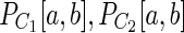) represents a bulge that satisfies weakened relative length difference and relative coverage thresholds. Bulge criterion is considered satisfied if all such checks are successfull. Tail criterion: let be longer than . We check whether there exists a vertex u in and a path Q from p_n to u such that is a prefix of Q and () is a bulge that satisfies the same conditions as in bulge criterion. Tail criterion is considered satisfied if this check and analogous check for p₁ are successful. An example of overlapping pair of paths is shown in Figure 9.

FIG. 9.

Search overlap between two haplocontigs P₁ and P₂ with masked polymorphisms. Longest common subsequence P of PC₁ and PC₂ is highlighted in green. Consecutive vertices of P correspond to either edges of graph or bulges and thus satisfy bulge criterion. Tail criterion is also met: last vertex of P₁ matches with the last vertex of P. First vertex of P₂ lies on a path that forms a bulge with subpath of P₁. Thus, we report that P₁ and P₂ overlap.

9. Appendix D: Dipspades as a Comparative Assembler—Assembling Multiple S. commune Genomes

Below we show that dipSPAdes can be used as a comparative assembler to significantly improve on S. commune assembly and produce contigs with N50 as large as 0.68 Mbp, even from short reads with relatively short insert sizes. First, we assembled S. commune datasets, A8 and B3, separately and obtained high-quality contigs (Table 7). Then we ran dipSPAdes using mixed contigs from computed separate assemblies as haplocontigs. Table 7 shows that the quality of consensus assembly of two S. commune genomes improves on the quality of separate assemblies. As Table 8 shows, both HaploMerger and dipSPAdes show improved results and increase the length of the SPAdes contigs (from N50 82 kbp to N50 386 kbp and 375 kbp). We further extended the described approach to combine five more S. commune libraries: Mi1, B1, FL, A4, and A5 by iteratively mixing previously computed consensus contigs with separate assemblies of S. commune individuals (Table 9). This approach can be generalized to any number of individual genomes that differ from each other by less than 10%. Table 10 shows that assembly of reads from seven different S. commune genomes significantly improves on the assembly of a reference S. commune. Note that the resulting reference assembly does not represent any of the seven S. commune genomes but rather represents a consensus of their genomes.

Table 7.

Separate Assemblies of Two S. commune Libraries, A8 and B3, Using SPAdes and Velvet

	A8		B3
	Velvet	SPAdes	Velvet	SPAdes
Total length (Mbp)	35.37	36.47	35.37	36.53
No. contigs	3886	1893	4472	1804
Largest contig	186960	524070	162349	780644
N50	23509	98988	16744	104280
N75	11217	44666	8656	46746

Table 8.

Joint Assembly of Two S. commune (A8 and B3) Genomes

	HaploMerger	Velvet	SPAdes	dipSPAdes
Expected total length (Mbp)	38.9	77.8	77.8	38.9
Total length (Mbp)	36.00	70.75	73.26	37.99
No. contigs	981	8358	4289	969
Largest contig	1677298	186960	510594	1568684
N50	386031	19416	82552	375236
N75	141045	9707	34743	104312

Haplocontigs in SPAdes were generated as a mixture of contigs from separate assemblies of A8 and B3.

Table 9.

Libraries of S. commune Used in the Consensus Assembly

	Mi1	B1	FL	A4	A5
Total length (Mbp)	36.30	37.00	36.10	36.70	36.70
No. contigs	1795	1838	1974	1928	1998
Largest contig	524292	592920	400383	519910	454167
N50	99854	94872	80125	87625	88650
N75	42380	40825	37159	39017	38977

Table 10.

Assembly of Consensus S. commune Genome from Multiple Libraries

Used libraries	Total length (Mbp)	No. contigs	Largest contig	N50	N75
A8-B3	37.99	969	1568684	375236	104312
A8-B3-Mi1	36.20	500	1568684	454899	214922
A8-B3-Mi1-B1	39.50	440	1568684	551577	258782
A8-B3-Mi1-B1-FL	38.50	488	2113559	552311	229777
A8-B3-Mi1-B1-FL-A4-A5	37.30	289	2113291	680068	351673

10. Appendix E: S. commune Assembly Quality Analysis

We performed additional analysis to check the potential errors in dipSPAdes assemblies. We compared contigs produced by SPAdes on separate (SEP) S. commune datasets, A8 and B3 (Table 7), with the consensus contigs produced by dipSPAdes on mixed (MIX) S. commune datasets (Table 3). Both MIX and SEP contigs represent the S. commune genome. Since SPAdes was previously shown to produce rather accurate assemblies (Bankevich et al., 2012), we assume that SEP contigs are accurate. Further we describe how we detected misassemblies in MIX contigs by matching them against SEP contigs.

We calculated and manually analyzed alignments between SEP and 150 MIX contigs (all contigs of length at least 50 kbp) using MAUVE tool (Darling et al., 2004). We observed three possible types of alignments between MIX and SEP contigs (illustrated in Fig. 10). Since SEP contigs have much higher N50 than MIX contigs (≈100 kbp versus ≈27 kbp, see Tables 3 and 7), most MIX contigs match to segments of SEP contigs (Fig. 10a). We classify such MIX contigs as correctly assembled. Some MIX contigs that match to suffixes and prefixes of SEP contigs (Fig. 10b) do not necessarily represent assembly errors and thus remain unclassified. The third type of alignment represents misassembled MIX contig that aligns to internal segments of two or more SEP contigs (Fig. 10c).

FIG. 10.

(a) MIX contig that fully aligns to a single SEP contig. (b) MIX contig that aligns to the suffix of contig SEP₁ and the prefix of contig SEP₂. (c) A likely assembly error.

This analysis applied to S. commune contigs revealed only one potentially misassembled MIX contig with a single assembly breakpoint. Thus, using unique features of the S. commune datasets, we were able to evaluate the accuracy of contigs in the assembly of an HP genome even without a reference genome.

11. Appendix F. Additional Benchmarking

In order to check dipSPAdes performance in a more realistic setting, we simulated two datasets with medium (5%) and high (10%) polymorphism rates and uneven distribution of SNPs. First we simulated a polymorphic reference genome using one of C. dubliniensis haplomes as a base genome and constructed two Markov models to generate polymorphisms in the base genome. Each MM had two states “low” and “high” corresponding to low and high polymorphism rates, respectively. For the first, MM has the emission probabilities of mismatches, and indels were set to 0.005 for “low” state and 0.06 for “high” state. For the second MM the emission probabilities of mismatches and indels were set to 0.01 for “low” state and 0.12 for “high” state. For both MMs the transition probability from “low” to “high” (“high” to “low”) states were set to 0.01 (0.002). Heterozygous haplomes generated by such MMs yield average polymorphism rates close to 5% and 10%. Thus, DNA sequences emitted by these MMs provide simulations of diploid genomes with 5% and 10% polymorphism level. This simulation resulted in two diploid copies with high rate of SNPs and indels grouped into polymorphic islands separated by conservative regions with low polymorphism rate. We simulated error-free reads in the same way as described in the Results section. Tables 11 and 12 show that dipSPAdes significantly improved on SPAdes contigs and outperformed HaploMerger.

Table 11.

Assembly of Simulated HP Diploid Genome with Moderate Polymorphism Rate (5%) and Uneven SNP Distribution Based on C. dubliniensis Haplome

	Velvet	SPAdes	HaploMerger	dipSPAdes
Expected total length (Mbp)	29.2	29.2	14.6	14.6
Total length (Mbp)	13.91	28.29	14.26	13.73
No. contigs	18136	2506	1146	97
Largest contig	3415	91821	91821	1301944
NA50	765	19823	21288	397065
NA75	612	10897	11821	169301
No. misassemblies	0	0	0	2

Table 12.

Assembly of Simulated HP Diploid Genome with High Polymorphism Rate (10%) and Uneven SNP Distribution Based on C. dubliniensis Haplome

	Velvet	SPAdes	HaploMerger	dipSPAdes
Expected total length (Mbp)	29.2	29.2	14.6	14.6
Total length (Mbp)	24.21	28.79	14.55	14.75
No. contigs	18996	991	392	60
Largest contig	8751	278131	278131	1482039
NA50	1502	57039	65415	777890
NA75	954	33859	38399	389623
No. misassemblies	0	0	1	2

Acknowledgments

We are indebted to Drs. Alexey Kondrashov, Sergey Naumenko, Maria Baranova, and Yegor Bazykin for many helpful discussions. The work of Y.S., A.B., and P.A.P. was supported by the Government of the Russian Federation, grant 11.G34.31.0018. P.A.P. was partially supported by the National Institutes of Health, grant 3P41RR024851-02S1. We would like to thank Dr. Alexey Kondrashev for providing sequencing data of S. commune and A. protococcarum that were generated with support of the Government of the Russian Federation, grant 11.G34.31.0008. We are grateful to Dr. Shengfeng Huang and Dr. Anton Korobeynikov for help with HaploMerger benchmarking. We are also grateful to Dr. Alla Lapidus for help with preparing this article.

Author Disclosure Statement

No competing financial interests exist.

References

- Aguiar D., and Istrail S. 2012. Hapcompass: a fast cycle basis algorithm for accurate haplotype assembly of sequence data. J. Comput. Biol. 19, 577–590 [DOI] [PMC free article] [PubMed] [Google Scholar]
- Aparicio S., Chapman J., Stupka E., et al. 2002. Whole-genome shotgun assembly and analysis of the genome of Fugu rubripes. Science 297, 1301–1310 [DOI] [PubMed] [Google Scholar]
- Bankevich A., Nurk S., Antipov D., et al. 2012. SPAdes: a new genome assembly algorithm and its applications to single-cell sequencing. J. Comput. Biol. 19, 455–477 [DOI] [PMC free article] [PubMed] [Google Scholar]
- Bansal V., Halpern A.L., Axelrod N., et al. 2008. An MCMC algorithm for haplotype assembly from whole-genome sequence data. Genome Res. 18, 1336–1346 [DOI] [PMC free article] [PubMed] [Google Scholar]
- Barriere A., Yang S., Pekarek E., et al. 2009. Detecting heterozygosity in shotgun genome assemblies: lessons from obligately outcrossing nematodes. Genome Res. 19, 470–480 [DOI] [PMC free article] [PubMed] [Google Scholar]
- Batzoglou S., Jaffe D., Stanley K., et al. 2002. ARACHNE: a whole-genome shotgun assembler. Genome Res. 12, 177–189 [DOI] [PMC free article] [PubMed] [Google Scholar]
- Compeau F., Pevzner P., and Tesler G. 2011. How to apply de bruijn graphs to genome assembly. Nat. Biotechnol. 29, 987–991 [DOI] [PMC free article] [PubMed] [Google Scholar]
- Darling A., Mau B., Blattner F., et al. 2004. Mauve: multiple alignment of conserved genomic sequence with rearrangements. Genome Res. 14, 1394–1403 [DOI] [PMC free article] [PubMed] [Google Scholar]
- Dehal P., Satou Y., Campbell R., et al. 2002. The draft genome of Ciona intestinalis: insights into chordate and vertebrate origins. Science 298, 215767. [DOI] [PubMed] [Google Scholar]
- Donmez N., and Brudno M. 2011. Hapsembler: an assembler for highly polymorphic genomes. Research in Computational Molecular Biology—15th Annual International Conference, RECOMB 2011, Vancouver, BC, Canada, March28–31, 2011, LNCS, volume 6577, pp. 38–52 [Google Scholar]
- Gurevich A., Saveliev V., Vyahhi N., et al. 2013. QUAST: quality assessment tool for genome assemblies. Bioinformatics 29, 1072–1075 [DOI] [PMC free article] [PubMed] [Google Scholar]
- He D., Choi A., Pipatsrisawat K., et al. 2010. Optimal algorithms for haplotype assembly from whole-genome sequence data. Bioinformatics 26, i183–i190 [DOI] [PMC free article] [PubMed] [Google Scholar]
- Huang S., Chen Z., Huang G., et al. 2012. HaploMerger: reconstructing allelic relationships for polymorphic diploid genome assemblies. Genome Res. 22, 1581–1588 [DOI] [PMC free article] [PubMed] [Google Scholar]
- Magoc T., Pabinger S., Canzar S., et al. 2013. GAGE-B: An evaluation of genome assemblers for bacterial organiss. Bioinformatics 29, 1718–1725 [DOI] [PMC free article] [PubMed] [Google Scholar]
- Ohm R., de Jong J., Lugones L., et al. 2010. Genome sequence of the model mushroom Schizophyllum commune. Nature 28, 95763. [DOI] [PubMed] [Google Scholar]
- Pevzner P., Tang H., and Waterman M. 2001. An Eulerian path approach to DNA fragment assembly. Proc. Natl. Acad. Sci. USA 98, 9748–9753 [DOI] [PMC free article] [PubMed] [Google Scholar]
- Prjibelski A., Vasilinetc I., Bankevich A., et al. 2014. ExSPAnder: a universal repeat resolver for DNA fragment assembly. Bioinformatics 30, i293–i301 [DOI] [PMC free article] [PubMed] [Google Scholar]
- Safonova Y., Bankevich A., and Pevzner P.A. 2014. Research in Computational Molecular Biology—18th Annual International Conference, RECOMB 2014, Pittsburgh, PA, April2–5, 2014, LNCS, volume 8394, pp. 265–279 [Google Scholar]
- Salzberg S.L., Phillippy A., Zimin A., et al. 2012. GAGE: A critical evaluation of genome assemblies and assembly algorithms. Genome Res. 22, 557–567 [DOI] [PMC free article] [PubMed] [Google Scholar]
- Vinson J.P., Jaffe D.B., O'Neill K., et al. 2005. Assembly of polymorphic genomes: algorithms and application to Ciona savignyi. Genome Res. 15, 1127–1135 [DOI] [PMC free article] [PubMed] [Google Scholar]
- Xie M., Wang J., and Chen J. 2008. A model of higher accuracy for the individual haplotyping problem based on weighted SNP fragments and genotype with errors. Bioinformatics 24, i105–i113 [DOI] [PMC free article] [PubMed] [Google Scholar]
- Zerbino D., and Birney E. 2008. Velvet: algorithms for de novo short read assembly using de Bruijn graphs. Genome Res. 18, 821–829 [DOI] [PMC free article] [PubMed] [Google Scholar]
- Zhao Y.Y., Wu L.Y., Zhang J.H., et al. 2005. Haplotype assembly from aligned weighted SNP fragments. Comput. Biol. Chem. 29, 281–287 [DOI] [PubMed] [Google Scholar]