Reconstructing Breakage Fusion Bridge Architectures Using Noisy Copy Numbers

Abstract

The Breakage Fusion Bridge (BFB) process is a key marker for genomic instability, producing highly rearranged genomes in relatively small numbers of cell cycles. While the process itself was observed during the late 1930s, little is known about the extent of BFB in tumor genome evolution. Moreover, BFB can dramatically increase copy numbers of chromosomal segments, which in turn hardens the tasks of both reference-assisted and ab initio genome assembly. Based on available data such as Next Generation Sequencing (NGS) and Array Comparative Genomic Hybridization (aCGH) data, we show here how BFB evidence may be identified, and how to enumerate all possible evolutions of the process with respect to observed data. Specifically, we describe practical algorithms that, given a chromosomal arm segmentation and noisy segment copy number estimates, produce all segment count vectors supported by the data that can be produced by BFB, and all corresponding BFB architectures. This extends the scope of analyses described in our previous work, which produced a single count vector and architecture per instance. We apply these analyses to a comprehensive human cancer dataset, demonstrate the effectiveness and efficiency of the computation, and suggest methods for further assertions of candidate BFB samples. Source code of our tool can be found online.

1. Introduction

The origin of a tumor cell is marked by genomic instability (Hanahan and Weinberg, 2011). Spontaneous, viral, or other kinds of mechanisms may cause genomic segment deletions, duplications, translocations, inversions, etc., producing rearranged genomes with a possibly malignant nature. Thus, decoding mechanisms that generate rearranged genomes is critical to understanding cancer. Numerous mechanisms were proposed, including the faulty repair of double-stranded DNA breaks by recombination or end-joining and polymerase hopping caused by replication fork collapse (Carr et al., 2011; Hastings et al., 2009). These mechanisms are generally not directly observable, so their elucidation requires the deciphering of often subtle clues after genomic instability has ceased. An important source of information in this respect is the architecture of the rearranged genome, that is, the description of its chromosomes in terms of concatenations of segments from the original genome.

Breakage Fusion Bridge (BFB) is one model of a genome rearrangement process, which was first proposed by Barbara McClintock in the 1930s (McClintock, 1938, 1941). Recently, it has seen renewed interest as a possible mechanism in tumor genome evolution (Bignell et al., 2007; Campbell et al., 2010; Greenman et al., 2012). BFB begins with a telomeric loss on a chromosome, including a loss of a sequential pattern that signals the location of chromosome termination. During cell division the telomere-lacking chromosome replicates, and its two sister chromatids fuse together (possibly due to some DNA repair mechanism falsely induced by the cell). This fusion produces a dicentric chromosome of palindromic structure, which is later torn apart at some random point as the centromeres of the dicentric chromosome migrate to opposite poles of the cell. One part of the torn chromosome includes the fusion region and some tandemly inverted chromosomal suffix duplication, and the other part lacks the corresponding suffix. The two daughter cells receive these rearranged chromosomes, both are missing the telomeric region, and the cycle can repeat (Fig. 1).

FIG. 1.

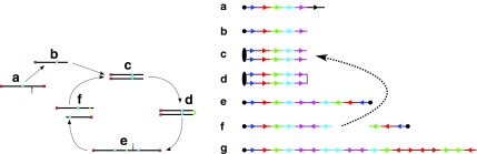
The BFB process. To the left, the different stages of a BFB cycle are presented. To the right, corresponding modifications over an exemplary chromosomal arm are shown. (a) A normal chromosome. (b) The chromosome loses its telomere. (c) The chromosome is duplicated during cell division. (d) Sister chromatids are fused together. (e) Centromeres migrate to opposite poles of the cell. (f) The fused chromosome is torn apart at some random position between the two centromeres, causing one copy to have an inverted suffix duplication, while the other copy has a trimmed suffix. Both copies lack a telomere and therefore may undergo additional BFB cycles. (g) After several BFB cycles, the chromosome architecture exhibits significant increases in segment copy numbers, as well as fold-back patterns.

In contrast to other mechanisms, BFB can actually be observed in progress using methods that have been available for decades (McClintock, 1941). Cytogenetic techniques can reveal the anaphase bridges, dicentric chromosomes, and homogeneously staining regions that have long been the canonical evidence for BFB. However, these techniques are useful only in cases where the BFB cycles are ongoing. While useful in understanding the mechanism, they do not address the question of whether BFB occurs extensively in evolving tumor genomes.

Recently, researchers (including us) have started looking at modern available data in order to demonstrate BFB occurrence after the process has ceased, including Fluorescent In Situ Hybridization (FISH), Array Comparative Genomic Hybridization (aCGH), and Next Generation Sequencing (NGS) data. These methods take advantage of distinctive BFB features exposed by such data, including the abundance of fold-back inversions (i.e., duplicated chromosomal segments arranged in a head-to-head orientation (Bignell et al., 2007; Campbell et al., 2010), patterns of interleaving segments of alternating orientations (Kitada and Yamasaki, 2008; Reshmi et al., 2007), and combinatorial properties of segment counts when copy number variations are due to BFB (Kinsella and Bafna, 2012; Zakov et al., 2013). In fact, if the architecture of the rearranged genome is known, it is possible to decide if this architecture can be produced by BFB (Kinsella and Bafna, 2012). Properties of the space of different BFB evolutions are explored in Greenman et al. (2012).

Partial knowledge regarding the architecture can be revealed by FISH analyses (Kitada and Yamasaki, 2008), which uses fluorescence markers to identify the physical locations of predetermined sequences on the rearranged genome. However, such experiments are relatively expensive and can only be performed in a small number of cases. A more common measurement is NGS data, which contain a big set of short sequenced reads extracted from a donor genome. Such data is typically used for predicting the entire donor genomic sequence by computationally assembling the reads, sometimes facilitated by consulting a similar presequenced reference genome. Unfortunately, BFB and other mechanisms can produce massively rearranged and highly repetitive genomes. This complicates the task of assembly-based sequencing due to the multiple ambiguous manners the repetitive reads may be assembled, and the lack of a relevant reference template. Nevertheless, NGS data can still be analyzed in order to infer some indirect information regarding the donor genome architecture (Alkan et al., 2009; Chiang et al., 2009; Medvedev et al., 2009; Yoon et al., 2009). After aligning the reads against a reference genome, their genomic location distribution can be used in order to identify segments on the reference genome of coherent read coverage, and to estimate the number of times each such segment repeats in the donor genome. We will refer to the output of the latter kind of analysis as copy number data. Other methods to obtain copy number data are based on analyzing aCGH data (Eckel-Passow et al., 2011; Greenman et al., 2010; Olshen et al., 2004; Venkatraman and Olshen, 2007) (Fig. 2). Due to the noisy nature of both NGS and aCGH data, count estimates may be inaccurate, and the true segment count is likely to fall within some interval of integers around the estimated value. We use the term noisy copy number data when referring to information regarding such intervals of possible count values. In addition to copy number data, NGS data can be used in order to produce contigs (chromosomal segments that may be assembled unambiguously), and aberrant segment adjacencies can be exposed by discordant reads, restricting the set of possible contig-based architectures.

FIG. 2.

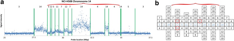
(a) aCGH data for a part of the q-arm of human chromosome 14 in the NCI-H508 cell line. Each data point corresponds to a probe on the array, where its x-coordinate gives the probe's sequence chromosomal position, and y-coordinate gives its measured intensity (log-ratio). The data points are clustered into segments, and an estimated segment copy number appears above each segment. (b) A visualization of the corresponding noisy copy number data. Estimated counts appear in light blue, and the column around each count represents possible deviations from the estimation. The region under the red curly bracket reflects a BFB candidate. Its corresponding estimated counts are [5, 12, 5, 11, 7, 12, 7, 14, 4, 14, 4], which under minor modifications yield the two BFB vectors [5, 13, 5, 11, 7, 12, 8, 14, 4, 14, 4] or [5, 11, 5, 11, 7, 12, 8, 14, 4, 14, 4]. Data is taken from Bignell et al. (2010) [segmentation and copy number analysis were computed using the PICNIC software (Greenman et al., 2010)].

In previous work (Kinsella and Bafna, 2012; Zakov et al., 2013), we showed how to analyze noisy copy number data in order to decide if it is likely to observe the input data under the assumption that the underlying rearrangement process is BFB. Specifically, we designed algorithms that produce a single BFB architecture over the given segments in which segment counts are supported by the data, if such an architecture exists. We applied these algorithms in order to analyze a comprehensive aCGH dataset of cancer cell lines (Bignell et al., 2010), as well as sequence data from primary tumors (Campbell et al., 2010), and identified a small subset of candidate samples exhibiting BFB hallmarks. Here, we extend the scope of the analysis and describe algorithms that report all count settings supported by the data, which can be explained by BFB, and all corresponding BFB architectures. Although the theoretical time bounds for these new algorithms may be exponential, we show that in practice they are efficient and apply an informed search (Pearl, 1984) optimization that further improves their practical efficiency.

Therefore, our proposed algorithms satisfy an important need. While our work postulates the existence of BFB using statistical arguments, additional physical assertions can be obtained with FISH and aberrant read analyses. Starting with noisy copy number data, our tool can be used to enumerate all possible BFB architectures. These candidate architectures can then be used toward a small set of FISH experiments (with a limited number of fluorescence markers) to validate and refine the predicted genomic architecture.

2. Problem Definition

Computational BFB-related problems were previously formulated in Kinsella and Bafna (2012) and Zakov et al. (2013). For completeness, we give here the main definitions from these works and formulate new problems first addressed here.

A DNA segment σ is a string over the DNA nucleotide alphabet A, C, G, T. The reversed segment of a segment σ, denoted here by , is the string obtained by reading σ backwards and replacing each nucleotide with its complementary nucleotide (A ↔ T, C ↔ G). For example, the reverse of a segment σ = CGGAT is the segment . In the rest of this article, it is assumed we operate on a given chromosomal arm with a fixed segmentation and denote its list of k segments by , ordered from the centromeric segment σ₁ to the telomeric segment σ_k. The term “string” refers to a genomic architecture over these segments, that is, a concatenation of segments from Σ and their reversed forms. Greek letters α, β, γ, and ρ denote strings, and bar notation indicates reversed strings. For example, if . An empty string is denoted by ɛ. The notation α_l,t represents the continuous chromosomal region , where α_l,t = ɛ when t < l. To facilitate reading, are replaced by in concrete examples.

A BFB cycle applied over a chromosomal arm can be viewed as a special rearrangement procedure, in which some telomeric suffix of the arm is duplicated, inverted, and concatenated tandemly at the telomeric end of the arm. A string β can be derived from a string α via a BFB process if it is possible to apply a series of zero or more BFB cycles over α and obtain β (Fig. 3a). This notion is formally captured by the following definition.

FIG. 3.

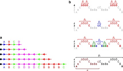
(a) A BFB process generating a string α: . (b) The layers of the BFB palindrome . The block collections are B⁴ = {4β₁}, B³ = {2β₂, β₃}, B² = {2β₄, β₅, 2β₆}, and B¹ = {β₇}.

Definition 1 For two strings α, β, say that if α = β, or there are some strings ρ, γ such that γ ≠ ɛ, α = ργ, and . Say that α is an l-BFB string if for some t, and say that α is a BFB string if it is an l-BFB string for some l.

It is worth mentioning that in reality a BFB cycle can also delete a suffix of a chromosome in case we consider the trimmed chromosomal arm. It is simple to show that for any BFB process that contains such suffix-trimming cycles there is an equivalent process in which only elongation cycles occur (Kinsella and Bafna, 2012). For example, the BFB string obtained by the process can also be obtained by the process . Thus, we can assume without loss of generality that all BFB cycles are of the form of a tandem suffix duplication.

By definition ɛ = α_l,l−1 is an l-BFB string for every l ≥ 1. For a nonempty string α, define top(α) = max {t : σ_t appears in α} and define top(ɛ) = 0. It is simple to observe that when α is an l-BFB string, it must start with the prefix α_l,t for t = top(α), since BFB cycles can only duplicate previously appearing letters and never generate new ones.

The count vector of a string α is a vector of integers, where for every 1 ≤ l ≤ k, n_l is the total number of occurrences of σ_l and in α. For example, for . Say that a vector is a BFB vector if there exists some BFB string α such that . In the previous example is a BFB vector due to the BFB process .

The computational analyses presented in this article aim to detect evidence for BFB, given a preanalyzed segmentation of the genome and corresponding copy number data. We assume that noisy copy number data is represented by a weight function , where w_l,n is a nonnegative weight associated with the copy number n for the l-th segment. It may be assumed w.l.o.g. that all weights w_l,n satisfy 0 ≤ w_l,n ≤ 1. The weight of a count vector is given by , and by assumption . In some cases, we refer to prefixes and suffixes of , which may be empty if l = 1 or l = k + 1, respectively. Define the weights of such subvectors accordingly, that is, and , where the weight of an empty vector is 1 by definition. Thus, for every .

If some data analysis produces segment count probabilities Pr (n_l = n) for every segment σ_l and every count , weights can be set to these probabilities choosing w_l,n = Pr (n_l = n). This way, the weight of a count vector is the probability this vector reflects the true segment counts given the observed data. Another way to set weights given such probabilities would be to choose weights by setting , where is the most likely count for the l-th segment. Here, the weight of a count vector gives the ratio between its probability and the probability of a most likely vector. Nevertheless weights are more general than probabilities and can be used as a heuristic count error modeling even when no probabilistic model is available.

In Zakov et al. (2013), several variants of BFB problems were formulated. Below we restate these problems and add two new variants addressed in the current work:

BFB problem variants

Input: A count vector , or a weight function W and a minimum weight threshold 0 < η ≤ 1.

• 1. The decision variant (Zakov et al., 2013): given , decide if is a BFB vector.

• 2. The string search variant (Zakov et al., 2013): if is a BFB vector, find a BFB string α such that .

• 3. The vector search variant (denoted the distance variant in Zakov et al., 2013): given W and η, report a maximum weight BFB vector in case there exists such a vector with , and otherwise report “FAILED.”

• 4. The exhaustive vector search variant: given W and η, report all BFB vectors with .

• 5. The exhaustive string search variant: given W and η, report all BFB strings α such that .

For a count vector , define and . Note that is the total length of a string admitting , and is proportional to the number of bits needed for representing . For a weight function W and a weight η, define , and . In Zakov et al. (2013), it was shown that the BFB decision variant can be solved using bit operations (i.e., linear time in the input length), the string search variant can be solved in operations (i.e., linear time in the output length), and that the vector search variant can be solved using at most a subexponential number of operations 2^{O(log2 N(W,η))}. Here, we give algorithms for the two new exhaustive search variants. While theoretically the output of these algorithms can be exponential with respect to N(W, η), we show that for realistic inputs this output is manageable. In addition, we describe an Informed Search (IS) approach that significantly reduces the running time in practice by eliminating irrelevant search paths and traversing only paths that are guaranteed to produce valid solutions.

3. Algorithms

In this section we develop algorithms for the two exhaustive search variants of the BFB problem. Next, we describe some ideas taken from Zakov et al. (2013), upon which the algorithms presented here are built.

3.1. Notation and previous results

An l-BFB palindrome is an l-BFB string of the form . It can be shown that is an l-BFB palindrome if and only if α is an l-BFB string. By definition, is an l-BFB palindrome for every l ≥ 1. In addition, observe that when we have that . This allows replacing the question “is there a BFB string admitting the count vector ” by the equivalent question “is there a BFB palindrome admitting the count vector ”.

An l-block is a string of the form , where β′ is an (l +1)-BFB palindrome. It can be shown that an l-block is a special form of an l-BFB palindrome, and that every l-BFB palindrome is some palindromic concatenation of l-blocks. Nevertheless, not every palindromic concatenation of l-blocks yields a valid l-BFB palindrome. For example, two copies of the 2-block and one copy of the block can be concatenated to form the 2-BFB palindrome . The validity of this palindrome can be asserted from the process . On the other hand, the only palindromic concatenation of one copy of and two copies of is the string . This string is not a valid BFB string, since a BFB string over the letters {B, C} must start with the prefix α_2,3 = BC. Claim 1 in Zakov et al. (2013), recited here in the Appendix, gives a required and sufficient condition for block concatenations that form valid BFB palindromes.

The idea of decomposing BFB palindromes into blocks allows us to adopt a layeresd view of BFB palindromes, as follows (Fig. 3). Let be a 1-BFB palindrome, where . As claimed above, β is a palindromic concatenation of 1-blocks. Denote by B¹ the collection of all 1-blocks whose concatenation forms β. Every 1-block in B¹ is a string of the form , where β′ is some 2-BFB palindrome. As there are 2n₁ occurrences of A and in β, and each block in B¹ contains exactly two such occurrences, the total number of blocks in B¹ is exactly n₁. Masking the letters A and from all blocks in B¹, the collection becomes a 2-BFB palindrome collection of size n₁. The 2-BFB palindromes in this collection can be further decomposed into two-blocks, yielding a collection B² of two-blocks. Similarly as above, B² contains exactly n₂ blocks. This process can continue inductively, yielding for every 1 ≤ l ≤ k a corresponding collection B^l of l-blocks, whose size is n_l. One may also imagine an additional collection in this series B^k+1, containing zero (k + 1)-blocks.

This layered view is exploited in a reversed order by the algorithms in Zakov et al. (2013), developing a BFB palindrome given an input count vector : Starting with an empty collection B^k+1 of (k + 1)-blocks, the algorithm computes iteratively a sequence of collections , each collection B^l is an l-block collection of size n_l. In order to generate B^l, the algorithm first concatenates (l + 1)-blocks from B^l+1, forming a collection B of (l + 1)-BFB palindromes of size n_l (this procedure is called folding). Then, each (l + 1)-BFB palindrome β′ ∈ B is wrapped with a pair of σ_l segments, rendering it into an l-block , and B^l is set to be the collection containing all these l-blocks. The final collection of 1-blocks B¹ is folded one more time into a single 1-BFB palindrome , and the algorithm returns the half-length prefix α of this palindrome as a BFB string admitting the input count vector .

Figure 3b illustrates a possible run of the algorithm over the input count vector . First, the algorithm initializes an empty collection of blocks B⁵. In the first iteration, there is a need to perform concatenations of blocks in B⁵ and produce n₄ = 4 BFB palindromes. Such palindromes may only be obtained by concatenating zero elements (as there are no elements in B⁵), and so four empty strings are generated in this folding process, yielding the BFB palindrome collection {4ɛ}. Next, each palindrome in this collection is wrapped by σ₄ = D and , producing the collection of blocks . In the next iteration, the collection B⁴ needs to reduce its size from n₄ = 4 into n₃ = 3 by concatenating its elements to produce BFB palindromes. In this example, there are two concatenations of two elements the form β₁β₁, and one concatenation of zero elements that produces an empty string ɛ. The BFB palindromes in the resulting folded collection {2β₁β₁, ɛ}, are wrapped by σ₃ = C and , yielding the block collection . This process continues for two more iterations, generating similarly the collections B² = {2β₄, β₅, 2β₆} and B¹ = {β7}. All elements in the last collection B¹ are then concatenated into a single BFB palindrome β (in this example B¹ contains a single element β₇, and so β = β₇), and the returned string α is the half-length prefix of this palindrome.

The ability of the schematic algorithm above to process the entire input vector and produce a corresponding BFB string depends on its ability to fold intermediate collections B^l computed along its run. In cases where it cannot fold some intermediate block collection, it returns a fail message, implying no BFB string admits the input vector .

A case where folding cannot be applied is, for example, the case where n₂ = 2, , and n₁ = 1. In this case, since both possible concatenations and of the two elements in B² are non-palindromic, the folding procedure must fail at this stage. Another example of a fail folding is the case where n₂ = 3, , and n₁ = 1. In this case, though there exists a palindromic concatenation of all three elements in B², this concatenation is not a valid BFB palindrome (see example above), and so the collection may not be folded.

In Zakov et al. (2013), it was shown that the ability to fold a block collection depends on a property called the signature of the collection. A signature of an l-BFB palindrome collection B is an infinite sequence of integers with the following properties: (1) the first nonzero element in (if there is such an element) must be positive, (2) the cardinality of , defined by (where abs(s_d) is the absolute value of s_d), equals the size of B, and (3) the values s_d depend only in multiplicities of distinct elements in B and their top values. The prefix of a signature up to its d-th element is denoted by . The formal definition of a signature is given in the Appendix, and we refer intrigued readers to Zakov et al. (2013) for an elaborated discussion on its properties.

We will use the notation to imply that the remaining signature elements after position d are all zeros. From property (2), it follows that for a signature such that , all signature elements s_d for d > log n are zeros, thus signatures can be explicitly represented by a relatively small number of nonzero elements. In particular, from properties (1) and (2) it follows that the only signature of an empty collection is , and that the only signature of a collection containing a single element is . Otherwise, two collections of the same size may have different signatures. From property (3), wrapping an l-BFB palindrome collection (i.e., replacing each l-BFB palindrome β in the collection with an (l − 1)-block ) does not affect its signature.

Signatures can be ranked according to their lexicographic order. That is, say that if there exists an index d such that and , and say that if or . Lemma 2 below implies that the signature series corresponding to the block collections series in a layered representation of a BFB palindrome is lexicographically nondecreasing.

Lemma 2 Let B be an l-block collection with a signature . For any folding B′ of B and its corresponding signature . In addition, for any signature such that (1) and (2) is the lexicographically minimal signature among all signatures of cardinality that meet (1), there exists a folding B′ of B whose signature is .

The proof of Lemma 2 follows from Claims 14 and 28 in Zakov et al. (2013) (Supporting Information). The signatures corresponding to the four block collections in Figure 3b are , and , respectively. Observe that the cardinality of each signature equals the size of the corresponding collection (i.e., the corresponding count in ), and that for every 1 ≤ l < 4.

3.2. Valid signature series

Definition 3 A valid signature series for a vector is a series of lexicographically nonincreasing signatures , satisfying for every , and .

For convenience, we will sometimes consider the signatures and as fixed sentinel additions at the beginning and ending of a valid signature series and mark them respectively by and . If is a BFB count vector, there exists a BFB palindrome β with , and a corresponding collection series in the layers representation of β. Lemma 2 implies that the corresponding signature series for this collection series is a valid signature series for , since for every 0 ≤ l ≤ k, B^l is obtained by applying a folding operation over B^l+1 that can only increase the lexicographic signature rank, and a wrapping operation that does not change the signature. On the other hand, if there exists a valid signature series for , it is possible to generate a BFB palindrome β with as follows. Run the schematic layered algorithm described above with respect to , where each time a folding operation is applied it is such that yields the minimal signature increment with respect to its input and output collections. Since and , Lemma 2 implies that it is possible to fold B^k+1 into a (k + 1)-BFB palindrome collection of size n_k, and that the lexicographically minimal signature of such a collection satisfies . Inductively, each generated block collection B^l in this process has a corresponding signature that satisfies , and from Lemma 2 it can be folded into the next collection in the series B^l−1 without a folding failure. We hence get the following conclusion:

Conclusion 4 A vector is a BFB vector if and only if it has a valid signature series. Moreover, any subsequence of a BFB vector is also a BFB vector, evident by the corresponding subseries of a valid signature series for the full vector.

For example, the vector is a BFB vector, due to the valid signature series . A corresponding BFB string may be obtained by . An example for a vector that does not have a valid signature series is the vector . The only signatures with cardinality 4 that rank lexicographically between and are the signatures and , and the only such signature with cardinality 3 is . The latter signature does not precede lexicographically any of the two possible 4-cardinality signatures, therefore no valid signature series for exists.

A valid signature series for a given count vector, if exists, can be computed iteratively by processing the counts in the vector one by one. This process can be done either by traversing the counts from n₁ to n_k, or traversing them in a reversed order. Next, we describe this computation.

Let be a BFB vector, and let 1 ≤ l ≤ k + 1. Define the right-maximal signature of the prefix of to be if l = 1, and otherwise to be the lexicographically maximal signature in some valid signature series for . Similarly, define the left-minimal signature of the suffix of to be if l = k + 1, and otherwise to be the lexicographically minimal signature in some valid signature series for .

Lemma 5 Let be a BFB vector. For every 1 ≤ l′ ≤ l ≤ k + 1, , and .

Proof: We start by showing the first inequality in the lemma. If l = 1 or follows immediately. Otherwise, consider a valid signature series for . Note that its prefix is a valid signature series for , and its suffix is a valid signature series for . Thus, by definition, .

To show the second inequality in the lemma, let be a valid signature series for such that . Observe similarly as above that . The last inequality in the lemma is shown symmetrically.   ■

The MIN-DECREMENT procedure (Algorithm 1) gets as an input a signature and an integer n ≥ 0, and returns the lexicographically maximal signature such that and if such a signature exists, and otherwise it returns a fail message. Here, for an integer m ≠ 0, the notation d_m represents the maximum integer such that m divides by . Thus, for example, , and . The correctness of this computation is shown in the Appendix. Symmetrically, the MIN-INCREMENT procedure gets as an input a signature and an integer n ≥ 0, and returns the lexicographically minimal signature such that and if such a signature exists, and otherwise it returns a fail message. The pseudocode for this procedure is given in the Appendix, and its proof is symmetric to that of the MIN-DECREMENT procedure.

Lemma 6 If is a BFB vector, , and MIN-DECREMENT() does not fail and returns a signature , then is the right-maximal signature for the BFB vector . Symmetrically, if is a BFB vector, , and MIN-INCREMENT() does not fail and returns a signature , then is the left-minimal signature for the BFB vector .

Proof: We show the first part of the lemma, where the second part is shown symmetrically. First, note that the constructed vector is indeed a BFB vector, due to the corresponding valid signature series obtained by adding to a valid signature series for whose last signature is . Note that . From Lemma 5 , and since it follows that . From the maximality of .  ■

Lemma 6 implies a simple algorithm for deciding if a given vector is a BFB vector. Such an algorithm tries generating a valid signature series for either by starting from the first signature , and generating each signature by applying the MIN-INCREMENT procedure with respect to and n_l, or by starting from the last signature , and generating each signature by applying the MIN-DECREMENT procedure with respect to and n_l. If the MIN-INCREMENT or MIN-DECREMENT procedures fail at some stage, then the algorithm reports not to be a BFB vector. Otherwise, the algorithm succeeds to generate a valid signature series for , and reports to be a BFB vector. As a matter of fact, Algorithm DECISION-BFB in Zakov et al. (2013) is equivalent to the right-to-left version of the above algorithm.

3.3. Solving the exhaustive BFB variants

In this section, let W be a weight function, and 0 < η ≤ 1 some weight threshold. Let 0 ≤ l ≤ k, and consider the set of all signature-weight pairs of the form such that is a BFB vector and . Say that the pair within this set dominates the pair if and w′≤w. Define the l-th boundary curve C^l with respect to W and η as the maximal subset of these pairs satisfying that no pair in C^l dominates another pair in C^l, and note that C^l is unique. Traversing the pairs in C^l from lowest to highest lexicographic signature rank, the series of signature values strictly increases, while the series of weight values strictly decreases, yielding a steplike curve (Fig. 4). Given W and η, Algorithm 2 generates boundary curves C^l for every 0 ≤ l ≤ k, which will later be exploited by algorithms for the BFB exhaustive vector and string search variants.

FIG. 4.

A boundary curve. Points correspond to pairs of the form , with x-coordinate reflecting the lexicographic rank of , and y-coordinate equaling w. Blue points belong to the boundary curve, and green points are dominated by points on the curve.

Proof: [Algorithm 2] Note that a pair in C⁰ corresponds to a right-maximal signature and a weight of an empty vector. By definition, the only such pair is the pair , and the algorithm correctly sets C⁰ to contain this single pair (line 1). Now, assuming inductively the algorithm has computed correctly the curve C^l−1, we prove it also computes correctly C^l. It is clear from lines 6 and 7 of the algorithm that no pair in the set C^l computed by the algorithm dominates another pair in this set. It therefore remains to show that after the l-th loop iteration was executed: (1) for every BFB vector with there exists a pair , which dominates , and (2) for every pair there exists some BFB vector such that and .

We start by showing (1). Let be a BFB vector with , and consider its prefix . Observe that . As is also a BFB vector, the inductive assumption implies that C^l−1 contains a pair that dominates . From Lemma 5, . Since , running MIN-DECREMENT does not fail, and returns a signature such that and . As , it follows that the algorithm runs the code in lines 5–7 with respect to n_l and . In particular, the algorithm updates C^l with the pair for (lines 6–7). Therefore, at the end of the l-th iteration, either C^l contains , or it contains some other signature-weight pair that dominates , and so it contains a pair that dominates .

To show (2), assume that C^l contains a pair . This pair was added to C^l in line 7 of the algorithm, which means there exists some pair such that for , and . From the inductive assumption, there is BFB vector such that and . For the vector , lemma 6 implies that . In addition, , and the lemma follows.   ■

In Appendix section 6.2 we show that the number a_n of all signatures with cardinality n satisfies . Since no two pairs in a boundary curve share the same signature, the number of pairs in a boundary curve with cardinality n is bounded by . It would be quite realistic to assume that for a segment l and its corresponding most likely count , all counts n such that w_l,n ≥ η satisfy for some constant x. This implies that the total number of different elements in a boundary curve is bounded by the subexponential term . In particular, the number of candidates examined in line 4 of Algorithm 2 is . Over each such candidate, the condition in line 6 is examined, and it may induce at most one insertion of a pair into C^l, and possibly one future deletion from C^l (if the inserted pair is dominated by a pair that is inserted into C^l later on). It is possible to maintain the pairs in C^l sorted, and implement the condition check in line 6 and insertions and deletions from C^l in line 7 in time per operation, for example, using a self-balancing binary search tree (Knuth, 1998). Thus, the l-th iteration of the algorithm runs in time, and the total running time of the algorithm is .

Next, we present Algorithm 3 for the BFB exhaustive vector search variant. The algorithm processes the segments of the input one by one, starting from the k-th segment down to the first segment. The notation [] is used for denoting a vector whose first element is the integer n, and its remaining suffix is the vector .

Proof: [Algorithm 3] By definition, if the boundary curve C^k is empty, it implies there is no BFB vector with . In this case, the algorithm correctly reports there is no solution to the input (line 1).

Otherwise, we show for every 1 ≤ l ≤ k+1 that the following invariant holds: After Q^l is fully computed, Q^l contains if and only if is a suffix of some BFB vector of weight . In particular, this invariant proves that the returned value Q¹ (line 9) is indeed the solution for the BFB exhaustive vector search variant, and so it only remains to establish the correctness of the invariant.

For l = k + 1, the fact that Q^k+1 contains a single empty suffix (line 2) derives the invariant in a straightforward manner. Otherwise, assuming inductively the invariant holds with respect to Q^l+1, we prove it also holds with respect to Q^l.

Let be a BFB vector of weight , and consider its two suffixes and . From the inductive assumption, . From Lemma 6, satisfies that . Since , the condition in line 5 holds, and lines 6–8 are executed with respect to and . Note that the prefix of is a BFB vector with . From the definition of C^l−1, there exists a pair that dominates the pair . From Lemma 5, . In addition, , and so the condition in line 7 holds, and the algorithm adds into Q^l in line 8.

For the other direction of the invariant, let . Due to the manner it was constructed (lines 5–6), its suffix is in Q^l+1, and from Lemma 6, is a BFB vector with . From line 7, there exists a pair such that and , and so from the definition of C^l−1 there exists a BFB vector for which and . The concatenation of and gives the vector , whose weight satisfies . In addition, is a BFB vector, due to the corresponding valid signature series obtained by concatenating a valid signature series for that ends with and a valid signature series for that starts with , concluding this direction of the proof.   ■

Finally, we describe an algorithm for the exhaustive BFB string search variant. This algorithm applies a similar approach to the exhaustive vector search algorithm in order to produce all BFB strings whose count vector weights are at least η. The pseudocode for this computation is given in Algorithm 4. It starts by generating signature curves exactly as done by Algorithm 3. Then, in each iteration l, instead of computing a set Q^l of count vectors, the algorithm computes a set P^l of l-block collections. The initial collection P^k+1 contains a single empty (k + 1)-block collection. In the l-th iteration, for each (l + 1)-block collection B^l+1 ∈ P^l+1, all possible foldings of B^l+1 are enumerated, and each such folding is rendered into an l-block collection B^l as described in section 3.1 (the term “wrapped folding” in line 5 of the algorithm refers to these l-block collections). The notation W (B^l) is used for denoting the weight of the vector such that is the summation of count vectors of all strings in B^l. The signature and weight of B^l are examined against C^l−1 similarly as done in line 7 of Algorithm 3, and if meeting the condition B^l is added into P^l. After P¹ is computed, all foldings of collections B¹ in P¹ into 1-BFB palindromes are enumerated, and all half-length prefixes of such palindromes are reported. Algorithm 4 can be proven similarly to Algorithm 3, using the following invariant: At the end of the l-th iteration, P^l contains all l-block collections B^l such that there exists some 1-BFB palindrome β in which the l-th layer's block collection is B^l, and the weight of the vector such that satisfies .

4. Results

In order to test our algorithms we have used cancer data taken from the Cancer Genome Project dataset (Bignell et al., 2010). This data covers aCGH samples (Affymetrix Genome-Wide Human SNP Array 6.0) from 746 human cancer cell lines. Segmentation and segment copy numbers are as reported by Bignell et al. (2010), who used the PICNIC software (Greenman et al., 2010) for this analysis. In total, the dataset contains about 35,000 chromosomal arms (746 samples, 23 or 24 chromosomes per sample, 2 arms per chromosome), each arm is segmented, and each segment is assigned an estimated copy number based on the observed aCGH data. As shown in Zakov et al. (2013), short BFB-like count vectors have a high probability to emerge even when the genome was rearranged with mechanisms different from BFB. Thus, in order to detect significant BFB evidence we have filtered the set of chromosomal arms to include only arms with at least eight consecutive segments such that no adjacent segments share the same copy number estimation. After this filtration, the remaining subset included 6589 chromosomal arms. As the estimated counts reflect the expected segment copy numbers in all copies of the chromosome in the sample, we have corrected the counts by reducing p − 1 from each count, where p is the ploidy (i.e., the number of copies) of the chromosome in the sample. Typically p = 2, but since these are heavily rearranged cancer genomes, chromosomal losses and whole chromosomal duplications are not rare. We therefore allowed the value of p to vary between 1 and 5, and run the BFB analyses for each value.

As currently no analysis tool available produces count weights, we have derived such weights from the expected counts reported by PICNIC (after correcting for ploidy). Specifically, for a segment whose observed count is n, the weight of a count n′ was defined by , where is the probability to observe the value x for a random variable distributing according to the Poisson distribution with parameter λ. For each of the obtained weight functions, we used the DISTANCE-BFB algorithm from Zakov et al. (2013) to report all longest BFB subvectors with weight at least η = 0.7. Out of the 6589 samples, 54 samples had for at least one ploidy value 1 ≤ p ≤ 5 a BFB subvector of length at least 8. Some samples had long BFB subvectors with respect to more than one ploidy value, and the total number of obtained BFB vectors was 86.

Then, we considered the segment coordinates and weight functions corresponding to the obtained subvectors and ran Algorithm 3 in order to find all BFB vectors of weights at least η = 0.7 with respect to these weight functions. For these 86 instances, a total number of 19154 heavy BFB vectors were found, with an average of 222 solutions per instance. This reveals an interesting property of the problem when applied over this data: the vast majority of samples, 6535 out of 6589, cannot be explained by any BFB count vector (and thus are unlikely to be obtained from BFB), yet each one of those 54 samples that can be explained by BFB has about several tens or hundreds of corresponding count vectors.

The above analysis was run by two variants of our algorithm—the IS variant described by Algorithm 3, and a variant that runs a similar procedure without applying the IS optimization (essentially, it runs the same code as Algorithm 3, with the exceptions that it does not generate the boundary curves in line 1 and does not apply the condition in line 7 before adding new elements to collections Q^l). The disadvantage of the non-IS variant is in that sets of the form Q^l maintains BFB vectors , which may not be suffixes of some BFB vectors of weight at least η. To measure the gain of the IS algorithm, we count the number of signature increment attempts the algorithms perform (line 5). On average, the IS variant performed 57-fold less increments, with a total number of 5672346 increment attempts over all 86 vectors, versus 325343441 for the non-IS algorithm. While the IS variant has a clear efficiency advantage over the non-IS variant, this advantage might be considered more modest than expected. A possible reason for that is that maximum copy number values reported in Bignell et al. (2010) were limited to 14, even when the data suggests higher copy numbers. In general, higher copy numbers usually imply a higher number of alternative heavy counts, which in turn induce a higher number of possible heavy count vectors. For example, when comparing the two algorithms over the synthetic count vector  = [3, 8, 111, 8, 5, 150, 11, 170, 4, 53, 100, 75, 49, 10, 42, 18], using the same Poisson-based weights as described above and requiring that output vectors weigh at least η = 0.85, the non-IS algorithm runs 218 seconds¹ and performs over 20 million signature increments, whereas the IS algorithm runs 120 milliseconds and performs 635 signature increments. Both algorithms return exactly the same output—a set of 18 BFB vectors. Other simulated inputs can cause memory explosion for the non-IS variant, while being handled efficiently by the IS variant.

5. Discussion and Conclusions

The problem of detecting breakage fusion bridge is challenging, but significant progress has been made in the last few years. Our work suggests that while rare, BFB does occur in tumor-derived cell lines and also in primary tumors. In this work, we describe algorithms that can be used to enumerate all possible BFB architectures given uncertain copy number data.

The results of our analyses heavily depend on the input weights, which in turn depend on separated analyses applied to biological data. While we used here a simple Poisson-based model in order to render fixed available count estimations into weight functions, it is clear that more realistic weighing can be applied. Examining Figure 2, for example, one can observe that different segments demonstrate different variance in signal intensities, implying that some count estimates are more reliable than others. Incorporating segment lengths and signal variance information when choosing count weights is likely to produce more meaningful weights and improve the quality of the analyses output.

Different measurements can yield other types of BFB evidence. For example, deep sequencing experiments can sequence reads spanning genomic breakpoints. In a BFB modified genome, it is expected that many of these breakpoints reflect fold-back inversions (i.e., concatenations between reference segments and their inverted form), while such fold-back patterns are less common in other rearrangement mechanisms (Campbell et al., 2010). Thus, identification of high or low fold-back pattern frequencies can support or weaken the conjecture BFB has occurred, respectively. Such evidence is less frequent in currently available data, as reliable breakpoint information requires sequencing to a relatively high depth of coverage (while copy number data can be obtained also from sequencing with a lower depth of coverage or from aCGH experiments). When given though, such information can be integrated and improve the quality of BFB calling (Zakov et al., 2013).

As a last note, we would like to point out the fact that the concept of Informed Search (IS) was used here in a slightly unorthodox manner. Generally, IS methods attempt to reduce computation time in practice by exploiting additional information about the search space (given as an input to the algorithm or such that can be efficiently computed). Typically, such methods apply heuristic information for prioritizing the order in which different regions of the search space are examined to accelerate the search for a single solution to the input instance (e.g., the A* and AO* algorithms in Pearl, 1984). In contrast, the two search algorithms described in this article exploit exact information encapsulated in the computed boundary curves, utilize it for pruning the search space from regions that are guaranteed to contain no solution to the given instance, and thus accelerate the search for all solutions.

6. Appendix

In this Appendix we complete some of the technical details omitted above. We show how BFB palindromes are composed recursively from shorter palindromes, describe how to derive signatures of BFB palindrome collections, show there are different signatures of cardinality n, prove the MIN-DECREMENT algorithm correctness, and give the pseudocode for the MIN-INCREMENT algorithm. Most of the material in this section appears in Zakov et al. (2013) and is given here for completeness, except for the lower bound over the number of signatures with a given cardinality, which is first established here.

6.1. Recursive decomposition of BFB palindromes

Definition 7 A string α is a convexed l-palindrome if α = ɛ, or α = γβγ, γ is a convexed l-palindrome, β is an l-BFB palindrome, and top(γ) < top(β).

Thus, for example, the following strings are all convexed 1-palindromes: γ = ɛAĀɛ [a 1-block with top(γ) = 1], γ′ =  = γβγ [for the 1-bock β = , with top(γ′) = top(β) = 2], and [for the 1-BFB palindrome β′ = , with top(γ′′) = top(β′) = 3]. Note that every l-BFB palindrome α is also a convexed l-palindrome, since either α = ɛ or α = ɛαɛ.

Claim 1 in Zakov et al. (2013) A string α is an l-BFB palindrome if and only if α = ɛ, α is an l-block, or α = βγβ, such that β is an l-BFB palindrome, γ is a convexed l-palindrome, and top(γ) ≤ top(β).

Therefore, for the 1-BFB palindrome β =  and the convexed 1-palindrome , the string is a 1-BFB palindrome. A BFB process that yields this string can be, for example, . More generally, the above claim lays the rules for constructing BFB palindromes by concatenating shorter BFB palindromes and convexed palindromes, rather than applying a sequence of BFB cycles. Its proof is given in Zakov et al. (2013). These composition rules are used in order to enumerate all foldings of a given l-BFB palindrome collection by the exhaustive BFB string search algorithm.

6.2. Signature computation and counting

Let be an l-BFB palindrome collection. Define mod2 (B) to be the subcollection of B containing a single copy of each distinct element with an odd count in B. For example, for B = {2ß₁, ß₂, 5ß₃, 6ß₄}, mod2 (B) = {ß₂, ß₃}. Define . In the above example, . Observe that .

In order to compute the signature of B, we first recursively decompose it into subcollections. Define B₀ = B. For every d ≥ 0, define L_d = mod2 (B_d), or t_d = ∞ when L_d = ∅, , and . Now, the signature is computed as follows: s₀ = |L₀|, and for every d > 0. Table 1 gives a signature computation example for a collection B = {2β₁,5β₂,6β₃,2β₄,4β₅}. We assume that elements are ordered with decreasing top values, that is top(β_i) ≥ top(β_i+1) for i = 1,2,3,4. It can be asserted that the signature cardinality equals to the collection size: .

Table 1.

Signature Computation

d	Bd	Ld	Hd	sd
0	{2β1, 5β2, 6β3, 2β4, 4β5}	{β2}	{2β1, 4β2}	1
1	{3β3, β4, 2β5}	{β3, β4}	{2β3}	−1
2	{β5}	{β5}	∅	−2
3	∅	∅	∅	−1
4	∅	∅	∅	0

Next, we show how to count the number of different signatures with a given cardinality. The only signature with cardinality 0 is the signature . In a signature with cardinality there must be at least one nonzero element. It can be asserted from the above signature definition that the first nonzero element in a signature must be positive. Nevertheless, we will relax this requirement and assume a signature can be any series of integers. Let b_n denote the number of such relaxed signatures of cardinality n, and let a_n denote the number of signatures of cardinality n in which the first nonzero element is positive. The only signatures with cardinality 1 are the signatures and . Therefore, a₀ = a₁ = 1 and b₀ = 1,b₁ = 2. With the exception of n = 0, it is simple to observe that , for example, by observing that any signature of the latter kind can be uniquely matched to a pair of signatures of the former kind— itself, and the signature in which all elements have the same absolute values as in and opposite signs.

For n > 1, partition the set of all signatures with into two subsets: signatures with abs(s₀) > 1, and signatures with abs(s₀) ≤ 1. Every signature in the first group corresponds to a unique signature of cardinality n − 1, where if s₀ > 1 and if s₀ < −1, and all other elements in equal to the corresponding elements in . Every signature in the second group corresponds to a unique signature of cardinality , which is obtained by removing from its first element (i.e., setting for every d ≥ 0). Therefore, the sizes of these groups are b_n−1 and , respectively, and so . As , we get that

with the initial terms a₀ = a₁ = 1. The series {a_n} is cataloged in the On-Line Encyclopedia of Integer Sequences (OEIS), entry A033485 (Sloane, 2007). Next, we show subexponential lower and upper bounds over a_n.

Claim 8 The series {a_n} satisfies for every integer n ≥ 0.

Proof: To show an upper bound, observe that for with it immediately follows that abs(s_d) ≤  for every d ≥ 0, and in particular s_d = 0 for d > log n. For d ≤ log n, , and so it is possible to represent s_d using log n − d + 2 bits. Thus, the number of bits needed for representing can be bounded by , and the total number of different signatures with cardinality n is at most .

A lower bound over a_n is next given by showing that . For n < 4 the inequality can be asserted in a simple manner. For n ≥ 4, assuming inductively that for every n′ < n, we show that . First, observe that . When n divides by 4,

From the inductive assumption, we get that . When n divides by 4 with a reminder of 1, 2, or 3, the inequality is proven similarly.       ■

6.3. The Min-Increment and Min-Decrement Procedures

We next turn to prove the correctness of the MIN-DECREMENT procedure, and give the pseudocode of the symmetric MIN-INCREMENT procedure. We start by showing in Lemma 9 an elementary property of signatures, and then use this property to derive the procedures' implementation.

Lemma 9 Let and be two signatures, such that . Then, there exists an index 0 ≤ d ≤ d_m such that . In addition, for the minimum such index d, is even when d < d_m, and is odd when d = d_m.

Proof: By definition, m does not divide by , and so

therefore, there must be an index 0 ≤ d ≤ d_m such that . Let d be the minimum such index (where ). Similarly as above,

Now, if d < d_m then m modulo 2^d+1 = 0, therefore abs(s_d) − abs() must be even, and in particular is even. If d = d_m, m modulo 2^d+1 ≠ 0, abs(s_d) − abs() must be odd, and in particular is odd. Next, we show the correctness of the MIN-DECREMENT procedure (Algorithm 1).   ■

Proof: [MIN-DECREMENT] First, note that if , then satisfies the requirements on the output of the procedure, and due to line 1 in the procedure is indeed the returned signature.

Otherwise, assume there exists a signature such that , and is the lexicographically maximal signature among all signatures satisfying these requirements. For this purpose, we do not make the assumption that . We will show that if exists then the signature computed in lines 3–5 of the procedure equals to , and that otherwise a fail message is returned in line 7. Note that when exists yet , the procedure returns a fail message in line 6.

Under the assumption exists, the value of m computed line 1 is . From Lemma 9, there exists an index 0 ≤ d* ≤ d_m such that , and . Since , it must hold that , and so . Therefore, . In particular, d* satisfies the condition in line 2. Consequentially, if the condition in line 2 does not hold, it contradicts the existence of , and the procedure indeed returns a fail message in this case (line 7).

Next, assume the condition in line 2 is met, and let 0 ≤ d ≤ d_m be the maximum index satisfying , as selected in line 3. Thus, d ≥ d*. Denote δ = 1 if d = d_m, and δ = 2 if d < d_m. We will consider separately the two cases of computing the signature in lines 3–5. In both cases, the prefix of is set to be identical to the prefix of .

Case 1:  is computed according to lines 3 and 4. In this case, is set to s_d − δ in line 3, and is set to in line 4. All values for i > d + 1 are implicitly set to zeros. Also, the condition holds in line 4, in particular , and so abs . Observe that , and that .

By definition, . Since , it follows that . In addition, since d* ≤ d and since , it must be that d = d*. From Lemma 9, , and since it follows that , thus . Finally, since , it follows that . Now, as , and since , it follows that for every i > d + 1, we have that , and so .

Case 2:  is computed according to lines 3 and 5. Here, the condition in line 4 does not hold, that is. (and due to the initialization of in lines 3–4), . Now, is set to be in line 5, and all values for i > d are implicitly set to zeros. We start by showing it that s_d > 0 in this case.

Assume by contradiction that s_d ≤ 0. As d ≤ d_m, the number is an integer. We get that is an integer for the integer , and so is an integer. From the conditions in lines 2 and 4 and since s_d ≤ 0 by assumption, . Therefore, it must be that δ = 2, and that . Moreover, since δ = 2, it follows that d < d_m. Nevertheless, we get that . This implies that m does not divide by 2^d+1 ≤ 2^d_m, in contradiction to the definition of d_m.

As we have established that s_d > 0, we can observe that . Therefore, . It can be shown similarly as in Case 1 that and that , completing the proof.   ■

The MIN-INCREMENT procedure is proven symmetrically, and its pseudocode is given in Algorithm 5. It is in fact a simplified version of the SIGNATURE-FOLD procedure in Zakov et al. (2013) (Supporting Information).

Acknowledgments

The authors are thankful to the anonymous JCB and RECOMB reviewers for their helpful comments. The research was supported by grants from the NIH (RO1-HG004962) and the NSF (CCF-1115206, IIS-1318386).

Author Disclosure Statement

No competing financial interests exist.

References

- Alkan C., Kidd J.M., Marques-Bonet T., et al. 2009. Personalized copy number and segmental duplication maps using next-generation sequencing. Nat. Genet. 41, 1061–1067 [DOI] [PMC free article] [PubMed] [Google Scholar]
- Bignell G.R., Greenman C.D., Davies H., et al. 2010. Signatures of mutation and selection in the cancer genome. Nature 463, 893–898 [DOI] [PMC free article] [PubMed] [Google Scholar]
- Bignell G.R., Santarius T., Pole J.C., et al. 2007. Architectures of somatic genomic rearrangement in human cancer amplicons at sequence-level resolution. Genome Res. 17, 1296–1303 [DOI] [PMC free article] [PubMed] [Google Scholar]
- Campbell P.J., Yachida S., Mudie L.J., et al. 2010. The patterns and dynamics of genomic instability in metastatic pancreatic cancer. Nature 467, 1109–1113 [DOI] [PMC free article] [PubMed] [Google Scholar]
- Carr A.M., Paek A.L., and Weinert T. 2011. DNA replication: failures and inverted fusions. Semin. Cell Dev. Biol. 22, 866–874 [DOI] [PubMed] [Google Scholar]
- Chiang D.Y., Getz G., Jaffe D.B., et al. 2009. High-resolution mapping of copy-number alterations with massively parallel sequencing. Nat. Methods 6, 99–103 [DOI] [PMC free article] [PubMed] [Google Scholar]
- Eckel-Passow J.E., Atkinson E.J., Maharjan S., et al. 2011. Software comparison for evaluating genomic copy number variation for Affymetrix 6.0 SNP array platform. BMC Bioinform. 12, 220. [DOI] [PMC free article] [PubMed] [Google Scholar]
- Greenman C., Bignell G., Butler A., et al. 2010. PICNIC: an algorithm to predict absolute allelic copy number variation with microarray cancer data. Biostatistics 11, 164–175 [DOI] [PMC free article] [PubMed] [Google Scholar]
- Greenman C., Cooke S., Marshall J., et al. 2012. Modelling breakage-fusion-bridge cycles as a stochastic paper folding process. arXiv. Available at: http://arxiv.org/abs/1211.2356 [DOI] [PMC free article] [PubMed]
- Hanahan D., and Weinberg R.A. 2011. Hallmarks of cancer: the next generation. Cell 144, 646–674 [DOI] [PubMed] [Google Scholar]
- Hastings P.J., Lupski J.R., Rosenberg S.M., et al. 2009. Mechanisms of change in gene copy number. Nat. Rev. Genet. 10, 551–564 [DOI] [PMC free article] [PubMed] [Google Scholar]
- Kinsella M., and Bafna V. 2012. Combinatorics of the breakage-fusionbridge mechanism. J. Comput. Biol. 19, 662–678 [DOI] [PMC free article] [PubMed] [Google Scholar]
- Kitada K., and Yamasaki T. 2008. The complicated copy number alterations in chromosome 7 of a lung cancer cell line is explained by a model based on repeated breakage-fusion-bridge cycles. Cancer Genet. Cytogenet. 185, 11–19 [DOI] [PubMed] [Google Scholar]
- Knuth D.E. 1998. The Art of Computer Programming, Volume 3: Sorting and Searching. International Monetary Fund, Washington, DC [Google Scholar]
- McClintock B. 1938. The production of homozygous deficient tissues with mutant characteristics by means of the aberrant mitotic behavior of ring-shaped chromosomes. Genetics 23, 315–376 [DOI] [PMC free article] [PubMed] [Google Scholar]
- McClintock B. 1941. The stability of broken ends of chromosomes in zea mays. Genetics 26, 234–282 [DOI] [PMC free article] [PubMed] [Google Scholar]
- Medvedev P., Stanciu M., and Brudno M. 2009. Computational methods for discovering structural variation with next-generation sequencing. Nat. Methods 6, 13–20 [DOI] [PubMed] [Google Scholar]
- Olshen A.B., Venkatraman E., Lucito R., et al. 2004. Circular binary segmentation for the analysis of array-based dna copy number data. Biostatistics 5, 557–572 [DOI] [PubMed] [Google Scholar]
- Pearl J. 1984. Heuristics. Addison-Wesley Publishing Company, Reading, MA [Google Scholar]
- Reshmi S., Roychoudhury S., Yu Z., et al. 2007. Inverted duplication pattern in anaphase bridges confirms the breakage-fusion-bridge (bfb) cycle model for 11q13 amplification. Cytogenet. Genome Res. 116, 46–52 [DOI] [PubMed] [Google Scholar]
- Sloane N.J. 2007. The on-line encyclopedia of integer sequences, 130. In Towards Mechanized Mathematical Assistants. Springer, New York: Available at: http://oeis.org/A033485 [Google Scholar]
- Venkatraman E.S., and Olshen A.B. 2007. A faster circular binary seg-71 mentation algorithm for the analysis of array cgh data. Bioinformatics 23, 657–663 [DOI] [PubMed] [Google Scholar]
- Yoon S., Xuan Z., Makarov V., et al. 2009. Sensitive and accurate detection of copy number variants using read depth of coverage. Genome Res. 19, 1586–1592 [DOI] [PMC free article] [PubMed] [Google Scholar]
- Zakov S., Kinsella M., and Bafna V. 2013. An algorithmic approach for breakage-fusion-bridge detection in tumor genomes. Proc. Natl. Acad. Sci. USA 110, 5546–5551 [DOI] [PMC free article] [PubMed] [Google Scholar]