Abstract
To reduce radiation dose in X-ray computed tomography (CT) imaging, one common strategy is to lower the tube current and exposure time settings during projection data acquisition. However, this strategy would inevitably increase the projection data noise, and the resulting image by the conventional filtered back-projection (FBP) method may suffer from excessive noise and streak artifacts. The well-known edge-preserving nonlocal means (NLM) filtering can reduce the noise-induced artifacts in the FBP reconstructed image, but it sometimes cannot completely eliminate the artifacts, especially under the very low-dose circumstance when the image is severely degraded. Instead of taking NLM filtering, we proposed a NLM-regularized statistical image reconstruction scheme, which can effectively suppress the noise-induced artifacts and significantly improve the reconstructed image quality. From our previous investigation on NLM-based strategy, we noted that using a spatially-invariant filtering parameter in the regularization was rarely optimal for the entire field of view (FOV). Therefore, in this study we developed a novel strategy for designing spatially-variant filtering parameters which are adaptive to the local characteristics of the image to be reconstructed. This adaptive NLM-regularized statistical image reconstruction method was evaluated with low-contrast phantoms and clinical patient data to show (1) the necessity in introducing the spatial adaptivity and (2) the efficacy of the adaptivity in achieving superiority in reconstructing CT images from low-dose acquisitions.
Keywords: X-ray CT, low-dose, adaptive nonlocal means, statistical image reconstruction
1. Introduction
The usage of X-ray computed tomography (CT) has increased dramatically since its introduction in the 1970s. It was estimated that 76 million CT scans were performed across the hospitals and clinics of the United States in 2013 [1]. The consequential radiation dose is significant and the potential radiation risks are receiving growing concerns [2]. Since the radiation risks typically decrease with the reduced radiation dose, many techniques and strategies have been proposed for dose reduction on the CT examinations [3-5]. One cost-effective and commonly used way is to acquire CT projection data with a lower milliampere-second (mAs) protocol [6]. However, the use of the standard filtered backprojection (FBP) method (equipped on most of commercial CT scanners) to reconstruct the low-dose acquisitions frequently produce inferior results with excessive noise and streak artifacts. Many projection or image domain denoising methods were proposed to improve the quality of the FBP-reconstructed low-dose CT images. The low-pass filters have the drawback that while removing the noise, they may also blur other high-frequency components including edges and fine structures, which could be critical in clinical assessment. Some more sophisticated edge-preserving filters can mitigate this drawback to some extent. For instance, the nonlocal means (NLM) filter was successfully applied to FBP-reconstructed low-dose CT images for noise reduction [7]. Based on the success, several strategies were proposed to achieve further improvement, such as using large-scale neighborhood [8], considering local noise level [9], and exploiting a previous normal-dose CT image [10]. Despite all these efforts, it is still observed that the NLM filtering strategies sometimes cannot completely remove the noise and streak artifacts, especially under the desired circumstance for as low as possible on the radiation dose.
On the other hand, many statistical image reconstruction (SIR) methods [11], which take into account the statistical properties of the low-dose projection data and accommodate the imaging geometry, have been shown to be superior in suppressing the noise and streak artifacts as compared to the NLM filtering strategies. The SIR strategy has recently become an endeavor for almost all major vendors of clinical CT systems [12-14]. The SIR approach is typically formulated by an objective function consisting of a data-fidelity term and a regularization (or equivalently, penalty) term where the penalized weighted least-squares (PWLS) is one of the commonly used objective function [11]. The penalty (or regularization) in the PWLS criterion plays a critical role for successful image reconstruction [15-28]. Among these studies, several explored the NLM-based regularization for PWLS image reconstruction of low-dose CT [24-28]. For instance, Ma et al [24] proposed a previous normal-dose scan induced NLM regularization to improve the follow-up low-dose CT scans reconstruction. A temporal NLM regularization [25, 26] was also investigated for four-dimensional CT and cone-beam CT reconstruction, where the reconstruction of current frame image utilizing two neighboring frame images. However, the previous normal-dose CT image or neighboring frame images may not be readily available for some applications. Therefore, in our previous study [27,28], a NLM-based generic regularization was explored using the currently available low-dose scan, wherein the regularization exploits a one-step-late (OSL) strategy to estimate the associated weighting coefficients. The NLM-regularized statistical image reconstruction scheme demonstrated promising reconstructions from low-dose data of relatively high-contrast phantoms [27,28]. For clinical applications where the CT images contain not only high-contrast objects but also low-contrast objects and subtle structures, the reconstruction scheme could be problematic due to the use of a spatially-invariant filtering parameter h in the regularization. A spatially-invariant denoising may be too strong for some regions (blurring much) while too weak for other regions (filtering little) across the entire field of view (FOV) [8]. To address this issue, in this study we developed a novel strategy in designing adaptive filtering parameters for the NLM-based regularization by considering local characteristics of the to-be-reconstructed image, and the resulting new name is called adaptive NLM-based regularization.
The remainder of this paper is presented as follows. Section 2 explicitly illustrates the framework of the proposed adaptive NLM-regularized statistical image reconstruction algorithm, and further describes the associated issues about the algorithm implementation and performance evaluation. Section 3 reports the experimental results using both phantom and patient datasets. Finally, discussions on and conclusions from the experimental results are presented in Section 4.
2. Methods and Materials
2.1. Review of the NLM methodology
The NLM method was proposed as a non-iterative and edge-preserving filter for image denoising [29-30]. It reduces image noise by replacing each pixel’s intensity with a weighted average of its neighbors according to similarity. Although the similarity comparison could be performed between any two pixels within the entire image, it is typically limited to a fixed neighboring window area (called search-window (SW), e.g., 17×17, in 2D case) of target pixel in practice for computation efficiency. Mathematically, the NLM method can be describes as [29-30]:
| (1) |
where μ̂ = (μ̂1, …, μ̂J)T represents the noisy image to be smoothed, and NLM(μ̂j) is the intensity value of pixel j after the NLM filtering.
However, different from the previous neighborhood filters, the NLM calculates the similarity based on patch instead of a single pixel. A patch of a pixel can be defined as a squared region centered at that pixel (called patch-window (PW), e.g., 5×5, in 2D case). Let P(μ̂j) denote the patch centered at pixel j and P(μ̂k) denote the patch centered at pixel k. The similarity between pixels j and k depends on the weighted Euclidean distance of their patches . The exponential function converts the similarity to weighting coefficient which indicates the interaction degree between two pixels. Specifically, the weighting coefficient is given as:
| (2) |
The parameter h in Eq. (2) controls the decay of the exponential function as well as the weighting coefficient. When h is small, the image tends to be weakly smoothed, and vice versa. For simplicity, h is called filtering parameter hereafter. According to [29-30], the filtering parameter h is a function of the standard deviation of the image noise. And if we further consider the size of the patch-window, the parameter h can be given as [31]:
| (3) |
where τ and η are free scalar parameters, σ is the standard deviation of the image noise, and |PWj| denotes the size of the patch-window. However, it is well known that the noise distribution of low-dose CT images is non-stationary, so determining the standard deviation σ is not a trivial task. In the past, the parameter h has been simply set to be a global constant for the entire FOV, e.g., in [7, 8, 10], although such a practice may result in suboptimal filtering result. Besides, the NLM filter usually cannot effectively suppress the streak artifacts of low-dose CT images. The experimental results in Section 3 illustrate the limitations of the traditional NLM filtering with a spatial-invariant constant filtering parameter h.
2.2. Overview of the adaptive NLM-regularized statistical image reconstruction method
2.2.1. PWLS image reconstruction
Mathematically, low-dose CT image reconstruction is an ill-posed problem due to the presence of significant noise and other inconsistencies in the projection data. Therefore, it is usually formulated as the maximum a posterior (MAP) estimation by posing a regularization (or equivalently, penalty) term to regularize the solution. One common choice for low-dose CT image reconstruction is to minimize a PWLS objective function, and a non-negative constraint is usually added considering the physical meaning of the attenuation coefficients [11]:
| (4) |
where y ∈ ℝI×1 is the vector of measured line integrals, and I is the total number of line integral measurements; μ ∈ ℝJ×1 is the vector of attenuation coefficients of the object to be reconstructed, and J is the number of image pixels; A ∈ ℝI×J is the system or projection matrix and its element Aij is typically calculated as the intersection length of projection ray i with voxel j; Σ ∈ ℝI×I is the covariance matrix, and since the measurement among different detector bins are assumed to be independent, it is diagonal and ; U(μ) denotes the penalty term; β > 0 is a scalar control parameter that balances the data fidelity and the penalty; the symbols T and -1 herein are transpose and inverse operators, respectively.
The variance of the noise in line integral measurements can be determined by the following mean-variance relationship in consideration of X-ray quanta noise and system electronic noise [32,33]:
| (5) |
where N̄0i represents the mean number of X-ray photons just before entering the patient and going toward the detector bin i, and can be measured by system calibration, e.g., by air scans; ȳi and are the mean and variance of the line integral measurements in detector bin i for repeated acquisitions; and is the variance of the electronic noise.
2.2.2. NLM-based regularization term
The NLM-based generic regularization can be described as [27, 28]:
| (6) |
where ϕ denotes a positive potential function and can be chosen as ϕ(Δ) = |Δ|p (1 ≤ p ≤ 2). It should be noted that the weighting coefficients wjk(μ) in Eq. (6) are computed on the image μ, rather than a reference image such as in [24, 34]. Thus, we call it as NLM-based generic regularization to differentiate it from those needing a reference image. However, using the generic regularization in Eq. (6) may cause difficulty in optimizing the objective function in Eq. (4), because the weighting coefficients are actually computed on the unknown image μ. To address this issue, an empirical one-step-late (OSL) implementation is employed for the optimization task, where the weighting coefficients are computed on current image estimate and then are assumed to be constants when updating the image. Such an OSL iteration scheme has been demonstrated to be feasible and effective in the previous studies [28, 35].
2.2.3. Local adaption of the filtering parameter h
The filtering parameter h determines the smoothness of the resulting image, where larger h results in more smoothing and smaller h results in less smoothing. In the previous studies, the h in the NLM-based regularizations was often set to be a constant across the entire FOV [24-28, 34-35]. However, when the local characteristics of the image differ significantly across the entire FOV, a constant h may result in inferior/suboptimal reconstruction result, since it may be too large for some regions (blurring edges and subtle structures) while too small (filtering little) for other regions within the image domain. To mitigate this issue, in this study, we propose a novel locally-adaptive estimation of the filtering parameter h at pixel j as:
| (7) |
where s and t are two constants, and can be determined through experiments.
The rationale behind the mathematical expression of Eq. (7) is that the value of h should depend on the similarity between the patch of target pixel and the patches within the corresponding SW. That is, when SW contains many similar patches to P(μj), h needs to be decreased to reduce the influence of the other patches. On the contrary, when very few similar patches exist in SW for P(μj), h needs to be increased to relax the selection [36]. To achieve robust implementation of the similarity dependence in Eq. (7), the constant t is introduced to ensure numerical stability and adequate filtering for uniform regions, and the constant s is introduced to control the relative filtering strength for non-uniform regions in the image domain.
2.3. Parameters selection
2.3.1. Adaptive NLM regularization related parameters
There are five parameters related to the proposed adaptive NLM-based regularization (size of SW, size of PW, standard deviation a of the Gaussian kernel, and constants t and s). Determining the optimal values for these five parameters for the adaptive NLM-based regularization is not a trivial task. Extensive experiments revealed that the sizes of SW and PW as well as the standard deviation a do not have noticeable effects on the reconstructed image when they are set in a reasonable range. Therefore, a typical selection of SW=17×17, PW=5×5 and a=5 was used for all the cases in this study. As for the constants t and s in Eq. (7), it was found that t=4×10⁻⁶ was good for all the datasets, and the optimal value for s differed slightly within a small range for different datasets, e.g., from 4×10⁻⁴ to 1×10⁻³.
2.3.2. Hyper-parameter β
The hyper-parameter β controls the tradeoff between the data fidelity term and the regularization term in the PWLS objective function. The selection of optimal β value for the SIR methods remains an open question. Generally, a larger β value produces a more smoothed reconstruction with lower noise level but also lower spatial resolution, and vice versa.
According to our experiments, too small s value may introduce artifacts and too small β value cannot effectively suppress the noise, while too large value of either parameter may blur the image edges. In this study, we set the two parameters in a reasonable range and performed a grid search for different combinations of them, and then determined the optimal combination through visual inspection and quantitative measures of corresponding reconstruction result.
2.4. Projection data acquisitions
2.4.1. Digital clock phantom data
A computer simulated clock phantom was utilized in this study, which is modified from the reported one in [37]. The clock phantom consists of a water background and eight circular inserts with different contrasts (C1: -100%, C2: +150%, C3: +7%, C4: -50%, C5: +85%, C6: -15%, C7: -7%, C8: +30%). The low-dose sinogram data of the clock phantom was acquired using the simulation method in [38]. After calculating the noise-free line integral, the noisy measurement Ni at detector bin i was generated according to the statistical model:
| (8) |
where N̄0i was set to be 3×10⁴ and was set to be 10 in this study [38]. Then the corresponding noisy line integrals were calculated by the logarithm transform. The scanning geometry was the same as the Siemens Somatom Sensation 16 CT scanner (Siemens Healthcare, Forchheim, Germany), which is illustrated in Table 1.
Table 1.
The system geometry of the Siemens Somatom Sensation 16 CT scanner
| Parameter | |
|---|---|
| source-to-detector distance | 1040 mm |
| source-to-object distance | 570 mm |
| number of detector bins | 672 |
| detector bin spacing | 1.407 mm |
| projection views per rotation | 1160 |
2.4.2. Physical anthropomorphic torso phantom data
To evaluate the above presented reconstruction algorithm in a more realistic situation, an anthropomorphic torso phantom (Radiology Support Devices, Inc., Long Beach, CA) was used for experimental projection data acquisition. The phantom was scanned by the same clinical Siemens scanner (as described in Table 1) in a cine mode at a fixed bed position. The X-ray tube voltage was set to be 120kVp and the mAs level was set to be 40mAs. The CT scanner was rotated 150 times around the torso phantom.
The central slice sinogram data of one scan was extracted and regarded as the low-dose scan. The averaged sinogram data of that slice from 150 repeated scans was reconstructed by the FBP method to serve as the ground truth image for evaluation purpose.
2.4.3. Clinical patient data
The projection data of a patient were acquired using the same Siemens scanner after obtaining informed consent from the patient, and this clinical data serve as a pilot clinical study. The patient was scheduled for CT scan for medical reasons. The X-ray tube voltage was 120kVp, and the mAs level was 20mAs, which was considered as ultra low-dose scan in clinic.
2.5. Performance evaluation
2.5.1. Evaluation by noise reduction
Two quantitative metrics, peak signal-to-noise ratio (PSNR) and normalized mean square error (NMSE), were utilized to evaluate the noise reduction performance of different reconstruction methods. Let μr = (μr,1, …, μr,J)T denote the vector of reconstructed image and μ0 = (μ0,1, …, μ0,J)T be the vector of the ground truth image, the two metrics are defined as:
| (9) |
| (10) |
2.5.2. Assessing local image quality
In order to assess the image quality of regions of interest (ROIs) by different reconstruction methods, the root mean squared error (RMSE) which indicates the difference between reconstructed image and the ground truth image, and the universal quality index (UQI) [39] which measures the similarity, were utilized to evaluate the quality performance of different methods in terms of detailed ROIs reconstruction.
Mathematically, the two metrics are defined as (where Q is the number of pixels in the ROI):
| (11) |
| (12) |
where , , , , .
The UQI quantifies the noise, spatial resolution, and texture correlation between two images, and has been widely used in CT image quality evaluation during past years.
3. Results
In this work, three categories of projection data were utilized to validate the performance of the proposed adaptive NLM-regularized statistical image reconstruction method (referred to as PWLS-adaptiveNLM) for X-ray CT imaging from low-dose acquisitions. For comparison purpose, the standard FBP reconstruction, the FBP reconstruction followed by NLM filtering (referred to as FBP+NLM filtering), the NLM-regularized statistical image reconstruction with constant filtering parameter (referred to as PWLS-NLM), and the total variation regularized statistical image reconstruction (referred to as PWLS-TV) were also implemented in a similar fashion as the implementation of the proposed method. To ensure the fairness of comparison, the parameters for each method were carefully tuned to obtain the best image quality.
3.1. Digital clock phantom outcome
3.1.1. Visualization-based evaluation
The reconstructed images by the FBP, FBP+NLM filtering, PWLS-NLM, PWLS-adaptiveNLM and PWLS-TV from the simulated low-dose sinogram are shown in Figure 1(b)-(f). The zoom-in views of three low-contrast inserts (C3: +7%, C6: -15%, C7: -7%) by different reconstruction methods are also illustrated. We can see that the FBP+NLM filtering can suppress the noise in the FBP reconstructed image to a large extent, but it is still not comparable to the PWLS-NLM reconstructed image. However, since these two methods use a constant filtering parameter, their outcomes seem to blur the low-contrast inserts substantially. In contrast, the PWLS-adaptiveNLM method can effectively suppress the noise while retaining the low-contrast objects. Finally, the PWLS-TV reconstructed image slightly suffers from patchy artifacts in the uniform region, and the low-contrast inserts are also considerably distorted.
Figure 1.
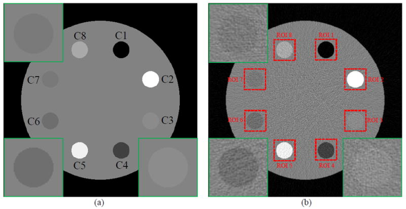
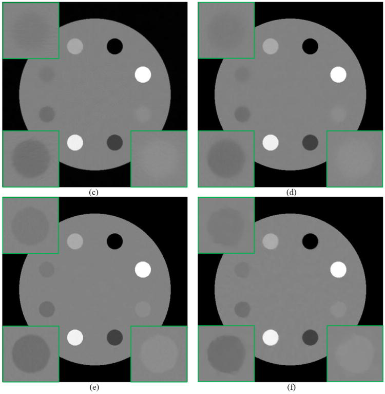
One slice of the clock phantom: (a) phantom; (b) FBP reconstruction from simulated noisy sinogram; (c) FBP+NLM filtering from simulated noisy sinogram (h=0.012); (d) PWLS-NLM reconstruction from simulated noisy sinogram (β=5×10⁶, h=0.008); (e) PWLS-adaptiveNLM reconstruction from simulated noisy sinogram (β=5×10⁶, s=5×10⁻⁴, t=4×10⁻⁶); (f) PWLS-TV reconstruction from simulated noisy sinogram (β=2×10³). All the images are displayed with the same window.
3.1.2. Noise reduction performance
To evaluate the noise reduction performance of the different reconstruction methods, two quantitative metrics were employed. According to Table 2, the proposed PWLS-adaptiveNLM method offers the highest PSNR and lowest NMSE, and therefore outperforms other methods in term of noise reduction, which is consistent with the visual inspection.
Table 2.
Noise reduction performance of the five reconstruction methods for the clock phantom
| Metrics | FBP | FBP+NLM filtering | PWLS-NLM | PWLS-adaptiveNLM | PWLS-TV |
|---|---|---|---|---|---|
| PSNR (dB) | 29.32 | 36.15 | 44.25 | 44.87 | 42.69 |
| NMSE (1e-4) | 129.12 | 26.80 | 4.15 | 3.61 | 5.95 |
3.1.3. Assessing local image quality
In order to evaluate the performance of different methods on the reconstruction of fine structures, we chose eight ROIs in the clock phantom, as labeled by the red rectangles in Figure 1(b). Since the FBP reconstructed image was obviously worse than those by the other four methods due to the excessive noise, we excluded it and only compared the local image quality by the other four methods. The quantitative results with RMSE and UQI are illustrated in Figure 2. Still, the proposed PWLS-adaptiveNLM has the best local image quality for the eight detailed ROIs with the lowest RMSE and highest UQI. The UQI quantifies the noise, spatial resolution, and texture correlation. From Figure 2(b), it is noted that the UQI values of the high-contrast ROIs (including C1: -100%, C2: +150%, C4: -50%, C5: +85%, C8: +30%) by the four different methods are relatively high and comparable, while the UQI values of the low-contrast ROIs (including C3: +7%, C6: -15%, C7: -7%) by the four different methods are relatively low and differ substantially. These results suggest that the low-contrast objects are more difficult to recover but the PWLS-adaptiveNLM method performed well in recovering them. The merit is significant, since we know that the low-contrast objects reconstruction can be very critical in clinic.
Figure 2.
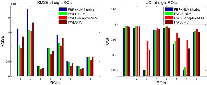
Performance comparison of the four methods on reconstruction of the eight ROIs labeled in Figure 1(b) with RMSE and UQI metrics. The corresponding methods are illustrated in figure legend.
3.2. Physical anthropomorphic torso phantom outcome
3.2.1. Visualization-based evaluation
Figure 3(a) shows one transverse image of the anthropomorphic torso phantom reconstructed by the FBP method from the averaged sinogram of 150 repeated scans, which serves as the ground truth image for evaluation. Figure 3(b)-(f) illustrates the reconstructed images by the FBP, FBP+NLM filtering, PWLS-NLM, PWLS-adaptiveNLM and PWLS-TV from a low-dose 40mAs sinogram. The FBP+NLM filtering method can suppress the noise pretty well, but there are still tiny streak artifacts in the image. The three PWLS methods outperform the FBP+NLM in terms of streak artifacts suppression, which can be attributed to the statistical modeling of the sinogram data. From the zoom-in views of the detailed regions, we can observe that the PWLS-adaptiveNLM method is superior to the PWLS-NLM and PWLS-TV on the reconstruction of the fine structures.
Figure 3.
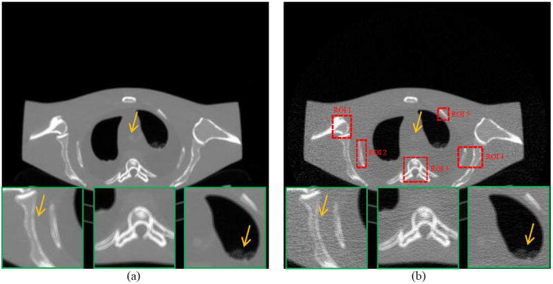
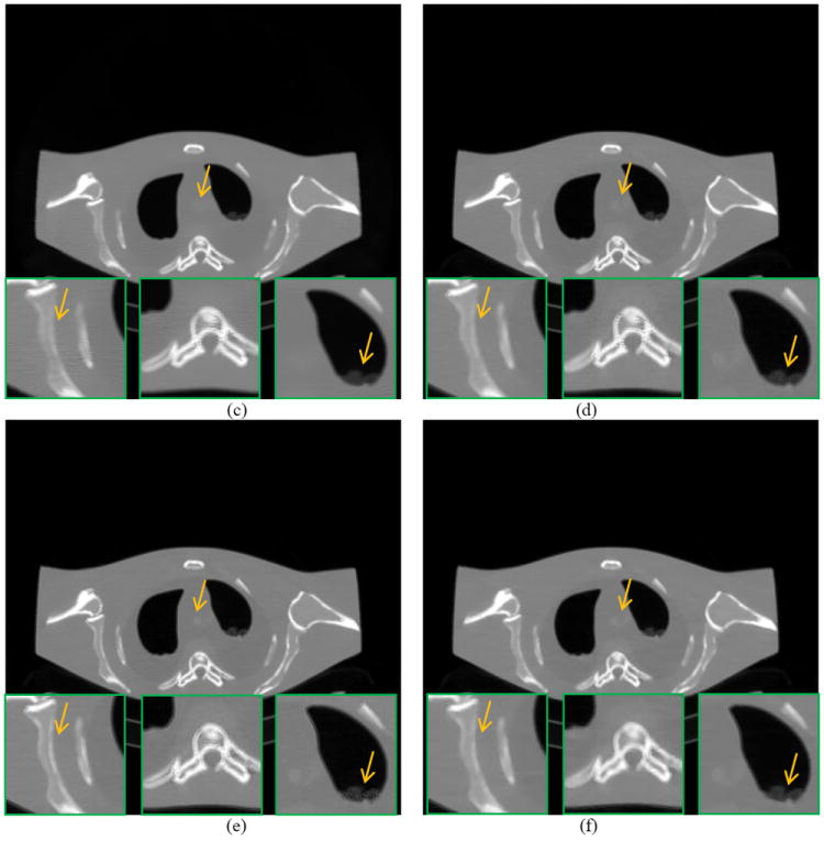
A reconstructed slice of the anthropomorphic torso phantom: (a) FBP reconstruction from the averaged sinogram; (b) FBP reconstruction from the 40mAs sinogram; (c) FBP+NLM filtering from the 40mAs sinogram (h=0.012); (d) PWLS-NLM reconstruction from the 40mAs sinogram (β=3×10⁵, h=0.008); (e) PWLS-adaptiveNLM reconstruction from the 40mAs sinogram (β=3×10⁵, s=5×10⁻⁴, t=4×10⁻⁶); (f) PWLS-TV reconstruction from the 40mAs sinogram (β=200). All the images are displayed with the same window.
3.2.2. Noise reduction performance
Table 3 lists the quantitative results of the five different reconstruction methods on the anthropomorphic torso phantom with PSNR and NMSE metrics. The proposed PWLS-adaptiveNLM method also demonstrates better performance than the other four methods on image noise reduction.
Table 3.
Noise reduction performance of the five reconstruction methods for the anthropomorphic torso phantom
| Metrics | FBP | FBP+NLM filtering | PWLS-NLM | PWLS-adaptiveNLM | PWLS-TV |
|---|---|---|---|---|---|
| PSNR (dB) | 31.00 | 38.91 | 39.17 | 39.39 | 39.09 |
| NMSE (1e-4) | 148.54 | 24.06 | 22.62 | 21.54 | 23.11 |
3.2.3. Assessing local image quality
To quantitatively demonstrate the benefits of the proposed PWLS-adaptiveNLM method, we compare the performance of the four methods on the reconstruction of ROIs with fine structures, which are labeled with red rectangles in Figure 3(b). The corresponding quantitative results based on the RMSE and UQI metrics are shown in Figure 4. Again, the PWLS-adaptiveNLM method yielded the lowest RMSE and the highest UQI for all the five detailed ROIs.
Figure 4.
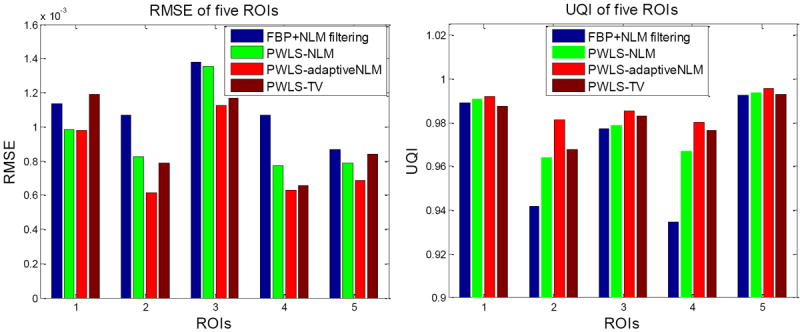
Performance comparison of the four methods on the reconstruction of detailed ROIs labeled in Figure 3(b) with RMSE and UQI metrics. The corresponding methods are illustrated in figure legend.
3.3. Clinical patient data outcome
The reconstructed images by the FBP, FBP+NLM filtering, PWLS-NLM, PWLS-adaptiveNLM and PWLS-TV from the ultra low-dose 20mAs sinogram of the patient are shown in Figure 5(a)-(e). We can see that the FBP+NLM filtering method cannot eliminate the streak artifacts in the image, while the three PWLS methods do not have such problem due to the statistical modeling of the sinogram data. However, the PWLS-TV exhibits slight patchy artifacts in the region indicated by the arrow, which is also reported in [17, 20]. From the zoom-in views of the three detailed regions, we can also see that the PWLS-adaptiveNLM method outperforms the other methods on the reconstruction of the fine structures.
Figure 5.
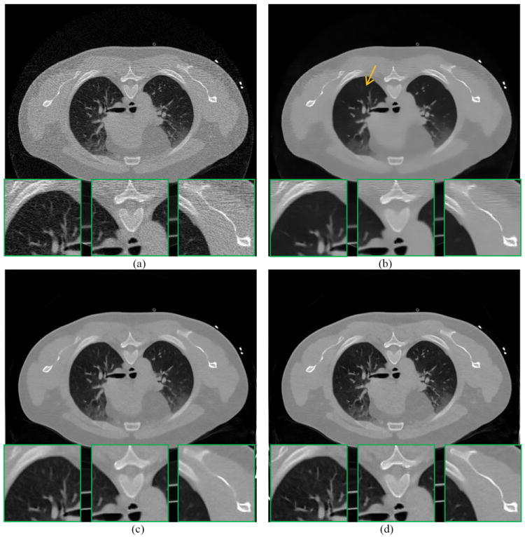
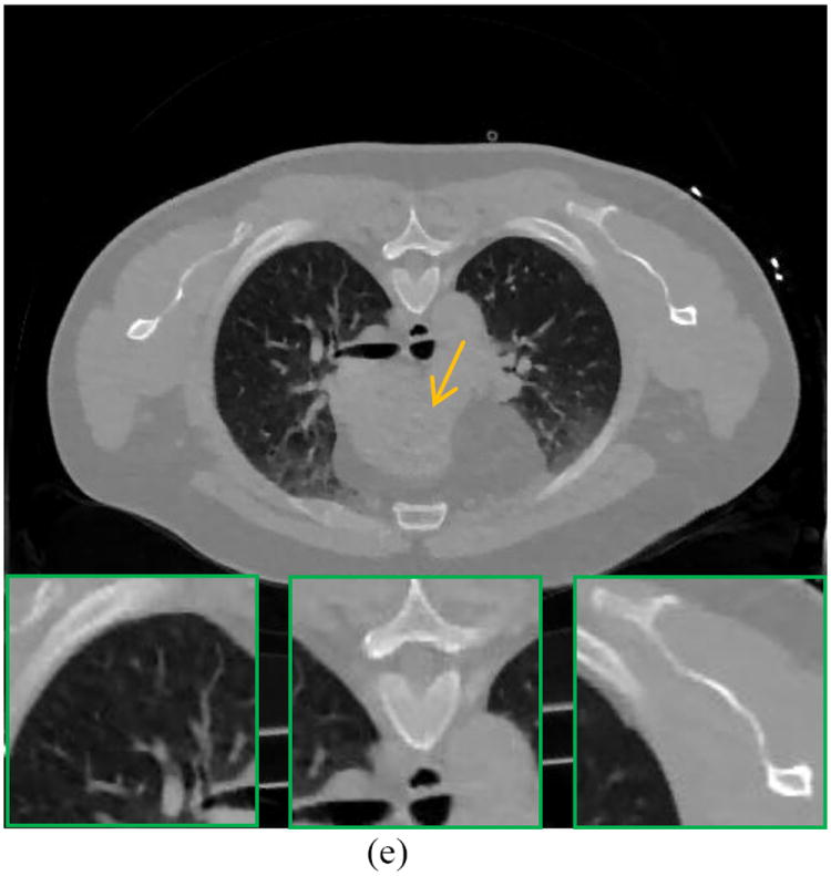
A reconstructed slice of the patient data: (a) FBP reconstruction from the 20mAs sinogram; (b) FBP+NLM filtering from the 20mAs sinogram (h=0.012); (c) PWLS-NLM reconstruction from the 20mAs sinogram (β=1×10⁵, h=0.008); (d) PWLS-adaptiveNLM reconstruction from the 20mAs sinogram (β=1×10⁵, s=1×10⁻³, t=4×10⁻⁶); (e) PWLS-TV reconstruction from the 20mAs sinogram (β=50). All the images are displayed with the same window.
However, for the patient study, we cannot implement the quantitative evaluations as the phantom studies due to the lack of ground truth image. Still, we observe that the patient study exhibits the same trend as the phantom studies through visual inspection.
4. Discussions and Conclusions
In this study, we proposed and validated an adaptive NLM-regularized statistical image reconstruction method for X-ray CT from low-dose acquisitions. One motivation of this work is that the traditional NLM filtering methods sometimes cannot completely remove the noise and streak artifacts in the low-dose CT images, especially when the streak artifacts are very severe. The NLM-regularized statistical image reconstruction method can mitigate this problem, partially due to the explicit statistical modeling of the projection data. However, the choice of the associated filtering parameter h as a spatially-invariant global constant in the NLM-based regularization may not be optimal for the reconstruction of the entire image. To further improve the reconstruction results, we proposed a novel strategy to determine locally optimal filtering parameter by considering local characteristics of the image, which made the NLM-based regularization to be adaptive. The experimental results with the PWLS-NLM and PWLS-adaptiveNLM methods proved that it is indeed necessary and beneficial to introduce the spatial adaptivity of the filtering parameter.
It is noted that the adaptive NLM-based regularization in this study is implemented in 2D domain. The implementation can be expanded to 3D space by setting the search-window and patch window to, for instance, 17×17×17 and 5×5×5 respectively for isotropic data. This may further improve the performance of the proposed method, although it would also increase the computation burden.
Also, it is noted that the proposed adaptive NLM regularization shares similar idea with the edge-preserving TV [40] and adaptive-weighted TV [41,42] regularization. Although using different mechanism to incorporate the spatial adaptivity, they essentially both consider local characteristics of the image to be reconstructed. However, the NLM-based regularization may have the advantage of better eliminating the patchy artifacts sometimes appearing in the TV-based regularization, due to the use of a larger neighborhood.
As any other proposed method, the presented PWLS-adaptiveNLM method also has some potential limitations. The first one is the parameters tuning. While the sizes of search-window and patch-window (also the standard deviation of the Gaussian kernel) do not show noticeable effects on the reconstructed image when they are set in a reasonable range and the parameter setting t = 4×10⁻⁶ in Eq. (7) works well, the strength parameter s in Eq. (7) seems need more manual tuning than the others. In this study, a typical range for s was found from 4×10⁻⁴ to 1×10⁻³. Further investigation on the strength parameter is needed. This is another topic in our future research plan.
Sharing the same challenges as other iterative reconstruction methods do, the proposed method also faces the limitation in computation efficiency due to the multiple re-projection and back-projection operation cycles between the projection data domain and image domain as well as the weighting coefficients calculation in each iterative circle. With constant improvement in fast computation via dedicated hardware and software, the computational efficiency could not be a major challenge in the future.
Acknowledgments
This work was partly supported by the NIH/NCI under grants #CA082402 and #CA143111. JM was partially supported by the NSF of China under grants # 81371544, #81000613 and #81101046. JW was supported in part by grants from the Cancer Prevention and Research Institute of Texas (RP110562-P2 and RP130109), a grant from the American Cancer Society (RSG-13-326-01-CCE) and a grant from NIH (R01EB020366). HL was supported in part by the NSF of China grants #81230035 and #81071220.
Footnotes
Conflict of interest statement
No conflict of interest was declared by the authors.
References
- 1.http://www.imvinfo.com/index.aspx?sec=ct&.
- 2.Brenner D, Hall E. Computed tomography-an increasing source of radiation exposure. The New England Journal of Medicine. 2007;357:2277–2284. doi: 10.1056/NEJMra072149. [DOI] [PubMed] [Google Scholar]
- 3.Hsieh J. Computed tomography: principles, design, artifacts, and recent advances. Bellingham, WA: SPIE; 2009. [Google Scholar]
- 4.McCollough CH, Primak AN, Braun N, Kofler J, Yu L, Christner J. Strategies for reducing radiation dose in CT. Radiologic Clinics of North America. 2009;47(1):27–40. doi: 10.1016/j.rcl.2008.10.006. [DOI] [PMC free article] [PubMed] [Google Scholar]
- 5.Yu L, Liu X, Leng S, Kofler JM, Ramirez-Giraldo JC, Qu M, et al. Radiation dose reduction in computed tomography: techniques and future perspective. Imaging in Medicine. 2009;1(1):65–84. doi: 10.2217/iim.09.5. [DOI] [PMC free article] [PubMed] [Google Scholar]
- 6.Liang Z, Lu H, Li X. 7,187,794. Noise Treatment of Low-dose Computed Tomography Projections and Images. Serial Number 10/273,927, B2 (filed in 2002 and approved in 2007)
- 7.Giraldo JC, Kelm ZS, Guimaraes LS, Yu L, Fletcher JG, Erickson BJ, McCollough CH. Comparative study of two image space noise reduction methods for Computed Tomography: bilateral filter and nonlocal means. Proceedings of 31st Annual International conference of the IEEE EMBS; 2009. pp. 3529–3532. [DOI] [PubMed] [Google Scholar]
- 8.Chen Y, Yang Z, Hu Y, Yang G, Zhu Y, Li Y, Chen W, Toumoulin C. Thoracic low-dose CT image processing using an artifact suppressed large-scale nonlocal means. Phys Med Biol. 2012;57(9):2667–2688. doi: 10.1088/0031-9155/57/9/2667. [DOI] [PubMed] [Google Scholar]
- 9.Li Z, Yu L, Trzasko JD, Lake DS, Blezek DJ, Fletcher JG, McCollough CH, Manduca A. Adaptive nonlocal means filtering based on local noise level for CT denoising. Med Phys. 2014;41(1):011908. doi: 10.1118/1.4851635. [DOI] [PubMed] [Google Scholar]
- 10.Ma J, Huang J, Feng Q, Zhang H, Lu H, Liang Z, Chen W. Low-dose computed tomography image restoration using previous normal-dose scan. Med Phys. 2011;38:5713–5731. doi: 10.1118/1.3638125. [DOI] [PMC free article] [PubMed] [Google Scholar]
- 11.Zhang H, Wang J, Ma J, Lu H, Liang Z. Statistical models and regularization strategies in statistical image reconstruction of low-dose X-ray computed tomography: a survey. arXiv preprint, arXiv:1412.1732. 2014 [Google Scholar]
- 12.http://www.gehealthcare.com/dose/how-we-can-help/computed-tomography.html.
- 13.http://www.healthcare.siemens.com/computed-tomography/technologies-innovations/admire.
- 14.http://www.healthcare.philips.com/main/products/ct/products/imr/#.
- 15.Wang J, Li T, Lu H, Liang Z. Penalized weighted least-squares approach to sinogram noise reduction and image reconstruction for low-dose X-ray CT. IEEE Trans Med Imag. 2006;25(10):1272–1283. doi: 10.1109/42.896783. [DOI] [PMC free article] [PubMed] [Google Scholar]
- 16.Thibault JB, Sauer K, Bouman C, Hsieh J. A three-dimensional statistical approach to improved image quality for multislice helical CT. Med Phys. 2007;34:4526–4544. doi: 10.1118/1.2789499. [DOI] [PubMed] [Google Scholar]
- 17.Wang J, Li T, Xing L. Iterative image reconstruction for CBCT using edge-preserving prior. Med Phys. 2009;36:252–260. doi: 10.1118/1.3036112. [DOI] [PMC free article] [PubMed] [Google Scholar]
- 18.Tang J, Nett B, Chen G. Performance comparison between total variation (TV)-based compressed sensing and statistical iterative reconstruction algorithms. Phys Med Biol. 2009;54:5781–5804. doi: 10.1088/0031-9155/54/19/008. [DOI] [PMC free article] [PubMed] [Google Scholar]
- 19.Jia X, Dong B, Lou Y, Jiang SB. GPU-based iterative cone-beam CT reconstruction using tight frame regularization. Phys Med Biol. 2011;56:3787–3807. doi: 10.1088/0031-9155/56/13/004. [DOI] [PubMed] [Google Scholar]
- 20.Ouyang L, Solberg T, Wang J. Effects of the penalty on the penalized weighted least-squares image reconstruction for low-dose CBCT. Phys Med Biol. 2011;56:5535–5552. doi: 10.1088/0031-9155/56/17/006. [DOI] [PubMed] [Google Scholar]
- 21.Xu Q, Yu H, Mou X, Zheng L, Hsieh J, Wang G. Low-dose X-ray CT reconstruction via dictionary learning. IEEE Trans Med Imag. 2012;31:1682–1697. doi: 10.1109/TMI.2012.2195669. [DOI] [PMC free article] [PubMed] [Google Scholar]
- 22.Theriault-Lauzier P, Chen G. Characterization of statistical prior image constrained compressed sensing II: Application to dose reduction. Med Phys. 2013;40(2):021902. doi: 10.1118/1.4773866. [DOI] [PMC free article] [PubMed] [Google Scholar]
- 23.Zhang H, Han H, Wang J, Ma J, Liu Y, Moore W, Liang Z. Deriving adaptive MRF coefficients from previous normal-dose CT scan for low-dose image reconstruction via penalized weighted least-squares minimization. Med Phys. 2014;41(4):041916. doi: 10.1118/1.4869160. [DOI] [PMC free article] [PubMed] [Google Scholar]
- 24.Ma J, Zhang H, Gao Y, Huang J, Liang Z, Feng Q, Chen W. Iterative image reconstruction for cerebral perfusion CT using a pre-contrast scan induced edge-preserving prior. Phys Med Biol. 2012;57:7519–7542. doi: 10.1088/0031-9155/57/22/7519. [DOI] [PMC free article] [PubMed] [Google Scholar]
- 25.Tian Z, Jia X, Dong B, Lou Y, Jiang S. Low-dose 4DCT reconstruction via temporal nonlocal means. Med Phys. 2011;38:1359–1365. doi: 10.1118/1.3547724. [DOI] [PubMed] [Google Scholar]
- 26.Jia X, Tian Z, Lou Y, Sonke J, Jiang S. Four-dimensional cone beam CT reconstruction and enhancement using a temporal nonlocal means method. Med Phys. 2012;39:5592–5602. doi: 10.1118/1.4745559. [DOI] [PMC free article] [PubMed] [Google Scholar]
- 27.Zhang H, Ma J, Liu Y, Han H, Li L, Wang J, Liang Z. Nonlocal means-based regularizations for statistical CT reconstruction. Proc SPIE Medical Imaging. 2014;9033 doi: 10.1117/12.2043949. [DOI] [Google Scholar]
- 28.Zhang H, Ma J, Wang J, Liu Y, Lu H, Liang Z. Statistical image reconstruction for low-dose CT using nonlocal means-based regularization. Comput Med Imaging Graph. 2014;38(6):423–435. doi: 10.1016/j.compmedimag.2014.05.002. [DOI] [PMC free article] [PubMed] [Google Scholar]
- 29.Buades A, Coll B, Morel J. A non-local algorithm for image denoising. IEEE Computer Vision and Pattern Recognition. 2005;2:60–65. [Google Scholar]
- 30.Buades A, Coll B, Morel J. A review of image denoising algorithms with a new one. Multiscale Model Simul. 2005;4(2):490–530. [Google Scholar]
- 31.Coupé P, Yger P, Prima S, Hellier P, Kervrann C, Barillot C. An optimized blockwise nonlocal means denoising filter for 3-D magnetic resonance images. IEEE Trans Med Imag. 2008;27:425–441. doi: 10.1109/TMI.2007.906087. [DOI] [PMC free article] [PubMed] [Google Scholar]
- 32.Ma J, Liang Z, Fan Y, Liu Y, Huang J, Chen W, Lu H. Variance analysis of x-ray CT sinograms in the presence of electronic noise background. Med Phys. 2012;39:4051–4065. doi: 10.1118/1.4722751. [DOI] [PMC free article] [PubMed] [Google Scholar]
- 33.Thibault JB, Bouman C, Sauer K, Hsieh J. A recursive filter for noise reduction in statistical iterative tomographic imaging. Proc of the SPIE/IS&T Symposium on Electronic Imaging Science and Technology-Computational Imaging; 2006. pp. 15–19. [Google Scholar]
- 34.Lou Y, Zhang X, Osher S, Bertozzi A. Image recovery via nonlocal operators. SIAM J Sci Comput. 2010;42(2):185–197. [Google Scholar]
- 35.Chen Y, Ma J, Feng Q, Luo L, Shi P, Chen W. Nonlocal prior Bayesian tomographic reconstruction. J Math Imag Vis. 2008;30(2):133–146. [Google Scholar]
- 36.Coupé P, Manjón JV, Fonov V, Pruessner J, Robles M, Collins DL. Patch-based segmentation using expert priors: Application to hippocampus and ventricle segmentation. NeuroImage. 2011;54(2):940–954. doi: 10.1016/j.neuroimage.2010.09.018. [DOI] [PubMed] [Google Scholar]
- 37.Evans JD, Politte DG, Whiting BR, O’Sullivan JA, Williamson JF. Noise-resolution tradeoffs in x-ray CT imaging: A comparison of penalized alternating. Med Phys. 2011;38:1444–58. doi: 10.1118/1.3549757. [DOI] [PMC free article] [PubMed] [Google Scholar]
- 38.La Rivière PJ, Billmire DM. Reduction of noise-induced streak artifacts in X-ray computed tomography through spline-based penalized-likelihood sinogram smoothing. IEEE Trans Med Imag. 2005;24:105–11. doi: 10.1109/tmi.2004.838324. [DOI] [PubMed] [Google Scholar]
- 39.Wang Z, Bovik A. A universal image quality index. IEEE Signal Process Letter. 2002;9:81–84. [Google Scholar]
- 40.Tian Z, Jia X, Yuan K, Pan T, Jiang SB. Low-dose CT reconstruction via edge-preserving total variation regularization. Phys Med Biol. 2011;56:5949–5967. doi: 10.1088/0031-9155/56/18/011. [DOI] [PMC free article] [PubMed] [Google Scholar]
- 41.Liu Y, Ma J, Fan Y, Liang Z. Adaptive-weighted total variation minimization for sparse data toward low-dose x-ray computed tomography image reconstruction. Phys Med Biol. 2012;57(23):7923–7956. doi: 10.1088/0031-9155/57/23/7923. [DOI] [PMC free article] [PubMed] [Google Scholar]
- 42.Liu Y, Ma J, Zhang H, Wang J, Liang Z. Low-mAs X-ray CT image reconstruction by adaptive-weighted TV-constrained penalized re-weighted least-squares. Journal of X-ray Science and Technology. 2014;22(4):437–457. doi: 10.3233/XST-140437. [DOI] [PMC free article] [PubMed] [Google Scholar]


