Validity of Automated Choroidal Segmentation in SS-OCT and SD-OCT

Abstract

Purpose.

To evaluate the validity of a novel fully automated three-dimensional (3D) method capable of segmenting the choroid from two different optical coherence tomography scanners: swept-source OCT (SS-OCT) and spectral-domain OCT (SD-OCT).

Methods.

One hundred eight subjects were imaged using SS-OCT and SD-OCT. A 3D method was used to segment the choroid and quantify the choroidal thickness along each A-scan. The segmented choroidal posterior boundary was evaluated by comparing to manual segmentation. Differences were assessed to test the agreement between segmentation results of the same subject. Choroidal thickness was defined as the Euclidian distance between Bruch's membrane and the choroidal posterior boundary, and reproducibility was analyzed using automatically and manually determined choroidal thicknesses.

Results.

For SS-OCT, the average choroidal thickness of the entire 6- by 6-mm² macular region was 219.5 μm (95% confidence interval [CI], 204.9–234.2 μm), and for SD-OCT it was 209.5 μm (95% CI, 197.9–221.0 μm). The agreement between automated and manual segmentations was high: Average relative difference was less than 5 μm, and average absolute difference was less than 15 μm. Reproducibility of choroidal thickness between repeated SS-OCT scans was high (coefficient of variation [CV] of 3.3%, intraclass correlation coefficient [ICC] of 0.98), and differences between SS-OCT and SD-OCT results were small (CV of 11.0%, ICC of 0.73).

Conclusions.

We have developed a fully automated 3D method for segmenting the choroid and quantifying choroidal thickness along each A-scan. The method yielded high validity. Our method can be used reliably to study local choroidal changes and may improve the diagnosis and management of patients with ocular diseases in which the choroid is affected.

The assessment of regional choroidal changes is of great interest. We show high validity for a fully automated and three-dimensional, highly reproducible method for segmentation and quantification of choroidal thickness of each A-scan in swept-source and spectral-domain OCT images.

The choroid provides oxygen and nourishment to the outer retinal layers and is crucial for metabolic activity in the retina.¹ Choroidal changes are associated with many eye diseases, such as age-related macular degeneration (AMD),² age-related choroidal atrophy,³ central serous retinopathy,⁴ and choroiditis. It has been also reported that choroidal thickness increases during childhood and decreases during adulthood.^5,6 Accurately and automatically measuring choroidal thickness is therefore of great interest. Spectral-domain optical coherence tomography (SD-OCT) provides a cross-sectional, three-dimensional (3D), microscale depiction of ocular tissues⁷ and clearly distinguishable retinal layers, as shown in Figure 1. However, without the use of enhanced depth imaging or image enhancement techniques, visualization of the choroid, including choroid–sclera junction, remains challenging (see Fig. 1). Due to the high backscatter by the retinal pigment epithelium layer (RPE), the intensity contrast in the choroid region can be insufficient for applying straightforward image analysis algorithms.

Figure 1.

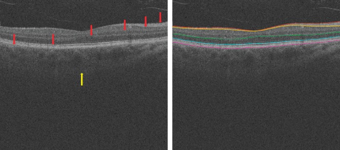
In the standard clinically available SD-OCT scans, retinal layer structures are clear (red arrows), but the posterior choroidal boundary is difficult to distinguish (yellow arrow). At right, the surfaces from top to bottom are internal limiting membrane, the transition between retinal nerve fiber layer and ganglion cell layer, outer boundary of outer plexiform layer, boundary of myoid and ellipsoid of inner segments, and Bruch's membrane.

Swept-source OCT (SS-OCT) allows increased scanning speed.⁸ In many SS-OCT prototype systems, a longer central wavelength (1060 vs. 840 nm in SD-OCT) is adopted to allow deeper penetration through the RPE. Consequently, the choroid–sclera boundary has higher contrast in SS-OCT (see Fig. 2). We and others have previously developed fully automated 3D algorithms for segmenting choroid on standard clinically available SD-OCT scans.^9–14 In our approach, choroidal thickness was estimated by defining the Euclidian distance between the enveloping surfaces of a choroidal vasculature segmentation (see Fig. 3).

Figure 2.

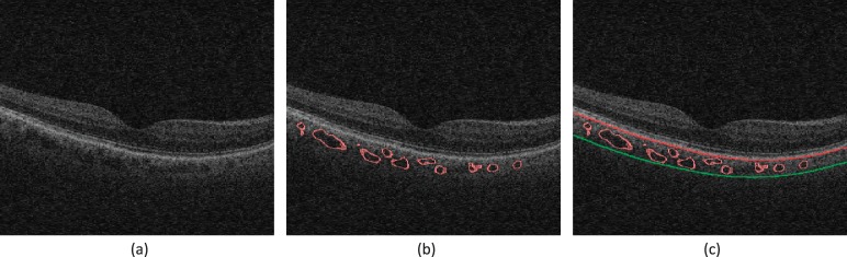
Segmentation results from the previous method on clinically available SD-OCT image (Zeiss Cirrus; EDI mode was not used): (a) Original B-scan; (b) 3D choroidal vasculature segmentation; (c) the outer boundary of choroidal vasculature is estimated using thinplate-spline surface fitting, real segmentation of choroidal–scleral interface was not achieved.

Figure 3.

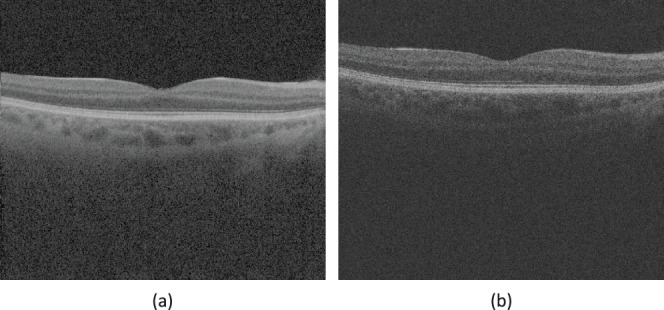
Swept-source OCT and spectral-domain OCT show difference of intensity contrast around choroidal–scleral interface. An example of the difference of intensity contrast at the same location from the same eye in (a) SS-OCT image data and in (b) SD-OCT image data.

The purpose of this study was to develop and evaluate the validity of a fully automated 3D method capable of segmenting the choroid over the entire scan and quantifying choroidal thicknesses of the macula in both SS-OCT and SD-OCT image data of the same subjects, without a preceding vasculature segmentation step, so that choroidal thickness can be measured for each A-scan.

Methods

Subject and Data Collection

The Rotterdam Study is a prospective population-based cohort study that investigates chronic diseases in the middle-aged and elderly.¹⁵ Inhabitants of Ommoord, a suburb of Rotterdam, The Netherlands, were invited to participate in this study at three different times: 1989, 2000, and 2006. This resulted in three cohorts: Rotterdam Study I (n = 7983, aged 55 years and older), Rotterdam Study II (n = 3011, aged 55 years and older), and Rotterdam Study III (n = 3982, aged 45 years and older). Follow-up examinations took place every 2 to 4 years and are still ongoing.

For this study we included 108 randomly selected subjects from Rotterdam Study II (second follow-up round) and Rotterdam Study III (first follow-up round), who participated between April 3 and April 26, 2013. All participants underwent an extensive ophthalmologic examination including SS-OCT (Topcon Corp., Tokyo, Japan) and SD-OCT (Topcon Corp.) imaging. Subjects were imaged on one day, once using SD-OCT and twice using SS-OCT. Enhanced Depth Imaging (EDI) mode was not used.¹⁶ In between scans, the head was lifted from the chin rest and subjects were asked to relax for no more than 15 minutes. Each volume scan was 512 (width of B-scan) × 128 (number of B-scans) × 885 (height of B-scan) voxels, corresponding to physical dimensions of approximately 6.0 × 6.0 × 2.3 mm³; the voxel size was 11.72 × 46.88 × 2.60 μm³. The mean age of the 108 subjects was 61.4 (±SD of 5.2; range, 52–78 years), with 45 male and 63 female subjects (41.7% and 58.3%, respectively). Over 92% of the participants were of European descent. Best corrected visual acuity (BCVA) was measured using the Lighthouse Distance Visual Acuity test, a corrected Early Treatment Diabetic Retinopathy Study chart.¹⁷ Best corrected visual acuity was impaired (BCVA ≤ 0.50, decimal notation was 20) in three eyes of 3 subjects due to cataract in two eyes and amblyopia in one eye. Mean spherical equivalent (SphE) was calculated using a standard formula (SphE = spherical value + 0.5 × cylinder). Mean SphE of the 108 subjects was 0.02 diopters (D) (±SD of 3.8 D; range, −10.7 to 9.6 D). Mean axial eye length (Lenstar; Haag-Streit Diagnostics, Koeniz, Switzerland) was 23.6 mm (±SD of 1.2; range, 20.80–26.39 mm). According to the fundus photographs and OCT scans, none of the included eyes showed retinal pathology in the posterior pole. Volumetric scan data were de-identified before image analysis. The Rotterdam Study has been approved by the Medical Ethics Committee of the Erasmus Medical Center and by the Ministry of Health, Welfare and Sport of The Netherlands, implementing the “Wet Bevolkingsonderzoek: ERGO (Population Studies Act: Rotterdam Study).” All participants provided written informed consent to participate in the study and to obtain information from their treating physicians. De-identified volume scans were transferred to the University of Iowa XNAT image database for offline processing.¹⁸ The study adhered to the tenets of the Declaration of Helsinki.

Choroidal Segmentation

We have developed a three-stage segmentation approach. First, to reduce the geometric distortion of the choroid layer caused by the position of the OCT scanner's optical axis relative to the subject's optical axis, an angle adjustment approach was applied to the original OCT volume,¹⁹ as shown in Figure 4b. Bruch's membrane (BM) was transformed to a relatively flat surface in the OCT image volume.²⁰ Second, BM was modeled as a convex arc on each B-scan, and the radius of this convex arc was computed using the average physical size of a human eyeball.²¹ A shape-prior–based soft-constraint graph-search method was employed to segment BM by utilizing this arc model²² (see Fig. 4c). In the third stage, the choroid layer was identified immediately beneath BM. A sufficiently large subvolume containing the choroid layer was selected as the target region to apply choroidal segmentation. A combined graph-cut-graph-search method was utilized to segment choroidal surfaces (see Fig. 4d). Intensity contrast was expected to be present around the choroidal posterior boundary, and vertical intensity gradient image was thus used to form the cost functions. To ensure the continuity of the segmented surface, smoothness constraints were adopted between neighboring A-scans. Due to the unequal voxel dimensions in the OCT volume scan (512 voxels in temporal–nasal direction and 128 voxels in superior–inferior direction), anisotropic smoothness constraints were established. More relaxed constraints were applied along the low-resolved direction (superior-inferior), and less relaxed constraints were employed along the high-resolved direction (temporal-nasal). The choroidal posterior boundary was subsequently segmented by graph optimization via identifying the minimum s-t cut in the employed geometric graph (see Appendix).

Figure 4.

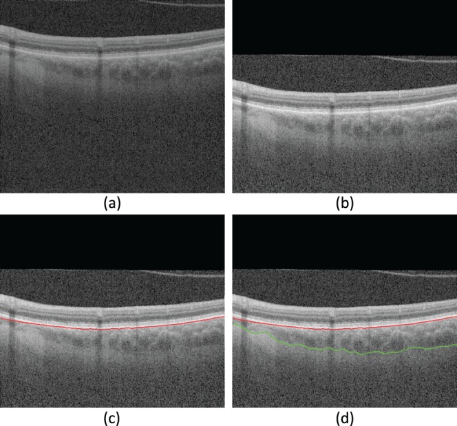
Three-dimensional choroidal segmentation using our proposed method. (a) An example B-scan from the original data; (b) the B-scan after applying the angle adjustment; (c) Bruch's membrane segmentation result; (d) choroidal posterior segmentation result. The red curve is the segmentation of Bruch's membrane; the green curve is the segmentation of choroidal posterior boundary. Though only a single B-scan is shown, the method operates in 3D across all B-scans.

Validation of the Choroidal Segmentation

The central B-scan and a random B-scan were extracted from each volumetric image. An experienced OCT analyst (GHSB) masked to the algorithm output manually segmented the choroidal posterior boundary on all selected B-scans. For each A-scan, the position of the segmented surface was defined as the depth from the top of the volumetric image in voxel domain. The outcome measure was the absolute and relative differences between the positions of the automated and manual segmentation results of the choroidal posterior boundary on two manually marked B-scans for each volumetric image. The relative difference was defined as automated value minus manual value. Bland-Altman plots were used to assess effect size on discrepancy: The relative differences were plotted against the mean position of automatically and manually segmented surfaces. A 95% limit of agreement (LOA) was defined as the average difference ± 1.96 × standard deviation of the difference, that is, the degree of agreement between automatically and manually segmented choroidal posterior boundaries. As described previously,²³ systematic error (SE) limit and total error (TE) limit were defined. The 95% confidence interval (95% CI) of the relative difference was compared with the predefined SE limit, and the 95% CI of LOA was compared with the predefined TE limit. In order to further test the systematic bias in the automated algorithm, a paired t-test was performed on the difference between the manual and automated segmentation results. To eliminate the possible systematic bias in the proposed method, a 3-fold cross-validation approach²⁴ was applied on the results of the proposed method (see Appendix).

Thickness Assessment

The choroidal thickness was calculated for each A-scan, defined as the Euclidian distance between BM and the posterior surface of the choroid. Choroidal thickness maps for the 6- × 6-mm² macula-centered region imaged by SS-OCT and SD-OCT scans were then created. The average thicknesses were reported in micrometers, with 95% CI. In addition to the average choroidal thickness for the 6- × 6-mm² macula-centered region, the fovea location was automatically detected using the Iowa Reference Algorithm²⁰ and the subfoveal choroidal thickness was determined.

Reproducibility Assessment of the Choroidal Thickness

For each subject, choroidal thickness was computed from two SS-OCT scans and one SD-OCT scan over the entire 6- × 6-mm² macula-centered region. Reproducibility analysis of the choroidal thickness was performed on the repeated SS-OCT scans and between SS-OCT and SD-OCT scans. To evaluate the test–retest reproducibility in repeated SS-OCT images, coefficients of variation (CV) and intraclass correlation coefficients (ICC) of the average choroidal thicknesses from automated and manual segmentation methods were determined using the root mean square (RMS) approach.²⁵ Similarly, the RMS CV and ICC between the average choroidal thicknesses from two SS-OCT scans and that of SD-OCT thickness were computed as well. To further test the algorithm on those scans with thicker choroids, subjects with subfoveal choroidal thickness greater than 300 μm were selected for the validity analyses, including thickness assessment and reproducibility assessment.

Comparison Between Proposed Method and Previous Method

We have previously reported an automated method for segmenting choroidal vasculature and estimating the posterior boundary of the choroidal vasculature using a Hessian vesselness analysis and thin-plate-spline surface fitting approach in a sequential fashion. In order to compare our new and previous results, we ran our earlier choroidal vasculature-based method on this dataset. The absolute and relative differences were computed between the automated segmentation results of the old method and the manual segmentation results. A paired t-test was then used to compare the absolute and relative differences between the new and old methods. A P value of 0.05 was considered significant.

Results

The agreement between automated and manual segmentations was high. The mean ± standard deviation of the relative differences for the entire dataset (216 SS-OCT images and 108 SD-OCT images) was −4.2 ± 20.5 μm (−1.6 ± 7.9 voxels); for the first SS-OCT dataset, the relative difference was −3.9 ± 18.7 μm (−1.5 ± 7.2 voxels); for the second SS-OCT dataset, the relative difference was −2.6 ± 19.5 μm (−1.0 ± 7.5 voxels); for the SD-OCT dataset, the relative difference was 6.2 ± 22.6 μm (−2.4 ± 8.7 voxels).

As shown in the Bland-Altman plots (Fig. 5), the difference between automated and manual results (automated result minus manual result) is relatively small; approximately 95% of the difference values are located within the LOA. The 95% LOA for the entire dataset (216 SS-OCT images and 108 SD-OCT images) was [−17.0 μm, 13.8 μm]; for the first SS-OCT dataset, the 95% LOA was [−15.7 μm, 12.6 μm]; for the second SS-OCT dataset, the 95% LOA was [−15.7 μm, 13.8 μm]; for the SD-OCT dataset, the 95% LOA was [−19.5 μm, 14.8 μm].

Figure 5.

Difference assessment between automated and manual segmentations (Bland-Altman plots): (a) on entire datasets: 216 SS-OCT scans and 108 SD-OCT scans; (b) on the first SS-OCT set; (c) on the second SS-OCT set; (d) on the SD-OCT set. Black dashed lines represent the mean of relative difference between automated and manual segmentations and red dashed lines represent the 95% limits of agreement (LOA). Ninety-five percent confidence interval of the mean difference and 95% LOA are added on the left end of the corresponding dashed lines; blue dashed lines represent the predefined total error (TE) as 10% of the average thickness; green dashed lines represent the redefined systematic error (SE) as 3% of the average thickness.²²

The mean ± standard deviation of absolute differences for the entire dataset (216 SS-OCT images and 108 SD-OCT images) was 13.8 ± 15.6 μm (5.3 ± 6.0 voxels); for the first SS-OCT dataset, the absolute difference was 12.6 ± 14.4 μm (4.9 ± 5.5 voxels); for the second SS-OCT dataset, the absolute difference was 12.3 ± 15.4 μm (4.7 ± 5.9 voxels); for the SD-OCT dataset, the absolute difference was 16.6 ± 16.6 μm (6.4 ± 6.4 voxels).

The mean difference between automated and manual segmentations was significantly smaller than a predefined SE of 3% of average thickness, and the 95% LOAs were significantly smaller than a predefined TE of 10% of average thickness.²³ For the SD-OCT dataset, the mean difference between automated and manual segmentation was significantly less than the SE, but 95% LOA approached the TE with no significant difference (see Fig. 5).

According to the results of paired t-test between the manual and automated segmentations, a systematic bias was found in our proposed method (mean difference was −4.2 μm, P < 0.01). As shown in Figure 5, the systematic bias was small and did not exceed the predefined SE limit. A 3-fold cross-validation approach²⁴ was then applied on the results of the proposed method. Paired t-test was performed again on the adjusted automated results and manual segmentation results and the bias was eliminated (P = 0.72).

For the 6- × 6-mm² macula-centered region imaged by SS-OCT, average choroidal thickness was 219.5 μm (95% CI, 204.9–234.2 μm); and for SD-OCT it was 209.5 μm (95% CI, 197.9–221.0 μm), corresponding to subfoveal choroidal thicknesses on SS-OCT of 246.7 ± 97.9 μm (max was 457.6 μm; min was 83.2 μm) and on SD-OCT of 229.7 ± 82.1 μm; (max was 429.0 μm; min was 85.8 μm).

The RMS CV of the automatically determined average choroidal thickness of repeated SS-OCT scans was 3.3% (95% CI, 2.2%–4.1%) with an ICC of 0.98 (P < 0.001); see Figure 6a. The reproducibility between the manual segmentation of repeated SS-OCT scans showed an RMS CV of 3.8% (95% CI, 3.2%–4.4%) and ICC of 0.96 (P < 0.001) (see Fig. 6b). The automated method was not significantly better than the manual expert (P = 0.28). The RMS CV between automatically determined average choroidal thickness of two SS-OCT scans and one SD-OCT scan was 11.0% (95% CI, 8.0%–13.3%) with an ICC of 0.73 (P < 0.001) (see Fig. 7a). The RMS CV between the manually determined average choroidal thickness of two SS-OCT scans and that of one SD-OCT scan was 9.1% (95% CI, 7.7%–10.3%) with an ICC of 0.75 (P < 0.001) (see Fig. 7b); however, these differences between automated and manual segmentation CVs were not significant (P = 0.24).

Figure 6.

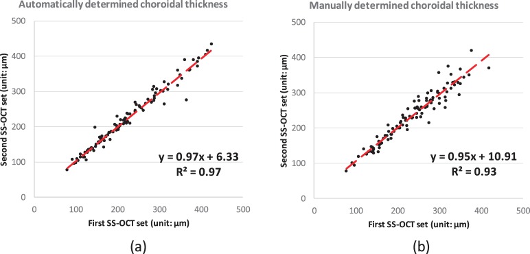
Correlation analysis of the choroidal thickness on entire 6-by-6 macular region between SS-OCT repeated scans: (a) automated segmentation; (b) manual segmentation.

Figure 7.

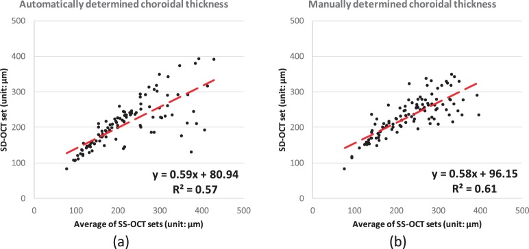
Correlation analysis of the choroidal thickness on entire 6-by-6 macular region between the mean of SS-OCT repeated scans and SD-OCT scan from the same subject: (a) automated segmentation; (b) manual segmentation.

Thirty-six subjects (72 SS-OCT scans and 36 SD-OCT scans) with subfoveal choroidal thickness greater than 300 μm were selected for the validity analyses. The average subfoveal choroidal thickness on SS-OCT in this subset was 363.8 μm (95% CI, 352.6–374.4 μm); it was 301.4 μm (95% CI, 274.1–328.7 μm) on SD-OCT. The average choroidal thickness over the entire 6- × 6-mm² macula-centered region imaged by SS-OCT in this subset was 305.8 μm (95% CI, 292.7–318.8 μm), and on SD-OCT it was 259.5 μm (95% CI, 239.0–279.7 μm). The RMS CV of the automatically determined average choroidal thickness of repeated SS-OCT scans with thick choroid was 3.4% (95% CI, 0.3%–4.7%) with an ICC of 0.93 (P < 0.001), The RMS CV between automatically determined average choroidal thickness of two SS-OCT scans and one SD-OCT scan with thick choroid was 16.4% (95% CI, 10.5%–20.7%) with an ICC of 0.18 (P = 0.1). The difference in CV between thinner and thicker choroids was not significant (P > 0.05).

For the old choroidal vasculature–based method, the mean ± standard deviation of the relative difference was −23.5 ± 34.4 μm (−9.0 ± 13.2 voxels) and the mean ± standard deviation of absolute difference was 33.4 ± 24.9 μm (12.8 ± 9.6 voxels)—for the entire dataset (216 SS-OCT images and 108 SD-OCT images). The proposed graph-based method in the current study outperformed the previous vasculature-based method (P < 0.001).

Discussion

The results of this study show the validity of a fully automated 3D method capable of segmenting the entire choroid and quantifying choroidal thickness of the macula in both SS-OCT and SD-OCT images of the same subjects, without a preceding vasculature segmentation step. Choroidal thickness can now be measured for each A-scan.

In the SS-OCT volumes, the volumetric data have sufficient image quality and high intensity contrast in the choroid region that our method successfully identifies the choroid borders in all SS-OCT scans accurately. In SD-OCT volumes, the intensity contrast is relatively lower, due to the increased backscattering of the retinal nerve fiber layer and RPE layer, caused by the shorter 840-nm wavelength used in these scanners. Swept-source OCT scanners use light with central wavelength of 1060 nm, providing enough intensity contrast and choroidal border information. As shown in Figure 8, the choroidal posterior boundaries are less well visualized in these types of SD-OCT scans. Despite the relative insufficiency of the choroidal border information in SD-OCT images, the agreement between automated and manual segmentations was still good.

Figure 8.

Two examples of subjects in whom the proposed choroidal segmentation of SD-OCT scans (left column) resulted in a large underestimation due to the lower contrast in that region, while segmentation of the SS-OCT scans of the same subjects (right column) led to adequate estimates.

The results of layer thickness assessment show that the average choroidal thickness obtained from SS-OCT scans is 219.5 μm (95% CI, 204.9–234.2 μm) and average choroidal thickness obtained from SD-OCT scans is 209.5 μm (95% CI, 197.9–221.0 μm), corresponding to subfoveal choroidal thicknesses on SS-OCT of 246.7 μm (max is 457.6 μm; min is 83.2 μm) and on SD-OCT of 229.7 μm (max is 429.0 μm; min is 85.8 μm). These thicknesses are comparable to the choroidal thickness reported by other studies.^26–28 In reproducibility analysis of the choroidal thickness, the proposed method shows outstanding reproducibility in SS-OCT: RMS CV is 3.3% (95% CI, 2.2%–4.1%) along with an ICC of 0.98. Meanwhile, the proposed method shows good reproducibility between SS-OCT and SD-OCT: RMS CV is 11.0% (95% CI, 8.0%–13.3%) along with an ICC of 0.73 (P < 0.001). However, for a subset of thicker choroids, the proposed method performed significantly better (P < 0.001) on SS-OCT than on SD-OCT.

The present graph-based method also outperforms (P < 0.001) the earlier vasculature-based method in reproducibility.⁹ In the earlier vessel-based method, approximately 50% of the SD-OCT scans were successfully segmented; the other half of the SD-OCT scans were automatically detected as lacking choroidal vessel information.⁹ Similar issues occur in the SD-OCT set of this new study. Inconsistency of the choroidal thickness is discovered in the correlation analysis between SS-OCT and SD-OCT. The correlation from automatically segmented choroid is shown by the R² of 0.57 with CV of 10.9%, and that from manually segmented choroid is shown by the R² of 0.61 with CV of 9.1% (no significant difference between choroidal thicknesses from manually and automatically segmentations, P = 0.24); see Figure 7. In the correlation analysis between automatically determined choroidal thicknesses of SS-OCT and SD-OCT images, some segmentations show a relatively large distance to the identity line, as shown in the region outlined with red solid segments in Figure 9. If we remove these problematic scans from analysis (20 out of 108 SD-OCT scans), the remaining scans show a reasonably good CV and ICC: For automatically segmented choroid, CV is 5.4% and ICC is 0.96 (P < 0.001); for manually segmented choroid, CV is 8.1% and ICC is 0.83 (P < 0.001). Thus, we may conclude that these 20 out of 108 SD-OCT scans do not have enough intensity contrast around the choroidal–scleral interface for automated or manual segmentations.

Figure 9.

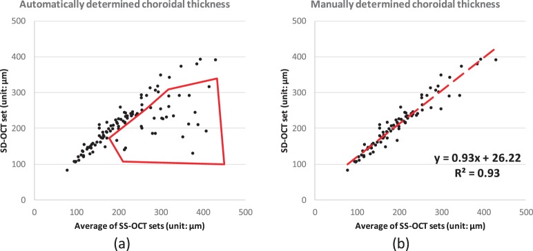
(a) The correlation between the choroidal thicknesses from SS-OCT and SD-OCT is fair as shown in Figure 7 (R² < 0.65). The region outlined by the red segments represents where some SD-OCT images do not have enough intensity contrast around choroidal–scleral interface; (b) the correlation is largely improved if we consider only those images with sufficient image quality.

In summary, the present method shows outstanding performance for segmenting choroid in all SS-OCT scans and good performance for segmenting choroid in more than 80% of SD-OCT scans (88 out of 108 scans). For the other 20 out of 108 SD-OCT scans, the automated method agrees highly with manual method, but the real accuracy of the segmentation results may be problematic. In this sense, SS-OCT imaging at 1060 nm is better for automated (and manual analysis) than SD-OCT imaging at 840 nm.

Recently, other groups have reported evaluations of semiautomated or automated segmentation of the choroid. These studies used surface fitting, surface smoothing, or postprocessing steps for identifying the choroidal borders. However, such approaches can produce only an approximate segmentation of choroid and deliver approximations of the overall average choroidal thickness. To the best of our knowledge, the method we report here is the first fully 3D automated method capable of accurately identifying the local thickness of the choroid for each A-scan. Figure 10 shows choroidal thickness maps and difference maps for one subject, demonstrating high reproducibility of choroidal thickness across OCT analyses of the same subject.

Figure 10.

Choroidal thickness maps and relative difference ratio maps from the same subject. (a) Thickness map of the first SS-OCT image; (b) thickness map of the second SS-OCT image; (c) absolute difference ratio map for the repeated SS-OCT images; (d) average thickness map of the repeated SS-OCT images; (e) thickness map of SD-OCT image; (f) absolute difference ratio map between the average SS-OCT image and SD-OCT image. The absolute difference ratio is computed as the result of the absolute difference along each A-scan divided by the average thickness between the thicknesses. The absolute difference ratio map between SS-OCT and SD-OCT images shows relatively larger difference than the absolute difference ratio map for repeated SS-OCT images.

There are several limitations to this study. First, due to the large dataset, only two B-scans—the central B-scan and a random B-scan—were selected from each volumetric image for manually identifying the choroidal posterior boundaries. As shown in the method details (see Appendix), the proposed graph-based method treats every B-scan evenly and the location of the random B-scans should represent all nonfoveal regions around macula across the entire dataset. Furthermore, the tests of RMS CV and ICC were performed on the entire 6- by 6-mm² macula-centered region. In a future study, we plan to evaluate all the B-scans if the manual segmentation is available for the entire macula-centered region. Second, the selected subjects were relatively old adults and did not have diseases such as central serous retinopathy (known to result in a thickened choroid). The presented method should also be evaluated in younger persons and persons with choroidal abnormalities. Such studies are currently being pursued. Third, all scans were scanned in horizontal (temporal-nasal) B-line mode. Each volumetric image had dimensions of 512 voxels temporal-nasally and 128 voxels superior-inferiorly. This required us to use anisotropic smoothness constraints as more relaxed constraints on superior-inferior direction and less relaxed constraints on temporal-nasal direction. Fourth, systematic differences were discovered between manual measurements and automated or semiautomated measurements when segmenting the choroidal posterior boundary.¹⁴

In summary, we have developed a fully automated 3D method for segmenting choroid layer and quantifying choroidal thickness in SS-OCT and SD-OCT volumetric data. The method yielded highly accurate segmentation results in SS-OCT and relatively good segmentation results in SD-OCT compared to a human expert. This is the first fully 3D automated method capable of accurately identifying the local thickness of the choroid in each A-scan. Potentially, our method may enhance the understanding of regional choroid changes and improve the diagnosis and management of patients with diseases in which the choroid is affected.

Appendix

Combined Graph-Cut-Graph-Search Method for Segmenting Posterior Boundary of Choroid

The choroid layer was identified immediately beneath Bruch's membrane. A sufficiently large subvolume containing the choroid layer was selected as the target region to apply choroidal segmentation. As described for the previous vasculature-based method,⁹ we applied multiscale Hessian matrix analysis on the selected subvolume. Three-dimensional vesselness map of the choroidal vasculature was then calculated. Probability values between 0 and 255 represented different vesselness of the choroidal vasculature. This vesselness contributed to the in-region cost in the graph-based method rather than a segmentation of the choroidal posterior boundary. Cost functions and graph representations were designed accordingly.

Cost Functions

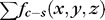
One on-surface cost was defined for the transitions from choroid to sclera. Due to the difference of the density between choroidal vasculature and sclera, the overall intensity of choroidal vasculature is lower than that of sclera. We introduced a dark-to-bright intensity gradient as for the surface between choroid and sclera. The on-surface cost formed one energy term in the cost function: . In-regions cost was defined as the region intensity difference inside and outside the vessel region of choroidal vasculature, forming the in-region energy term as .

The following equation shows the energy function of our graph-based method:

is the cost of relevant surface (transition), which is identical to the cost of a minimum closed set enveloped by the surface in the graph.

is defined as the region term of the energy function, which shows the likelihood of vertex-associated costs inside the vasculature regions.

Graph Representation

The main idea for solving the energy optimization problem was to reduce it to a maximum-flow minimum cut-graph problem. A graph G = (V, E) as the collection of vertices V and arcs E was constructed for representing the problem. The specific constructions were described as follows:

Surface-Specified Subgraphs.

Similar to the configuration reported previously,²⁹ node costs were assigned according to the intensity values from the original OCT image. For each surface, a directed subgraph as a part of the entire graph G was constructed to present a nonempty closed set. An optimal surface segmentation problem can be converted to solving a minimum closed set problem in this directed subgraph.

Object-Specified Subgraphs.

As discussed previously,^30,31 object and background nodes were predetermined by the detection of the choroidal vasculature. For the region term, t-links are assigned between terminals (source s, sink t) and vertices. The capacities of t-links were defined using the likelihood of whether the vertex was in object set. For the boundary term, n-links were assigned between neighboring vertices to represent whether these neighboring vertices should be in the same set (source set or sink set).

Multiobject Interactions.

As shown previously,³² certain maximum and minimum distances were considered as the prior knowledge of the relative position among multiple surfaces and objects. Intersubgraph arcs were introduced at the interacting areas to represent the maximum and minimum distances between adjacent structures.

3-Fold Cross Validation

In this study, systematic differences between the automated and manual segmentation results were tested using a paired t-test (P < 0.01). To eliminate the systematic bias in the proposed method, a 3-fold cross-validation approach was applied to the results of the proposed method. The original dataset (108 subjects) was randomly partitioned into three independent groups (folds): groups A, B, and C. Each group contained 36 subjects.

To adjust the segmentation results of group A, we first computed the average relative difference between automated and manual segmentation results in groups B and C. We used this average relative difference as the trained systematic bias, which was independent from group A. All automated segmentation results in group A were then adjusted by subtracting this independently trained systematic bias from groups B and C.

Similarly, to adjust segmentation results for group B, we used the trained systematic bias from groups A and C. To adjust segmentation results for group C, we used the trained systematic bias from groups A and B.

The adjusted automated segmentation results showed no significant differences when compared with manual segmentation results (P = 0.72).

References

- 1. Nickla DL,, Wallman J. The multifunctional choroid. Prog Retin Eye Res. 2010; 29: 144–168. [DOI] [PMC free article] [PubMed] [Google Scholar]
- 2. Zarbin MA. Current concepts in the pathogenesis of age-related macular degeneration. Arch Ophthalmol. 2004; 122: 598–614. [DOI] [PubMed] [Google Scholar]
- 3. Spaide RF. Age-related choroidal atrophy. Am J Ophthalmol. 2009; 147: 801–810. [DOI] [PubMed] [Google Scholar]
- 4. Wang M,, Munch IC,, Hasler PW,, Prünte C,, Larsen M. Central serous chorioretinopathy. Acta Ophthalmol. 2008; 86: 126–145. [DOI] [PubMed] [Google Scholar]
- 5. Ramrattan RS,, van der Schaft TL,, Mooy CM,, de Bruijn WC,, Mulder PG,, de Jong PT. Morphometric analysis of Bruch's membrane, the choriocapillaris, and the choroid in aging. Invest Ophthalmol Vis Sci. 1994; 35: 2857–2864. [PubMed] [Google Scholar]
- 6. Read SA,, Collins MJ,, Vincent SJ,, Alonso-Caneiro D. Choroidal thickness in childhood. Invest Ophthalmol Vis Sci. 2013; 54: 3586–3593. [DOI] [PubMed] [Google Scholar]
- 7. Nassif N,, Cense B,, Park B,, et al. In vivo high-resolution video-rate spectral-domain optical coherence tomography of the human retina and optic nerve. Opt Express. 2004; 12: 367–376. [DOI] [PubMed] [Google Scholar]
- 8. Yasuno Y,, Hong Y,, Makita S,, et al. In vivo high-contrast imaging of deep posterior eye by 1-um swept source optical coherence tomography and scattering optical coherence angiography. Opt Express. 2007; 15: 6121–6139. [DOI] [PubMed] [Google Scholar]
- 9. Zhang L,, Lee K,, Niemeijer M,, Mullins RF,, Sonka M,, Abràmoff MD. Automated segmentation of the choroid from clinical SD-OCT. Invest Ophthalmol Vis Sci. 2012; 53: 7510–7519. [DOI] [PMC free article] [PubMed] [Google Scholar]
- 10. Hu Z,, Wu X,, Ouyang Y,, Ouyang Y,, Sadda SR. Semiautomated segmentation of the choroid in spectral-domain optical coherence tomography volume scans. Invest Ophthalmol Vis Sci. 2013; 54: 1722–1729. [DOI] [PubMed] [Google Scholar]
- 11. Kajić V,, Esmaeelpour M,, Považay B,, Marshall D,, Rosin PL,, Drexler W. Automated choroidal segmentation of 1060 nm OCT in healthy and pathologic eyes using a statistical model. Biomed Opt Express. 2012; 3: 86–103. [DOI] [PMC free article] [PubMed] [Google Scholar]
- 12. Tian J,, Marziliano P,, Baskaran M,, Tun TA,, Aung T. Automatic segmentation of the choroid in enhanced depth imaging optical coherence tomography images. Biomed Opt Express. 2013; 4: 397–411. [DOI] [PMC free article] [PubMed] [Google Scholar]
- 13. Matsuo Y,, Sakamoto T,, Yamashita T,, Tomita M,, Shirasawa M,, Terasaki H. Comparisons of choroidal thickness of normal eyes obtained by two different spectral-domain OCT instruments and one swept-source OCT instrument. Invest Ophthalmol Vis Sci. 2013; 54: 7630–7636. [DOI] [PubMed] [Google Scholar]
- 14. Alonso-Caneiro D,, Read SA,, Collins MJ. Automatic segmentation of choroidal thickness in optical coherence tomography. Biomed Opt Express. 2013; 4: 2795–2812. [DOI] [PMC free article] [PubMed] [Google Scholar]
- 15. Hofman A,, DarwishMurad S,, van Duijn CM,, et al. The Rotterdam Study: 2014 objectives and design update. Eur J Epidemiol. 2013; 28: 889–926. [DOI] [PubMed] [Google Scholar]
- 16. Spaide RF,, Koizumi H,, Pozonni MC. Enhanced depth imaging spectral-domain optical coherence tomography. Am J Ophthalmol. 2008; 146: 496–500. [DOI] [PubMed] [Google Scholar]
- 17. ETDRS Research Group. Early Treatment Diabetic Retinopathy Study Manual of Operations. Springfield, VA: National Technical Information Service; 1985: 1–74. [Google Scholar]
- 18. Wahle A,, Lee K,, Harding AT,, et al. Extending the XNAT archive tool for image and analysis management in ophthalmology research. In: Proc. SPIE 8674, Medical Imaging 2013: Advanced PACS-based Imaging Informatics and Therapeutic Applications; February 9, 2013; Lake Buena Vista, FL. 86740M. doi:http://dx.doi.org/10.1117/12.2007966.
- 19. Lee K,, Sonka M,, Kwon YH,, Garvin MK,, Abràmoff MD. Adjustment of the retinal angle in SD-OCT of glaucomatous eyes provides better intervisit reproducibility of peripapillary RNFL thickness. Invest Ophthalmol Vis Sci. 2013; 54: 4808–4812. [DOI] [PMC free article] [PubMed] [Google Scholar]
- 20. Garvin MK,, Abràmoff MD,, Wu X,, Russell SR,, Burns TL,, Sonka M. Automated 3-D intraretinal layer segmentation of macular spectral-domain optical coherence tomography images. IEEE Trans Med Imaging. 2009; 28: 1436–1447. [DOI] [PMC free article] [PubMed] [Google Scholar]
- 21. Riordan-Eva P. Anatomy & embryology of the eye. : Riordan-Eva P,, Whitcher J, Vaughan & Asbury's General Ophthalmology. New York, NY: Lange Medical Books/McGraw-Hill Medical Pub. Division; 2008: chapter 1. [Google Scholar]
- 22. Chen X,, Niemeijer M,, Zhang L,, Lee K,, Abramoff MD,, Sonka M. Three-dimensional segmentation of fluid-associated abnormalities in retinal OCT: probability constrained graph-search-graph-cut. IEEE Trans Med Imaging. 2012; 31: 1521–1531. [DOI] [PMC free article] [PubMed] [Google Scholar]
- 23. Stöckl D,, Rodríguez Cabaleiro D,, Van Uytfanghe K,, Thienpont LM. Interpreting method comparison studies by use of the Bland–Altman plot: reflecting the importance of sample size by incorporating confidence limits and predefined error limits in the graphic. Clin Chem. 2004; 50: 2216–2218. [DOI] [PubMed] [Google Scholar]
- 24. Bishop CM. Pattern Recognition and Machine Learning. Vol 1 New York: Springer; 2006: 32–33. [Google Scholar]
- 25. Agawa T,, Miura M,, Ikuno Y,, et al. Choroidal thickness measurement in healthy Japanese subjects by three-dimensional high-penetration optical coherence tomography. Graefes Arch Clin Exp Ophthalmol. 2011; 249: 1485–1492. [DOI] [PubMed] [Google Scholar]
- 26. Esmaeelpour M,, Povazay B,, Hermann B,, et al. Three-dimensional 1060-nm OCT: choroidal thickness maps in normal subjects and improved posterior segment visualization in cataract patients. Invest Ophthalmol Vis Sci. 2010; 51: 5260–5266. [DOI] [PubMed] [Google Scholar]
- 27. Shin JW,, Shin YU,, Lee BR. Choroidal thickness and volume mapping by a six radial scan protocol on spectral-domain optical coherence tomography. Ophthalmology. 2012; 119: 1017–1023. [DOI] [PubMed] [Google Scholar]
- 28. McCourt EA,, Cadena BC,, Barnett CJ,, Ciardella AP,, Mandava N,, Kahook MY. Measurement of subfoveal choroidal thickness using spectral domain optical coherence tomography. Ophthalmic Surg Lasers Imaging. 2010; 41 (suppl): S28–S33. [DOI] [PubMed] [Google Scholar]
- 29. Li K,, Wu X,, Chen DZ,, Sonka M. Optimal surface segmentation in volumetric images—a graph-theoretic approach. IEEE Trans Pattern Anal Mach Intell. 2006; 28: 119–134. [DOI] [PMC free article] [PubMed] [Google Scholar]
- 30. Boykov Y,, Kolmogorov V. An experimental comparison of min-cut/max-flow algorithms for energy minimization in vision. IEEE Trans Pattern Anal Mach Intell. 2004; 26: 1124–1137. [DOI] [PubMed] [Google Scholar]
- 31. Boykov Y,, Funka-Lea G. Graph cuts and efficient ND image segmentation. Int J Comput Vis. 2006; 70: 109–131. [Google Scholar]
- 32. Yin Y,, Zhang X,, Williams R,, Wu X,, Anderson DD,, Sonka M. LOGISMOS—layered optimal graph image segmentation of multiple objects and surfaces: cartilage segmentation in the knee joint. IEEE Trans Med Imaging. 2010; 29: 2023–2037. [DOI] [PMC free article] [PubMed] [Google Scholar]