To sort or not to sort: the impact of spike-sorting on neural decoding performance

Abstract

Objective

Brain-computer interfaces (BCIs) are a promising technology for restoring motor ability to paralyzed patients: spiking-based BCIs have successfully been used in clinical trials to control multi-degree-of-freedom robotic devices. Current implementations of these devices require a lengthy spike-sorting step, which is an obstacle to moving this technology from the lab to the clinic. A viable alternative is to avoid spike-sorting, treating all threshold crossings of the voltage waveform on an electrode as coming from one putative neuron. It is not known, however, how much decoding information might be lost by ignoring spike identity.

Approach

We present a full analysis of the effects of spike-sorting schemes on decoding performance. Specifically, we compare how well two common decoders, the optimal linear estimator and the Kalman filter, reconstruct the arm movements of non-human primates performing reaching tasks, when receiving input from various sorting schemes. The schemes we tested included: using threshold crossings without spike-sorting; expertsorting discarding the noise; expert-sorting, including the noise as if it were another neuron; and automatic spike-sorting using waveform features. We also decoded from a joint statistical model for the waveforms and tuning curves, which does not involve an explicit spike-sorting step.

Main results

Discarding the threshold crossings that cannot be assigned to neurons degrades decoding: no spikes should be discarded. Decoding based on spike-sorted units outperforms decoding based on electrodes voltage crossings: spike-sorting is useful. The four waveform based spike-sorting methods tested here yield similar decoding efficiencies: a fast and simple method is competitive. Decoding using the joint waveform and tuning model shows promise but is not consistently superior.

Significance

Our results indicate that simple automated spikesorting performs as well as computationally or manually more intensive methods, which is crucial for clinical implementation of BCIs.

1. Introduction

A motor brain-computer interface (BCI) creates a link between recorded neural activity and the movement of a neuroprosthetic device (Schwartz 2007). One class of BCI infers motor intention from the activity of populations of neurons recorded with a microelectrode array. These spiking-based BCIs have shown impressive performance both in the lab (Serruya et al. 2002, Carmena et al. 2003, Mulliken et al. 2008, Velliste et al. 2008, Suminski et al. 2010, Gilja et al. 2012), and in early stage clinical trials with human patients (Hochberg et al. 2006, Hochberg et al. 2012, Collinger et al. 2013).

A major challenge for spiking-based BCIs is spike-sorting. Since each electrode on a microelectrode array can record the combined signals of multiple neurons together with noise, electrode arrays can track the spiking activity of hundreds of neurons at a time. The traditional approach is to first retrieve single-neuron activity by sorting spikes, and then decode movement kinematics using models describing their dependence on the activity of individual neurons. Spike-sorting is a difficult task and many methods exist (Lewicki 1998, Sahani 1999, Harris et al. 2000, Quiroga 2007, Gibson et al. 2012, Ge & Farina 2013). Achieving a high degree of accuracy requires computationally intensive algorithms, large amounts of data, and expert manual processing. The manual processing step is problematic for transitioning BCI devices from the lab to the clinic, as are computationally demanding algorithms, since decoding must proceed in real-time. Nowadays, a popular choice in the lab is to avoid spike-sorting altogether, and treat each electrode as a single putative neuron. This requires no data storing or processing, which is fast and easy, and therefore desirable for clinical use (Fraser et al. 2009, Chestek et al. 2011). But there is evidence that this approach makes inefficient use of the data, since it ignores the fact that the signal on each electrode is a combination of signals of different neurons, as justified theoretically and in simulations (Ventura 2008), and in experimental data (Stark & Abeles 2007, Fraser et al. 2009, Kloosterman et al. 2014).

In this paper, we evaluate the effects of different spike-sorting schemes on the quality of off-line reconstruction of arm trajectories recorded from two non-human primates performing reaching tasks. With real-time BCI decoding in mind, our objective is to explore methods which do not require intensive computation, excessive data storage, or manual intervention. Thus we consider only spike-sorting methods that are fast and fully automatic: first, the no-sorting approach, where each electrode is treated as a single putative neuron, and two fully automated spike-sorters, one that assigns waveforms to clusters with boundaries given by the quartiles of waveform amplitudes observed during the training period, and another that clusters spikes using a mixture of one-dimensional Gaussian distributions fitted to waveform amplitudes. We also consider more traditional sorters that have been used in the lab: two expert, manual, template sorting schemes, one that discards noise waveforms that do not correspond to identified templates, and another that retains them as a separate “hash” unit; and model-based clustering of the waveforms’ first three principal components, with initial clusters carefully determined manually. These spike-sorters almost certainly classify spikes more accurately than the fully automatic simple sorters, so we regard them as benchmarks, but they are not good candidates for BCI implementation in the clinic due to their intensive manual and computational requirements.

The data obtained from each spike-sorting scheme is used as input to two decoders, the optimal linear estimator (OLE; Salinas & Abbot 1994, Chase et al. 2009) and the Kalman filter (Wu et al. 2006), to assess the consistency of results across classes of decoders that either include or exclude a state equation that models the evolution of kinematic variables. We focused on OLE and Kalman filter decoding with linear Gaussian observation and state equations because they provide velocity predictions in closed-form, so they are computationally efficient. Finally, we investigate the potential for decoding of a more recently proposed observation equation that models jointly the waveforms and kinematics (Ventura 2009a, Ventura 2009b, Kloosterman et al. 2014).

We find that discarding noise waveforms, as is commonly done in practice, leads to a substantial decline in decoding accuracy compared to all other methods, including decoding from unsorted electrodes; that of all the schemes that retain noise waveforms, decoding from unsorted electrodes performs the worst; that, for the purpose of decoding, crude, automated spike-sorting is almost as effective as expert sorting; and that the procedure that performs decoding and spike-sorting in parallel may provide better decoding in some, but not all, cases. In sum, simple automatic spike-sorting methods can improve the efficiency of decoding from the motor cortex at a minimal computational cost, compared to decoding without spike-sorting. Incorporating such methods in BCI decoders is a step towards more efficient neuroprosthetic devices.

2. Methods

Our goal is to evaluate the effect of fast, simple, and fully automatic spike-sorting methods on motor BCI decoder performance for lab and clinic use. We describe the decoding algorithms in Sec.2.2, the spike-sorting methods in Sec.2.3, and the decoder based on a joint model of waveforms and kinematics in Sec.2.4. We compare these decoding paradigms using data from two arm control experiments with Rhesus macaque monkeys (Macaca mulatta), which we now describe.

2.1. Experimental data

Monkey A

This experiment was conducted in Dr. Andrew Schwartz’ MotorLab at the University of Pittsburgh (Fraser & Schwartz 2012). The monkey performed center-out and out-center reaches to 26 targets arranged evenly on the surface of a sphere, and one target in the center, in a virtual environment (Figure 1). A center-out trial begins with the center target lighting up. When the monkey makes contact with the target and holds, the center target disappears and a target on the periphery appears. The monkey then has a short time to reach the new target and hold there. Out-center trials start at the periphery and move to the center in the same fashion. Each session goes through the 52 reaches in a random order until the monkey successfully completes each reach exactly once. We use data from four days with five sessions recorded daily. The hand position was tracked using an infrared marker (Northern Digital) and rendered as a spherical cursor on a stereoscopic monitor (Dimension Technologies). The neural activity was recorded on two 96-electrode Utah arrays (Blackrock Microsystems) implanted in the proximal arm region of the primary motor (M1) and ventral premotor cortices (PMv). However, the signal on the M1 array was impaired by substantial movement artifacts, so we only use the PMv array in this study.

Figure 1. Experimental paradigms.

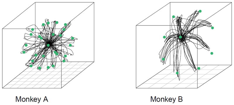
Monkey A: center-out and out-center movement to and from 27 targets on a 3D sphere. Monkey B: center-out movement to eight targets on a 2D circle.

Monkey B

This experiment was conducted in Dr. Aaron Batista’s laboratory at the University of Pittsburgh. A monkey made center-out reaches to eight peripheral targets arranged on a circle and presented in random order, with each target available for repetition only after all targets were acquired successfully. We use 284 successful trials recorded within a single day. Even though the targets were in a 2D plane, the monkey’s arm was free to move in all directions and the arm position was recorded in 3D using a red LED (PhaseSpace Inc.). We predict the full 3D trajectory of the arm. The neural activity was recorded on a 96-electrode Utah array (Blackrock Microsystems) implanted in the proximal arm region of M1.

Electrode voltage thresholds

The choice of thresholds is a critical component in determining the extent of the information one can observe from the noise. In our experiments, thresholds were set independently on each electrode according to standard procedures within the BCI community, and kept constant for the duration of the experiments. For Monkey A, they were set by an expert to maximize the ability to perform spike-sorting according to his judgement. Overall, the electrode voltages crossed the thresholds at rates between 15 and 140 Hz. Fig.2 shows these rates plotted against the thresholds; they decrease on average as thresholds increase, when less noise and hash might be recorded. For Monkey B, thresholds were set systematically at 3 SDs below the means of the bandpass filtered voltage traces. The plot of rates versus thresholds shows no clear trend, which is reasonable since thresholds were set according to a fixed criterion. Overall, the voltages crossed the thresholds at rates between 10 and 50 Hz, i.e. less frequently than for monkey A, which suggests that the relatively large 3 SDs thresholds discarded more noise, or the signal to noise ratio was better.

Figure 2.

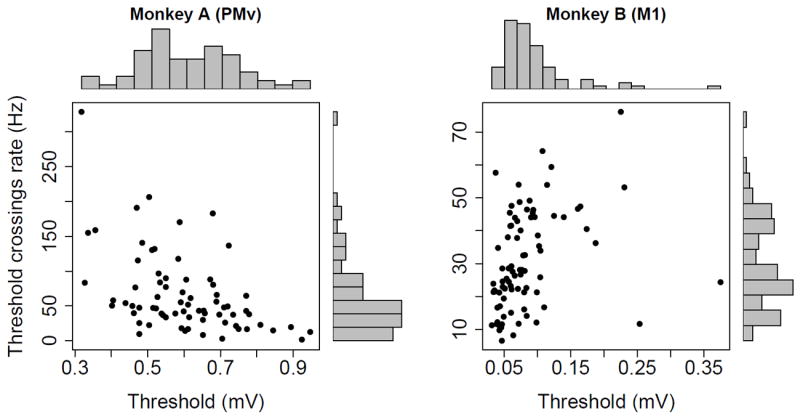
Electrode voltage thresholds versus threshold crossings rates for both monkeys. Each point corresponds to an electrode.

2.2. Decoding from single-unit activity

Let v_t denote the 3-dimensional arm velocity at time t, and ${\mathbf{s}}_t={\left(s_t^1,s_t^2,\dots ,s_t^N\right)}^T,$ the vector of spike counts in time bin t for N putative neurons. Two broad classes of decoding methods exist: one, reverse regression, predicts v directly as a function of s; the other relies on physiological models of firing rates as functions of kinematics. We use the latter, and model the firing rates as linear functions of velocity:

$${\mathbf{s}}_t={\beta }_{\mathbf{0}}+\mathbf{B}{\mathbf{v}}_{t-\tau }+{\eta }_t,$$ (1)

where B is the N × 3 matrix of tuning curves coefficients, and η_t is an N-dimensional Gaussian vector with zero mean and variance ${\sigma }_j^2$ for neuron j = 1, 2, …, N; we assume that neurons are independent. We use spike counts in 16ms bins lagged τ = 130ms for monkey A, and 32ms bins lagged τ = 64ms for monkey B, where τ was chosen to achieve the highest R² in eq.1. We decode using two standard algorithms: the optimal linear estimator (OLE, Salinas & Abbot 1994, Chase et al. 2009), and the Kalman filter (Wu et al. 2006). OLE consists of estimating v_t in eq.1 by maximum likelihood. Kalman filtering supplements eq.1 with a state equation that models the smoothness of arm trajectories; we use the random walk model:

$${\mathbf{v}}_t=\mathbf{A}{\mathbf{v}}_{t-1}+{\epsilon }_t,$$ (2)

where A is a 3 × 3 matrix and ε_t is Gaussian noise. Eq.2 serves as a prior model for eq.1, and the decoded velocity v̂_t is the mean of the posterior distribution of v_t given the spike counts up to time t. Eqs.2 and 1 are estimated using a training dataset, and the decoders performances assessed on separate testing datasets; details are in sec.3.

2.3. Spike-sorting methods

We now describe the different spike counts s_t we use as inputs to the decoders. Figure 3 shows where these fit in the taxonomy of spike-sorting schemes for extracellular electrode recordings.

Figure 3.

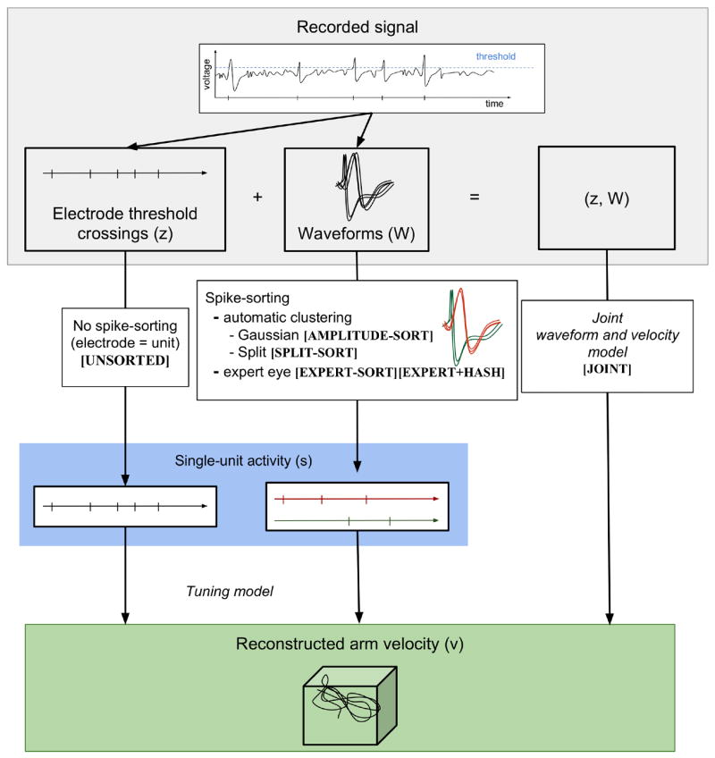
Decoding arm trajectory from extracellular electrode recordings. The recorded signal consists of electrode threshold crossings and waveforms. Decoding directly from threshold crossings does not require spike-sorting. Traditional spikesorting consists of clustering the waveforms (traditionally Gaussian clustering). Split spike-sorting simplifies the clustering to deterministic assignment to disjoint predefined clusters. The joint waveform and velocity model performs spike-sorting and tuning curve estimation in parallel. The names of the specific implementations of each spike-sorting method are marked in square brackets.

UNSORTED

We ignore the waveform measurements and treat the voltage threshold crossings of each electrode as a single putative neuron. Letting $Z_t^j$ be the number of threshold crossings on electrode j in time bin t, then s_t = z_t in eq.1.

EXPERT-SORT

A trained expert identifies unique waveform templates and assigns recorded spikes to single units based on their similarity to each template. Waveforms that do not match any template, the “hash”, are discarded. The number of threshold crossings of electrode j is thus decomposed as the sum of K_j individual neuron spike counts, $y_t^{j,k}$, plus the number of unclassified threshhold crossings, $e_t^j$. The vector of single-unit spike counts in eq.1 contains all neuron spike counts on all electrodes:

$${\mathbf{s}}_t={(y_t^{1,1},y_t^{1,2},\dots ,y_t^{1,K_1},y_t^{2,1},\dots ,y_t^{N,K_N})}^T,$$ (3)

and the hash is discarded. The expert sorting we use in this paper was conducted at the lab where each experiment took place.

EXPERT+HASH

The hash may contain some information for decoding. To test this hypothesis, we decode from the single-unit spike counts (eq.3), augmented by the unclassified threshold crossings on each electrode, $e_t^j$, j = 1, …, N.

MODEL-SORT

The waveforms on electrode j are reduced to p features, a, which are assumed to have the mixture distribution

$$f_j(a)=\sum _{i=1}^{K_j}{\pi }_{j,i}{f}_{j,i}(a),$$ (4)

where K_j is the number of neurons, π_j,i is the proportion of spikes from neuron i, and f_j,i is the distribution of their features, which we assume is p-dimensional Gaussian (Lewicki 1998). Under this model, the spike count for unit k on electrode j in time bin t (eq.3) is

$$y_t^{j,k}=\sum _{m=1}^{M_j}\left(\frac{{\pi }_{j,k}{f}_{j,k}(a_t^{j,m})}{{\sum }_{i=1}^{K_j}{\pi }_{j,i}{f}_{j,i}(a_t^{j,m})}\right),$$ (5)

where $a_t^{j,1}$, $a_t^{j,2},\dots ,a_t^{j,M_j}$ are the features of the M_j spikes recorded in bin t for electrode j. Eq.5 uses soft clustering, so the number of spikes assigned to a neuron can take non-integer values (Ventura 2009b).

An expectation maximization (EM) algorithm is often used to estimate eq.4. This algorithm is very sensitive to initial values, and often converges to local maxima of the likelihood. This impacts greatly the accuracy of spike-sorting, and may in turn impact decoding efficiency. We considered three implementations with careful choices of initial values. The first is an expert sorter: we reduced the waveforms to their first three principal components (PCs), which we plotted to determine carefully the number K_j of clusters, as well as their centers and variances. We used these clusters, plus a clutter cluster to collect the hash, as initial values to fit eq.4. Decoding from the resulting single-unit spike counts (eq.5) gave results that were never better than EXPERT+HASH decoding, so we do not report them in sec.3. We also consider two faster and fully automatic implementations of MODEL-SORT: AMPLITUDE-SORT and SPLIT-SORT.

AMPLITUDE-SORT

To minimize computation, we reduce the spike waveforms to single features, their amplitudes, which we assume have the distribution in eq.4 with f_j,i univariate Gaussians. We obtain the single-units spike counts (eq.3) per eq.5. We also eliminate manual intervention by using automatic initial values to fit eq.4. In particular, we center the initial f_i,j at K_i points equally spaced over the range of the training amplitude data, a sensible option in 1D. Full details are in sec.2.4

SPLIT-SORT

We model the waveform amplitudes according to eq.4, as above, but we let f_j,i to be non-overlapping contiguous uniform distributions with support(ω_j,i−1, ω_j,i]. We do not fit eq.4 by EM, but take w_j,i to be the i(100/K_j)th observed percentile of the amplitudes in a training set for electrode j, and π_j,i be 1/K_j for all i. That is, we form equal-sized clusters simply by binning the observed waveform amplitudes, as illustrated in figure 4. We did, however, estimate the number of mixture components K_j : we decoded all test sets for K_j = K ranging from 1 to 10 on all electrodes; decoding improved as K increased from 1 to 4, then stabilized. We also used different K_j ’s to form equal-sized clusters across electrodes, with no further improvement. We therefore settled for K = K_j = 4 for all electrodes. The single-unit spike count for unit k on electrode j in time bin t, $y_t^{j,k}$ in eq.3, is the number of spikes in bin t that have amplitudes in (ω_j,k−1, ω_j,k].

Figure 4.

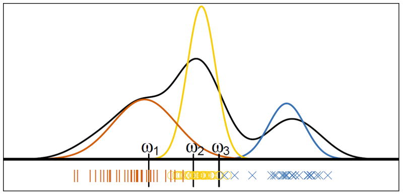
Split-sorting a simulated electrode. The red, yellow, and blue curves are the waveform amplitude distributions of three neurons. The black curve is their mixture, from which we simulated 100 amplitudes, marked on the x-axis with ∣, ○ and ×; the symbols and colors indicate from which mixture components the values were sampled. The vertical lines at ω₁, ω₂ and ω₃ mark the cluster boundaries for split spike-sorting, assuming we want K = 4 clusters.

The advantage of split-sorting is its simplicity, a drawback that it is not designed to isolate neurons well, although it may still perform well: in figure 4, the three neurons have waveform amplitudes whose distributions overlap little, so that the K = 4 splitsorting clusters are comprised almost entirely of observations from single neurons. Note also that isolating neurons perfectly may not translate into greatly improved decoding.

2.4. Decoding using a joint waveform and velocity observation equation (JOINT)

Traditional spike-sorting algorithms use waveforms to assign spikes to neurons. Ventura (2009a) pointed out that when tuning curves are modulated by kinematics, they too contain information about neurons’ identities, and proposed a waveform model that combines the two sources of spike identity information:

$$f_j(a\mid \mathbf{v})=\sum _{i=1}^{K_j}{\pi }_{j,i}(\mathbf{v})f_{j,i}(a),$$ (6)

where ${\pi }_{j,i}(\mathbf{v})=g_{j,i}(\mathbf{v})/\left({\sum }_{k=1}^{K_j}{g}_{j,k}(\mathbf{v})\right)$ is the proportion of spikes from neuron i on electrode j at velocity v, and g_j,i(v) is the tuning curve of neuron i on electrode j. The waveform model (eq.4) on which traditional spike-sorting relies is equal to eq.6 when all tuning curves are constant or equal to each other, for then π_j,i(v) = π_j,i for all v. But eq.4 is a poor approximation of eq.6 when the π_j,i’s are highly modulated by v, in which case we might expect more accurate decoding from eq.6.

Single-unit spike counts (eq.3) could be calculated per eq.5 with π_j,i replaced by π_j,i(v_t), but they cannot be used for decoding because they depend on the very kinematics v_t we seek to predict. Ventura (2009a) circumvented that problem by plugging the decoded velocity at time t − 1 as a proxy for v_t, and used OLE decoding. Here, we bypass spike-sorting and decode v_t directly from the joint distribution of the electrodes’ spike counts and their waveforms; i.e. we use as the observation equation the product of the conditional waveform distributions (eq.6, j = 1, … N) and the electrodes’ spike counts distributions (eq.1 with s_t equal to the UNSORTED spike counts z_t). We cannot decode via OLE or Kalman filtering because eq.6 is not linear in velocity. Instead, we obtain the maximum likelihood (ML) estimator of v_t numerically, and use a particle filter (Brockwell et al. 2004) to obtain its posterior mean.

To fit eq.6, we use the EM algorithm in Ventura (2009a). To minimize computation and eliminate manual intervention, we mirror our approach for AMPLITUDE-SORT: we reduce the waveforms to their amplitudes and choose initial values automatically. We let the f_j.i have initial means at K_j points equally spaced over the range of the training amplitude data, initial variances be equal to their sample variance, initial mixing proportions be constant and equal, and K_j be chosen using the Bayesian information criterion (Schwartz 1978), allowing up to K_j = 5 units per electrode. Recall that AMPLITUDE-SORT models the waveforms per eq.6 with mixing proportions held constant, i.e. π_j,i(v) = π_j,i. To assess the effect of using constant versus variable π_j,i’s on decoding, without it being confounded with potentially different solutions of the EM algorithm, we use the fit of eq.6 for AMPLITUDE-SORT, replacing the π_j,i(v) by their integrals over the kinematics v in the training set.

3. Results

We compare the performances of the decoders considered here using data from the two experiments described in sec.2.1 and figure 1. The decoders take as input spikes sorted according to the methods summarized in table 1. Figure 5 shows the number of units identified by each spike-sorter. For UNSORTED, the electrode arrays of monkeys A and B have 73 and 83 active electrodes respectively. For EXPERT-SORT, the experts could classify reliably 20% and 50% of all threshold crossing events from all electrodes, resulting in a total of 71 and 86 well-isolated units for monkeys A and B; the reason for the small 20% is because the electrode thresholds for monkey A were more permissive, as addressed in sec.2.1. EXPERT+HASH uses the units identified by EXPERT-SORT, plus one extra hash unit per electrode. SPLIT-SORT produced the largest number of units (284 and 332), followed by AMPLITUDE-SORT (181 and 225). Note that no threshold crossings are discarded, except with EXPERT-SORT, which retains only the well-isolated units.

Table 1.

Spike-sorting methods

Name	Method
UNSORTED	No sorting: we treat the voltage threshold crossings of each electrode as a single putative neuron.
EXPERT-SORT	An expert identifies well-isolated units by clustering waveforms visually, and discards the hash.
EXPERT+HASH	EXPERT-SORT, but with the hash retained as an extra unit on each electrode.
AMPLITUDE-SORT	Waveform amplitudes are clustered using a mixture of Gaussians, using automatic initial values.
SPLIT-SORT	Amplitudes are assigned to Uniform clusters that have boundaries at the quartiles of a training set of amplitudes.
JOINT	No sorting: we decode from the joint distribution of electrode spike counts and waveform amplitudes.

Figure 5.

Number of units extracted by each spike-sorting method.

We analyze 1040 trials from Monkey A (five sessions in each of four days; one session consists of 52 unique reaches) and 284 trials from Monkey B, recorded the same day. We only analyze the portion of the trials between movement onset and target acquisition. For monkey B, we do not analyze the return to center portion of the reach, since the animals could be distracted and drinking. Each trial averages 462 and 951 ms between the movement onset and the target acquisition, which amounts to a total of 8 and 4.5 minutes of decoding data for monkeys A and B respectively.

To decode, we assume that units (electrodes or neurons) are independent, and their tuning curves (eq.1) linear in velocity. Spikes are binned and lagged with velocity at the same lag for all units; we use 16msec bins at a 130msec lag for monkey A, and 32msec bins at a 64msec lag for monkey B. These values were chosen to achieve the highest total R² in eq.1. For Monkey A, we use all combinations of four sessions recorded the same day (208 trials) to train the observation and state equations (eqs.1 and 2), and we decode the 52 reaches of the remaining session of that day, totaling 5 × 4 × 52 = 1040 test trials. For monkey B we randomly select 184 trials to train eqs.1 and 2, and we decode the 100 remaining trials. We perform the random trial selection only once. We initialize the decoders at the observed initial velocity for each trial.

We measure the quality of a decoded reach by its root mean squared error (RMSE), i.e. the Euclidean distance between the observed and the decoded velocity trajectories. The relative efficiency of two decoding algorithms is the ratio of the mean squared errors (MSE) of the respective decoded velocity trajectories. If decoders 1 and 2 have MSE ratio r = MSE₁/MSE₂, we calculate the efficiency gain of decoder 2 compared to decoder 1 in percent as (r − 1) * 100 when r > 1, and (1 − 1/r) * 100 when r < 1. Figures 6, 7, and 8 summarize the distributions of efficiency gains for all test trials using box plots, and table 2 contains the median per-trial RMSE of each decoding method. Table 2 suggests that (i) discarding the hash systematically degrades decoding, (ii) decoding without spike-sorting is less efficient than decoding from spike-sorted data, and (iii) all spike-sorting schemes yield comparable decoding efficiencies. Therefore, we should not discard spikes, we should spike-sort, and using an easy spike-sorting scheme is as good as any. We discuss these points further in the next subsections.

Figure 6.

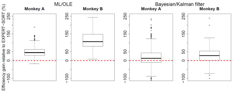
Relative efficiency gain of EXPERT+HASH compared to EXPERT-SORT using ML/OLE and Bayesian/Kalman filter decoding.

Figure 7.

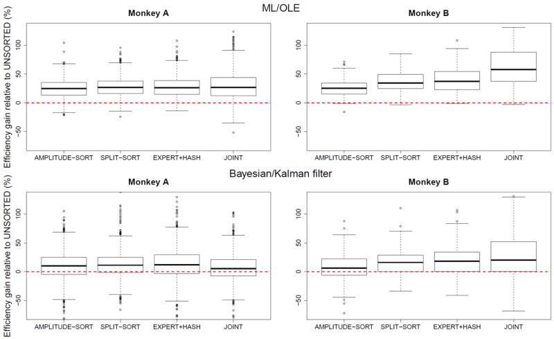
Relative efficiency gain of AMPLITUDE-SORT, SPLIT-SORT, EXPERT+HASH, and JOINT decoding compared to UNSORTED using ML/OLE decoding and Bayesian/Kalman filtering.

Figure 8.

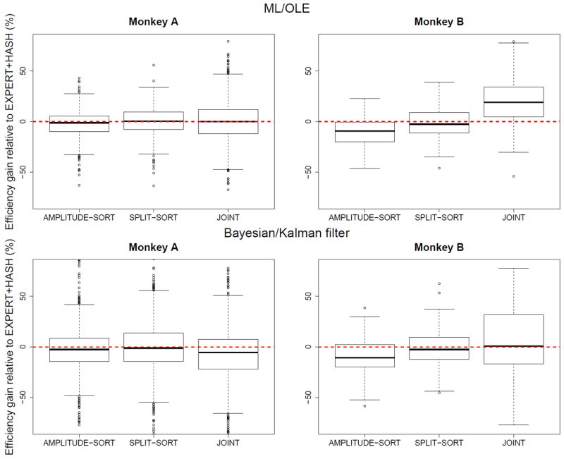
Relative efficiency gain of AMPLITUDE-SORT, SPLIT-SORT, and JOINT decoding compared to EXPERT+HASH using ML/OLE and Bayesian/Kalman filter decoding.

Table 2.

Decoding efficiencies measured by the median over all test trials of the root mean squared error (RMSE), ± one standard deviation. The methods in each panel are sorted by RMSE from the least to the most accurate.

	Method	RMSE (m/sec)
MONKEY A ML/OLE	EXPERT-SORT	0.189±0.021
	UNSORTED	0.176±0.023
	AMPLITUDE-SORT	0.157±0.023
	EXPERT+HASH	0.157±0.021
	SPLIT-SORT	0.156±0.022
	JOINT	0.156±0.022
Bayesian/Kalman filter	EXPERT-SORT	0.087±0.026
	UNSORTED	0.086±0.026
	JOINT	0.084±0.026
	AMPLITUDE-SORT	0.083±0.024
	EXPERT+HASH	0.082±0.024
	SPLIT-SORT	0.082±0.025
MONKEY B ML/OLE	EXPERT-SORT	0.311±0.032
	UNSORTED	0.255±0.023
	AMPLITUDE-SORT	0.228±0.018
	SPLIT-SORT	0.219±0.018
	EXPERT+HASH	0.218±0.017
	JOINT	0.199±0.017
Bayesian/Kalman filter	EXPERT-SORT	0.142±0.040
	UNSORTED	0.139±0.036
	AMPLITUDE-SORT	0.136±0.033
	SPLIT-SORT	0.130±0.034
	JOINT	0.130±0.032
	EXPERT+HASH	0.128±0.033

3.1. Discarding the noise degrades decoding

Expert sorting discards the threshold crossings that could not reliably be classified as belonging to a single unit; there were 80% such crossings for monkey A and 50% for monkey B. Table 2 shows that decoding only with expert-sorted units yields the worst median decoding performance. For 63% of the trials across the two monkeys, it is more efficient to decode from the unsorted electrodes’ threshold crossings than from expertly sorted neurons. When we include the discarded spikes as a separate hash unit on each electrode, the decoding efficiency is comparable to the other decoders (table 2, EXPERT+HASH row). Figure 6 shows the distributions of efficiency gains of EXPERT+HASH compared to EXPERT-SORT. The former is more efficient across decoding methods and monkeys. The improvement is greater for monkey B, which means that the hash contains more information for that monkey. This could be due to at least two factors: (1) the electrode thresholds were chosen differently in the two experiments, which affects the amount of recorded noise, and (2) different experts sorted the spikes from each experiment.

3.2. Spike-sorting improves decoding efficiency

Table 2 shows that, in median, decoding from unsorted spikes is inferior to decoding from sorted spikes. The full distributions of efficiency gains (figure 7) confirm this. For monkey A, all sorting schemes provide comparable efficiency gains (25 – 27% under ML/OLE decoding, and 5– 12% under Bayesian/Kalman filtering) compared to UNSORTED. For monkey B, sorting based on amplitude yields the least improvement (25% under ML/OLE and 6% under Bayesian/Kalman filtering), and the joint model yields the greatest (58% under ML/OLE and 20% under Bayesian/Kalman filtering). The joint model provides lesser improvements for monkey A, which we discuss further in Section 3.4.

3.3. Crude sorting is as effective for decoding as accurate spike-sorting

The relative efficiencies of all methods compared to EXPERT+HASH (figure 8) suggest that AMPLITUDE-SORT decoding is the least efficient of all sorting methods (this excludes the joint model). Furthermore, the crude SPLIT-SORT procedure yields efficiencies comparable to the time consuming expert sorting, which suggests that, for the purpose of decoding, a sub-optimal spike-sorter is competitive compared to expert or model-based spike-sorting. SPLIT-SORT creates artificial neurons that are composed of one or more, full or partial, real neurons. If the real neurons have different tuning curves and different waveform amplitude distributions, then the artificial neurons also have different tuning curves, and perhaps this is what matters most for decoding. If the real neurons on an electrode have the same tuning curves, or the same waveform distributions, in which case spikes cannot be sorted, then the artificial neurons also have the same tuning curves, which preserves the information about velocity provided by the electrode. Note that the good performance of SPLIT-SORT is not due to the larger number of artificial neurons it creates, otherwise splitting each electrode in ever larger numbers of artificial neurons would ameliorate decoding many-folds. In the two datasets analyzed here, K = 4 fixed clusters per electrode worked best; using smaller K’s degraded decoding, and larger K’s did not improve it.

3.4. Decoding using the joint model is not uniformly superior

The joint waveform and velocity model (eq. 6) contains all the information about the kinematics so it should in principle outperform the other methods. Figure 8 suggests it is not always the case in practice: JOINT decoding yields no improvement for monkey A compared to AMPLITUDE-SORT, SPLIT-SORT or EXPERT+HASH under either ML or Bayesian decoding. For monkey B, the median improvements are 30% over AMPLITUDE-SORT for ML decoding, and 11% for Bayesian decoding. This suggests that the performance of JOINT decoding depends on the dataset, and that improvements are not guaranteed. As mentioned in section 2.4, JOINT and AMPLITUDE-SORT decoding rely on waveform models that differ only in the unit proportions: the π_k are constant in eq.4 and they are functions of velocity in eq.6. The more modulated the π_k(v_t) are, the more information about velocity eq.6 contains compared to eq.4, and therefore the better JOINT decoding might be. We summarize the modulation in π_k(v_t) by its range across values of v_t. Figure 9 shows the distribution of these ranges across all neurons: the π_k(v_t) are more modulated for monkey B, which likely explains why JOINT decoding is more efficient for monkey B than for monkey A.

Figure 9.

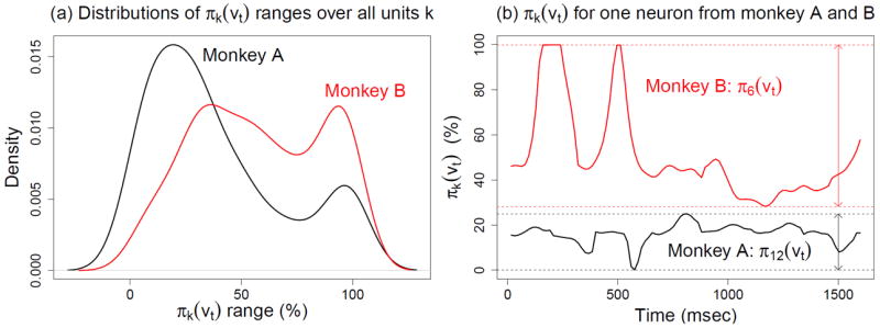
(a) Density of range_k = max_t π_k (v_t) − min_t π_k (v_t) for all neurons k. (b) Sample values for a single unit proportion π_k(v_t) each from monkeys A and B. The function π₆ (v_t) in monkey B fluctuates more than the function π₁₂ (v_t) in monkey A. This relationship holds generally across the neurons of the two monkeys, which contributes to the better performance of JOINT decoding for monkey B.

4. Discussion

We investigated how fast, simple, and fully automatic spike-sorting affects the quality of arm reaching movement reconstructions. Perhaps surprisingly, we find that the two most commonly used methods for performing real-time neural prosthetic control yield the lowest decoding performances in our analysis: (i) decoding using only well-isolated neurons and discarding hash is less efficient than decoding directly from threshold crossings; (ii) if no spike is discarded, decoding from sorted spikes is more efficient than decoding from threshold crossings. In short, the best approach is to spike-sort, but keep the hash. Moreover, the simplistic scheme of sorting by splitting waveform amplitudes into predefined bins performed as well as expert sorting and in some cases outperformed the traditional model-based Gaussian clustering. This suggests that crude automatic spike-sorting yields efficient decoding at minimal computational cost. Interestingly, the benefit of sorting is greater under OLE decoding than Kalman filtering, possibly because the smoothing induced by the state space model mitigates the differences in input signal.

4.1. Information in the hash

The least efficient decoding method was EXPERT decoding, the only method that discards waveform events that do not match well-identified templates. This suggests that there is velocity information in the hash. This is consistent with Fraser et al. (2009) and other studies; e.g. Stark & Abeles (2007) find that multiunit activity can provide more accurate prediction of upcoming movement than the activity of wellisolated single units; Kloosterman et al. (2014) use a dataset in which only 6 – 21% of all spikes are attributable to well-isolated single units, and report that including the hash greatly improves decoding. It remains a topic for future work to discover precisely how much information the noisy waveforms contain, and develop algorithms to extract that information effectively.

This finding may not generalize to closed-loop decoding. Indeed in that context, Fraser et al. (2009) found that on-line prosthetic control using EXPERT decoding, which discards poorly isolated spikes, was as accurate as decoding from threshold crossings. It is possible that in closed-loop, subjects can adapt to the decoder, thus mitigating accuracy differences (Chase et al. 2009).

4.2. Computational overhead

To decode, we assumed that all units were independent, and we fixed every unit’s temporal lag with respect to the kinematic variables to the mean estimated lag. These choices were made for ease of clinical implementation rather than to optimize the accuracies of sorting or decoding. Indeed it is known that using unit correlations and different lags can improve decoding (Wu et al. 2006). We assumed normally distributed spike counts, and linear observation and state equations, because they provide velocity predictions in closed-form, which is computationally efficient. These predictions are also statistically optimal when the assumptions are correct (Kass et al. 2005). However, spike counts have Poisson or Poisson-like distributions, so general point process models (Barbieri et al. 2004) would be more appropriate. We did not consider non-Gaussian models because Bayesian dynamic predictions would require computationally intensive numerical or stochastic optimizations (Brockwell et al. 2004, Koyama et al. 2010). Although we didn’t test these algorithms, we do not think our main findings would change.

The automatic spike-sorting schemes we used were designed to be easy to implement, fast to compute, and require little data manipulation. For both fully automated algorithms we reduced the waveforms to single features, their peak-to-trough waveform amplitudes. For AMPLITUDE sorting, we used automated starting values and greedy model selection in the EM clustering algorithm. The SPLIT sorting procedure was yet simpler, since we fixed the number of units per electrode to four and sorted based solely on the quartiles of the waveform amplitudes in a training dataset. Despite these simplifications, both automated sorting procedures performed as well as expert manual sorting, provided that no spikes were discarded. The performance of SPLIT sorting shows that crude automatic methods can improve decoding efficiency without accurately classifying single-neuron activity. Other than its simplicity, other attractive properties of this method include producing clusters large enough to reliably fit tuning curve models and localized enough to capture single-unit activity, requiring minimal computation and data storage, and trivial fitting to training data; it could also easily be extended to sort higher-dimensional waveform features. Additionally, the SPLIT clusters can trivially be updated on a regular basis to capture possible changes in the waveform distributions due, for example, to electrodes shifting (Calabrese & Paninski 2010) or neurons dying.

State-of-the-art spike-sorters such as template matching algorithms (Quiroga et al. 2004, Rutishauser et al. 2006, Carlson et al. 2014) or wavelet features clustering (Hulata et al. 2002, Brychta et al. 2007) may outperform the ones we tested, but we did not consider them because they are computationally demanding and require expert manual tuning. While the optimal balance of computation overhead and accuracy will likely depend on the specific decoding task and signal quality, the finding that SPLIT sorting performs as well as EXPERT+HASH manual sorting suggests that large improvements in decoding efficiency are unlikely to arise from more accurate waveformbased spike-sorting, at least for these relatively low-dimensional tasks. We also believe our main results, that discarding hash is a bad idea, and that sorting is better than not sorting, will hold true for all reasonable sorting algorithms.

4.3. Decoding from the joint waveform and velocity model

At the other end of the complexity spectrum, JOINT decoding should be statistically optimal, since the model on which it relies contains all the kinematic information. In practice, its performance was mixed, providing improvements only for monkey B using ML decoding, with a 19% median improvement over EXPERT+HASH decoding. We obtained no improvement for Monkey B with Bayesian filtering, or for Monkey A altogether. We speculated, and provided some evidence, that JOINT ML decoding performs better than AMPLITUDE-SORT decoding when tuning curves are highly modulated with velocity.

Kloosterman et al. (2014) also decode from a joint model that they fit to data nonparametrically. They report a 14% mean improvement of JOINT ML decoding compared to ML decoding from well-isolated units with hash, to reconstruct 1D trajectories from rat hippocampal data. The relevant comparison using our nomenclature is between JOINT and EXPERT+HASH, and the improvement of JOINT decoding is comparable across studies: their 14% to our 19%. They do not report results for Bayesian dynamic decoding. Our initial conclusion is that both the JOINT decoding approaches reported here and there are too computationally intensive to be implemented in the lab or the clinic, especially since they appear to provide only modest, if any, improvements. Some modifications permitting OLE decoding, as in Ventura (2009a), or Kalman filtering would at least make its implementation more attractive.

4.4. Generalizability

Our results were obtained on data collected from two different monkeys in two different labs, each with their own training protocols and experimental equipment. We analyzed a total of 1040 3D trials from Monkey A and 284 2D trials from Monkey B, and the results hold up independently for each. Further, our results are entirely in keeping with the previous studies cited above. Additionally, Kloosterman et al. (2014) report similar results on 12 different data sets from rat hippocampus tetrode recordings. In particular, they find that there is information for decoding in the hash, that careful manual spikesorting can perform as well as completely automatic spike-sorting for the purpose of decoding, and that decoding from the joint model does not always perform better than decoding from spike-sorted counts. They also show that accurate spike-sorting is not crucial for decoding performance, namely, they report an example in which automatic clustering produced better decoding results before the expert cluster refinement.

However, an important aspect is the choice of electrode crossing thresholds. It is likely that different choices of thresholds might re-balance the relative efficiencies of sorting and decoding methods. A thorough analysis of the effect of threshold choice on decoding performance, while interesting, is beyond the scope of this paper.

4.5. Robustness versus accuracy

This study does not control for possible data non-stationarities. Changes in the tuning properties of the recorded signal from the training to the testing session could degrade the performance of the decoder. The electrodes can also shift, which changes the distribution of the recorded waveforms (Calabrese & Paninski 2010). The effect of such non-stationarity might be different across decoders and sorting methodology; some sorting methods may be more robust to waveform or tuning changes than others. Nevertheless, the case that we make is most likely applicable to adaptable models as well. Future attempts to improve the absolute performance of any of the decoders discussed here could address robustness using auto-adaptive decoding algorithms (Orsborn et al. 2012, Li et al. 2011, Zhang & Chase 2013). Note also that the SPLIT clusters can be updated regularly at no computational cost, to track potential waveform changes.

References

- Barbieri R, Frank LM, Nguyen DP, Quirk MC, Solo VC, Wilson MA, Brown EN. Neural Comput. 2004;16(2):277–307. doi: 10.1162/089976604322742038. URL: http://dx.doi.org/10.1162/089976604322742038. [DOI] [PubMed] [Google Scholar]
- Brockwell AE, Rojas AL, Kass RE. J Neurophysiol. 2004;91(1):1899–1907. doi: 10.1152/jn.00438.2003. URL: http://www.ncbi.nlm.nih.gov/pubmed/15010499?dopt=Abstract. [DOI] [PubMed] [Google Scholar]
- Brychta RJ, Tuntrakool S, Appalsamy M, Keller NR, Robertson D, Shiavi RG, Diedrich A. Biomedical Engineering, IEEE Transactions on. 2007;54(1):82–93. doi: 10.1109/TBME.2006.883830. [DOI] [PMC free article] [PubMed] [Google Scholar]
- Calabrese A, Paninski L. J Neurosci Meth. 2010 URL: http://www.ncbi.nlm.nih.gov/pubmed/21182868.
- Carlson D, Vogelstein J, Wu Q, Lian W, Zhou M, Stoetzner C, Kipke D, Weber D, Dunson D, Carin L. Biomedical Engineering IEEE Transactions on. 2014;61(1):41–54. doi: 10.1109/TBME.2013.2275751. [DOI] [PubMed] [Google Scholar]
- Carmena JM, Lebedev MA, Crist RE, O’Doherty JE, Santucci DM, Dimitrov DF, Patil PG, Henriquez CS, Nicolelis MaL. PLoS biology. 2003;1(2):E42. doi: 10.1371/journal.pbio.0000042. URL: http://www.pubmedcentral.nih.gov/articlerender.fcgi?artid=261882. [DOI] [PMC free article] [PubMed] [Google Scholar]
- Chase SM, Schwartz AB, Kass RE. Neural networks : the official journal of the International Neural Network Society. 2009;22(9):1203–13. doi: 10.1016/j.neunet.2009.05.005. URL: http://www.pubmedcentral.nih.gov/articlerender.fcgi?artid=2783655. [DOI] [PMC free article] [PubMed] [Google Scholar]
- Chestek CA, Gilja V, Nuyujukian P, Foster JD, Fan JM, Kaufman MT, Churchland MM, Rivera-Alvidrez Z, Cunningham JP, Ryu SI, Shenoy KV. Journal of Neural Engineering. 2011;8(4):045005. doi: 10.1088/1741-2560/8/4/045005. URL: http://stacks.iop.org/1741-2552/8/i=4/a=045005. [DOI] [PMC free article] [PubMed] [Google Scholar]
- Collinger JL, Wodlinger B, Downey JE, Wang W, Tyler-Kabara EC, Weber DJ, McMorland AJC, Velliste M, Boninger ML, Schwartz AB. Lancet. 2013;381(9866):557–64. doi: 10.1016/S0140-6736(12)61816-9. URL: http://www.ncbi.nlm.nih.gov/pubmed/23253623. [DOI] [PMC free article] [PubMed] [Google Scholar]
- Fraser GW, Chase SM, Whitford A, Schwartz AB. J Neural Eng. 2009;6(5):055004. doi: 10.1088/1741-2560/6/5/055004. URL: http://www.ncbi.nlm.nih.gov/pubmed/19721186. [DOI] [PubMed] [Google Scholar]
- Fraser GW, Schwartz AB. J Neurophysiology. 2012;107(7):1970–8. doi: 10.1152/jn.01012.2010. URL: http://www.pubmedcentral.nih.gov/articlerender.fcgi?artid=3331662. [DOI] [PMC free article] [PubMed] [Google Scholar]
- Ge D, Farina D. John Wiley and Sons Inc; 2013. pp. 155–172. URL: http://dx.doi.org/10.1002/9781118628522.ch8. [Google Scholar]
- Gibson S, Judy JW, Markovi D. IEEE Signal Process Mag. 2012;29(1):124–143. URL: http://lifesciences.ieee.org/images/pdf/2012-01-spike.pdf. [Google Scholar]
- Gilja V, Nuyujukian P, Chestek C, Cunningham JP, Yu BM, Fan JM, Churchland MM, Kaufman MT, Kao JC, Ryu SI, Shenoy KV. Nature neuroscience. 2012;15(12):1752–7. doi: 10.1038/nn.3265. URL: http://www.pubmedcentral.nih.gov/articlerender.fcgi?artid=3638087. [DOI] [PMC free article] [PubMed] [Google Scholar]
- Harris KD, Henze Da, Csicsvari J, Hirase H, Buzs′aki G. J Neurophysiology. 2000;84(1):401–14. doi: 10.1152/jn.2000.84.1.401. URL: http://www.ncbi.nlm.nih.gov/pubmed/10899214. [DOI] [PubMed] [Google Scholar]
- Hochberg LR, Bacher D, Jarosiewicz B, Masse NY, Simeral JD, Vogel J, Haddadin S, Liu J, Cash SS, van der Smagt P, Donoghue JP. Nature. 2012;485(7398):372–5. doi: 10.1038/nature11076. URL: http://www.pubmedcentral.nih.gov/articlerender.fcgi?artid=3640850. [DOI] [PMC free article] [PubMed] [Google Scholar]
- Hochberg LR, Serruya MD, Friehs GM, Mukand J, Saleh M, Caplan AH, Branner A, Chen D, Penn RD, Donoghue JP. Nature. 2006;442(7099):164–71. doi: 10.1038/nature04970. URL: http://www.ncbi.nlm.nih.gov/pubmed/16838014. [DOI] [PubMed] [Google Scholar]
- Hulata E, Segev R, Ben-jacob E. J Neurosci Meth. 2002;117:1–12. doi: 10.1016/s0165-0270(02)00032-8. [DOI] [PubMed] [Google Scholar]
- Kass RE, Ventura V, Brown EN. J Neurophysiology. 2005;94(1):8–25. doi: 10.1152/jn.00648.2004. URL: http://jn.physiology.org/content/94/1/8.abstract. [DOI] [PubMed] [Google Scholar]
- Kloosterman F, Layton SP, Chen Z, Wilson Ma. J Neurophysiology. 2014 doi: 10.1152/jn.01046.2012. URL: http://www.ncbi.nlm.nih.gov/pubmed/24089403. [DOI] [PMC free article] [PubMed]
- Koyama S, Castellanos L, Shalizi C, Kass RE. J Am Stat Assoc. 2010;105(489):170–180. doi: 10.1198/jasa.2009.tm08326. URL: http://arxiv.org/abs/1004.3476. [DOI] [PMC free article] [PubMed] [Google Scholar]
- Lewicki MS. Network (Bristol, England) 1998;9(4):R53–78. URL: http://www.ncbi.nlm.nih.gov/pubmed/10221571. [PubMed] [Google Scholar]
- Li Z, Lebedev MA, Nicolelis MAL. Neural Comput. 2011;3204(23):3162–3204. doi: 10.1162/NECO_a_00207. URL: http://www.ncbi.nlm.nih.gov/pubmed/21919788. [DOI] [PMC free article] [PubMed] [Google Scholar]
- Mulliken GH, Musallam S, Andersen RA. J Neurosci. 2008;28(48):12913–12926. doi: 10.1523/JNEUROSCI.1463-08.2008. URL: http://www.ncbi.nlm.nih.gov/pubmed/19036985. [DOI] [PMC free article] [PubMed] [Google Scholar]
- Orsborn AL, Dangi S, Moorman HG, Carmena JM. IEEE Trans Neural Syst Rehabil Eng. 2012;20(4):468–77. doi: 10.1109/TNSRE.2012.2185066. URL: http://www.ncbi.nlm.nih.gov/pubmed/22772374. [DOI] [PubMed] [Google Scholar]
- Quiroga RQ. Scholarpedia. 2007;2(12):3583. revision 137442. [Google Scholar]
- Quiroga RQ, Nadasdy Z, Ben-Shaul Y. Neural computation. 2004;16(8):1661–87. doi: 10.1162/089976604774201631. URL: http://www.ncbi.nlm.nih.gov/pubmed/15228749. [DOI] [PubMed] [Google Scholar]
- Rutishauser U, Schuman EM, Mamelak AN. J Neurosci Meth. 2006;154(1-2):204–24. doi: 10.1016/j.jneumeth.2005.12.033. URL: http://www.ncbi.nlm.nih.gov/pubmed/16488479. [DOI] [PubMed] [Google Scholar]
- Sahani M. PhD thesis. California Institute of Technology Pasadena, CA: USA; 1999. Latent Variable Models for Neural Data Analysis. AAI9932856. URL: http://www.gatsby.ucl.ac.uk/~maneesh/thesis/thesis.double.pdf. [Google Scholar]
- Salinas E, Abbot LF. J Comp Neuroci. 1994;1(1):89–104. URL: http://neurotheory.columbia.edu/larry/SalinasJCompNeuro94.pdf. [Google Scholar]
- Schwartz AB. J Physiology. 2007;579(Pt 3):581–601. doi: 10.1113/jphysiol.2006.126698. URL: http://www.pubmedcentral.nih.gov/articlerender.fcgi?artid=2151362. [DOI] [PMC free article] [PubMed] [Google Scholar]
- Schwartz G. The Annals of Applied Statistics. 1978;6(2):461–464. URL: http://www.jstor.org/stable/2958889. [Google Scholar]
- Serruya M, Hatsopoulos NG, Paninski L, Fellows MR, Donoghue JP. Nature. 2002 Mar;416:141–142. doi: 10.1038/416141a. [DOI] [PubMed] [Google Scholar]
- Stark E, Abeles M. J Neurosci. 2007;27(31):8387–8394. doi: 10.1523/JNEUROSCI.1321-07.2007. URL: http://www.jneurosci.org/content/27/31/8387.abstract. [DOI] [PMC free article] [PubMed] [Google Scholar]
- Suminski AJ, Tkach DC, Fagg AH, Hatsopoulos NG. J Neurosci. 2010;30(50):16777–87. doi: 10.1523/JNEUROSCI.3967-10.2010. URL: http://www.pubmedcentral.nih.gov/articlerender.fcgi?artid=3046069. [DOI] [PMC free article] [PubMed] [Google Scholar]
- Velliste M, Perel S, Spalding MC, Whitford AS, Schwartz AB. Nature. 2008;453(7198):1098–101. doi: 10.1038/nature06996. URL: http://www.ncbi.nlm.nih.gov/pubmed/18509337. [DOI] [PubMed] [Google Scholar]
- Ventura V. Neural Computation. 2008;20(4):923–63. doi: 10.1162/neco.2008.02-07-478. URL: http://www.pubmedcentral.nih.gov/articlerender.fcgi?artid=3124143. [DOI] [PMC free article] [PubMed] [Google Scholar]
- Ventura V. Neural Computation. 2009a;21(9):2466–501. doi: 10.1162/neco.2009.12-07-669. URL: http://www.ncbi.nlm.nih.gov/pubmed/19548802. [DOI] [PMC free article] [PubMed] [Google Scholar]
- Ventura V. PNAS. 2009b;106(17):6921–6. doi: 10.1073/pnas.0901771106. URL: http://www.pubmedcentral.nih.gov/articlerender.fcgi?artid=2678477. [DOI] [PMC free article] [PubMed] [Google Scholar]
- Wu W, Gao Y, Bienenstock E, Donoghue JP, Black MJ. Neural computation. 2006;18(1):80–118. doi: 10.1162/089976606774841585. URL: http://www.ncbi.nlm.nih.gov/pubmed/16354382. [DOI] [PubMed] [Google Scholar]
- Zhang Y, Chase SM. 35th Int. IEEE EMBS Conf.; Osaka, Japan. 2013. Jul, URL: http://ieeexplore.ieee.org/stamp/stamp.jsp?arnumber=06611194. [Google Scholar]