Multisensory decisions provide support for probabilistic number representations

Abstract

A large body of evidence suggests that an approximate number sense allows humans to estimate numerosity in sensory scenes. This ability is widely observed in humans, including those without formal mathematical training. Despite this, many outstanding questions remain about the nature of the numerosity representation in the brain. Specifically, it is not known whether approximate numbers are represented as scalar estimates of numerosity or, alternatively, as probability distributions over numerosity. In the present study, we used a multisensory decision task to distinguish these possibilities. We trained human subjects to decide whether a test stimulus had a larger or smaller numerosity compared with a fixed reference. Depending on the trial, the numerosity was presented as either a sequence of visual flashes or a sequence of auditory tones, or both. To test for a probabilistic representation, we varied the reliability of the stimulus by adding noise to the visual stimuli. In accordance with a probabilistic representation, we observed a significant improvement in multisensory compared with unisensory trials. Furthermore, a trial-by-trial analysis revealed that although individual subjects showed strategic differences in how they leveraged auditory and visual information, all subjects exploited the reliability of unisensory cues. An alternative, nonprobabilistic model, in which subjects combined cues without regard for reliability, was not able to account for these trial-by-trial choices. These findings provide evidence that the brain relies on a probabilistic representation for numerosity decisions.

considerable evidence suggests that animals and humans possess an approximate number sense, believed to be the precursor of complex symbolic manipulations of numbers developed by humans (Dehaene 2011). The approximate number sense allows us to perceive numerosity in sensory scenes even when other cues that might be correlated with number, such as size or surface area, are eliminated (Piazza et al. 2004). Furthermore, evidence suggests that this ability is innate: preverbal babies are capable of estimating numbers as large as 32 (Xu 2003; Xu and Spelke 2000; Xu et al. 2005), and adults in indigenous cultures without mathematical education can represent and manipulate numbers in some circumstances (Pica et al. 2004).

A number of experiments have identified cortical regions that may be necessary for the representation of number. For example, neurons in monkey posterior parietal cortex are sometimes “tuned” for a particular number: they fire maximally for that number and less so for other numbers (Nieder and Dehaene 2009; Nieder and Miller 2004; but see Roitman et al. 2007). Some areas in the human brain are likewise sensitive to numerosity: human parietal areas are activated in numerosity tasks (Chochon et al. 1999; Pinel et al. 2001).

Despite these findings, it is not clear whether the brain uses a scalar or a probabilistic strategy to represent number. If neurons were to represent numbers as scalars (Fig. 1, A and B, right panels in insets), neural circuits would represent one single-value estimate of numerosity on a given trial in response to a stimulus such as the dot display shown in Fig. 1. Naturally, this estimate might differ from trial-to-trial since either sensory noise or a subject's bias might drive the scalar estimate up or down. However, within a trial, only a single number is represented. The disadvantage of a scalar representation is that the reliability of the number estimate is unknown (right panels in insets of Fig. 1, A and B, are the same, although the stimulus is unreliable in Fig. 1B). This is particularly problematic when there are two sources of information, a reliable source and an unreliable source. In this case, the optimal strategy consists of summing the two estimates weighted by their respective reliability (Ernst and Banks 2002; Jacobs 1999). This is intuitive: reliable inputs should have a stronger impact on decisions than unreliable ones. Without access to reliability, subjects cannot apply this optimal strategy but can use a simpler strategy such as selecting one source of information randomly on every trial to guide the choice (we refer to this as the “coin flip” model). Interestingly, scalar representations are commonly used in neural models, particularly models based on attractor dynamics where the dimension of the attractor is equal to the dimension of the encoded variables (Cohen and Grossberg 1983; Deneve et al. 2001; Hopfield 1982; Skaggs et al. 1995; Wang 2009; Wills et al. 2005).

Fig. 1.

Probabilistic vs. scalar representation of numerosity. A: subject estimates numerosity from a reliable (bright) visual stimulus. Inset, left: stimuli lead to a distribution of possible numerosities, peaking near the correct value; right: stimuli lead to a scalar estimate of numerosity. B: subject estimates numerosity from an unreliable (low contrast) visual stimulus. Inset, left: stimuli lead to a distribution of possible numerosities that is much broader than in the corresponding example in A; right: stimuli lead to a scalar estimate of numerosity, similar to the corresponding example in A.

An alternative to a scalar representation is a probabilistic representation (Fig. 1, A and B, left panels in insets). Theories of probabilistic inference in neural circuits describe how probability distributions could be extracted, represented, and used for further inference (for review, see Pouget et al. 2013). For instance, neurons might use probabilistic population codes (Ma et al. 2006) in which the mean of the distribution is encoded by the position of the hill of activity, whereas the variance of the distribution is encoded by the gain, or height, of the hill of activity, with low gain corresponding to higher variance. These representations have the advantage that they automatically encode the reliability associated with the numerosity estimate: unreliable (e.g., low contrast) stimuli would lead to much broader distributions than reliable stimuli (compare left panels in insets of Fig. 1, A and B). Access to stimulus reliability means that subjects are better equipped to use multiple sources of information for decisions. For instance, they could combine sources of information according to their reliability (“optimal model;” Ernst and Banks 2002; Jacobs 1999; van Beers et al. 1996), or they could determine the more reliable source and ignore the other source (referred to as “max model” hereafter). Both strategies are probabilistic in that they require an estimate of stimulus reliability to define how stimuli are used to inform the decision. The two strategies differ in the possible weights that are assigned to each source of information: in an optimal model, weights can take on a range of values, whereas in a max model, weights are either 0 or 1.

The consequence of scalar versus probabilistic representations, as described above, is explicit when multiple sources of information weigh in on the choice. Because most numerosity studies present subjects with a single source of information, the default assumption has been that the brain represents numbers as scalars. Existing experiments have mainly focused on the models' predictions for how noise scales with the number of stimulus objects: a logarithmic mental number line with constant noise (Dehaene and Changeux 1993) versus a linear mental number line with linearly increasing noise (Gallistel and Gelman 1992). These potential noise sources are critical for understanding trial-to-trial fluctuations of number estimate but leave unexamined how numbers are represented on individual trials.

The existence of a probabilistic representation for quantities other than numerosity has been explicitly tested via decisions in which multiple sources of evidence are present. These decisions have exposed probabilistic representations in the neural systems used to estimate depth (Jacobs 1999), limb position (van Beers et al. 1996), surface slant (Knill and Saunders 2003), heading direction (Fetsch et al. 2009), repetition rate (Sheppard et al. 2013), object location (Alais and Burr 2004), and object height (Ernst and Banks 2002). In all cases, experimenters first manipulated the reliability of each source of information, typically by varying the amount of noise added to a stimulus (Fetsch et al. 2009) on every trial or adjusting its intensity (Raposo et al. 2012; Sheppard et al. 2013). Next, they measured whether subjects leveraged that reliability when making multisensory decisions. In many studies, subjects' choices on multisensory trials were influenced by the reliability of each unisensory stimulus, in keeping with a probabilistic representation. Interestingly, similar probabilistic strategies are evident in multiple stimulus contexts (Knill and Saunders 2003; van Beers et al. 1996) and multiple species (Fetsch et al. 2009; Raposo et al. 2012; Sheppard et al. 2013), despite different strategies for manipulating reliability in each study.

The use of multiple sources of information that differ in their reliability is key because it is under these conditions that probabilistic and scalar representations make different predictions. Thus, although previous experiments have shown that bimodal numerosity stimuli can improve behavioral performance (Jordan and Baker 2011; Jordan et al. 2008), these results cannot be taken as conclusive evidence for probabilistic numerosity representations because they used only one level of reliability for each modality.

We used this approach to test for a probabilistic representation of numerosity. We designed a novel multisensory numerosity task and evaluated whether subjects used stimulus reliability to guide decisions. We then considered three models for multisensory integration (the optimal, max, and coin flip models), only two of which take into account reliability (the optimal and max models), and asked which one of these models best accounts for the subjects' performance via Bayesian model comparison. We found that subjects made more precise numerosity judgments when stimuli were multisensory and that they combined the two unisensory cues via a strategy that took into account reliability. These observations support a probabilistic number representation.

METHODS

Behavioral task.

Subjects were trained on a multisensory numerosity task. Each trial consisted of a series of auditory or visual “events” (duration: 1 frame = 10 ms) embedded in background noise of constant amplitude. Visual events were flashes of light, and auditory events were brief tones. Next, the following procedure was undertaken to prevent subjects from performing the task solely on the basis of nonnumeric stimulus attributes such as event rate or total duration (Fig. 2). After selecting numerosity (Fig. 2A), we sampled the desired mean interevent interval time of a given trial from a uniform distribution between 55 and 110 ms (Fig. 2B). The N individual intervals consisted of a fixed duration of 50 ms plus a random duration sampled from an exponential distribution (Fig. 2C). This ensured intervals would be longer than 50 ms, which is long enough for events to be perceived as separate (Burr et al. 2009). The falloff of the exponential distribution was selected in such a way that its mean, when added to the fixed duration, coincided with the desired mean interval time. The chosen values produced a rapid, arrhythmic event sequence, making verbal counting highly inefficient and inaccurate (Cordes et al. 2007).

Fig. 2.

Construction of numerosity stimuli. A: a numerosity is selected (for either a single modality if the trial is a unisensory trial or both modalities if the trial is a multisensory trial). Each of 6 possible numerosity values was equally likely to be selected. B: a mean interval was selected. This value, selected from a uniform distribution, defines the mean time that will separate individual auditory or visual events in the trial. For multisensory trials, the same interval was used for both modalities. C: intervals were sampled from a truncated exponential distribution. The number of intervals selected was determined by the number of events in the trial; a unique interval was selected to separate each event from the next. For multisensory trials, auditory intervals were first drawn separately and then randomly permuted to obtain the visual intervals. This prevented auditory and visual streams from being presented synchronously. D: an example multisensory trial with the intervals selected in A–C. E: in a final step, background noise was added to the stimulus.

Although the above procedure completely decorrelates the independently chosen event rate from numerosity, there is still a correlation between total stimulus duration and numerosity (correlation coefficient 0.70). To ameliorate this, the background noise continued until either the subjects responded or until the maximum time of 2.25 s, which is longer than the expected duration of a stimulus of the highest numerosity at the lowest rate (1.54 s). Furthermore, we instructed subjects that they could respond with a key press whenever they were ready and did not need to wait until the end of the stimulus.

The numerosity n of the stimulus was the same for auditory and visual trials and was randomly selected from the set {7, 8, 9, 11, 12, 14}. Subjects compared the stimulus with a fixed reference (n = 10), which they learned with experience. The selected numerosities are large enough to prevent subitizing (Kaufman et al. 1949) but small enough to allow temporal integration of the entire stimulus. In preliminary experiments, informing subjects of the reference numerosity in advance biased them toward small numerosities. The biases were hard to eliminate even after extensive training; when subjects had to learn the reference numerosity implicitly over trials, this problem did not occur. Similar biases were previously shown in experiments asking subjects to map numerosity on a verbal estimate and are likely a consequence of mapping an exact verbal number onto an approximate numerosity estimate (Izard and Dehaene 2008).

Trials were defined not only by numerosity but also by “reliability.” Manipulating reliability is a standard procedure in multisensory experiments and allows experimenters to control performance on unisensory trials, leading to different predictions for multisensory trials (Alais and Burr 2004; Ernst and Banks 2002; Fetsch et al. 2009; Sheppard et al. 2013). Reliability was defined as the amplitude of the stimulus events relative to background noise. For visual stimuli, the amplitude is the brightness of the visual flashes; for auditory stimuli, the amplitude is the loudness of the auditory tones. In the visual condition, three levels of reliability were used for most subjects. These were determined empirically during training (see below). The reliabilities were defined as the stimulus amplitudes that gave rise to ∼65%, 80%, and 95% performance for numerosities n = 7 and n = 14. The same level of background noise was used in all three levels of reliability; only the brightness of the stimulus changed. This further discouraged subjects from using total brightness (integrated over time) as a proxy for numerosity. For the auditory stimuli, a single level of reliability was used; this was the stimulus amplitude that gave rise to ∼80% performance for numerosities n = 7 and n = 14 (Fig. 2E). Because the predictions of the three models only depend on the relative reliability of visual and auditory modality, choosing a single auditory reliability was sufficient to test the models while allowing for more trials per condition.

We randomly interleaved trials of different modality (auditory, visual, multisensory) and numerosity. For most subjects, we also randomly interleaved the reliability level (65%, 80% and 90%) for visual and multisensory trials. Two subjects (S42 and S44) were presented with only one visual reliability level at a time during the study. Each specific modality and reliability was chosen with equal probability. For example, for subjects with three reliability levels, 3/7 of trials were visual, 3/7 multisensory, and 1/7 auditory.

For multisensory trials, visual and auditory streams with equal numerosity were generated at the same rate and presented simultaneously, but individual events (except the last one) were not synchronized (Fig. 2D). The advantage of presenting asynchronous event streams in the multisensory condition is that it rules out the possibility that multisensory improvement only stems from improved detection of individual events rather than integration over modalities and time (Raposo et al. 2012).

Procedure.

We report data from 11 human volunteers (5 men, 10 right-handed, 0 self-reported synesthetes, age 18–62 yr) with normal or corrected-to-normal vision and normal hearing. Volunteers were recruited through fliers posted at Cold Spring Harbor Laboratory. Experiments were conducted in a large sound-isolating booth (Industrial Acoustics, Bronx, NY); all subjects were naive about the experiment and did not know the value of the reference numerosity (n = 10). Subjects provided written consent before participating in experiments and were paid $15/h. All experimental procedures were consistent with the Declaration of Helsinki and were approved by the Cold Spring Harbor Internal Review Board. Subjects were instructed to use one of two key press responses to indicate whether the number of events was high or low. They were not informed of the category boundary but learned it with experience.

Visual stimuli were displayed on a cathode ray tube monitor (Dell M991) using a refresh rate of 100 Hz. Subjects were seated comfortably in front of the monitor; the distance from their eyes to the screen was ∼51 cm. Stimulus presentation and data acquisition were controlled by the Psychophysics Toolbox (Pelli 1997) running in MATLAB (The MathWorks, Natick, MA) on a Quad Core Macintosh computer. Subjects were instructed to fixate a central black spot (0.22 × 0.24° of visual angle); eye position was not monitored because small deviations in eye position are unlikely to impact rate judgments about a large flashing stimulus. After a delay (500 ms), the stimulus presentation began.

Auditory events were pure tones (220 Hz) that were played from a single speaker attached to the left side of the monitor. The visual stimulus, a flashing square that subtended 10° × 10° of visual angle (azimuth = 17.16°), was positioned eccentrically so that its leftmost edge touched the left side of the screen. This configuration meant that auditory and visual stimuli were close together; spatial proximity has been previously shown to encourage multisensory binding (Kording et al. 2007; Slutsky and Recanzone 2001). The timing of auditory and visual events was confirmed regularly using a photodiode and a microphone connected to an oscilloscope. Both auditory and visual events were played amid background white noise. For the visual stimulus, the white noise was restricted to the region of the screen where the stimulus was displayed. The auditory and visual equipment configurations used in the present study are similar to those used in a previous study in which subjects were trained to make decisions about rate and were shown to ignore numerosity (Raposo et al. 2012).

Subjects reported decisions by pressing one of two keys on a standard keyboard. They received auditory feedback, which consisted of a high tone (7,019 Hz) for correct and a low tone (219 Hz) for incorrect choices. After the feedback, subjects could initiate a new trial by pressing a third key.

We provided feedback to keep subjects motivated throughout the experiment, which lasted for many days. In each daily session, subjects completed ∼750 trials, separated into 3 blocks. Between blocks, subjects were encouraged to take a 5 -min break. At the end of the session, subjects were shown their average score of the day for further motivation.

We trained subjects for 2–3 days to reinforce the association between numerosity and correct choice for stimuli of very high reliability. Afterwards we used 2 days of Bayesian adaptive estimation (Kontsevich and Tyler 1999) and/or a few days of manual adjusting to find the three amplitude levels for the visual and the single amplitude level for the auditory condition with approximately desired performance. We then collected data for an additional 5–20 days (1,342–24,077 trials). Subjects typically ran on consecutive days (excluding weekends) and performed the task for 45–50 min (with breaks). Variability in the total number of days for each subject was driven by two factors. First, subjects differed in the total number of days they were willing to participate. Second, some subjects were willing to come for additional days but exhibited unstable behavior. For example, some subjects achieved the desired performance level during training but then showed improvement on one modality but not the other. The improved performance required us to change the signal-to-noise in the stimulus to achieve the desired performance level for each modality. Because we wanted to pool data only over days with equal stimulus parameters, days preceding stimulus adjustments were excluded.

Data analysis.

We computed psychometric functions for trials in which either of the two valid response keys was pressed. For each numerosity, modality, and reliability, we computed the proportion of trials in which subjects reported numerosity to be higher than the reference. Standard errors for these proportions were computed using the binomial distribution. We then fit the choice data for each modality and reliability by a cumulative Gaussian function of log (numerosity) using maximum-likelihood estimation. The logarithm of numerosity is a particularly advantageous parameterization, because Weber's law, which is valid for numerosity (Shepard et al. 1975), can be modeled as constant noise on a logarithmic number line (Dehaene 2003). On the logarithmic number line we expect the average width of the posterior distribution (the Weber fraction) to be the same for the largest and smallest test numerosity and to also coincide with the width of the cumulative Gaussian fit of the psychometric curve.

Next, we generated error estimates on the standard deviation by a parametric bootstrap given the fitted psychometric function (Wichmann and Hill 2001). For each visual reliability level i and bootstrap iteration k, we predicted the optimal multisensory standard deviation by

$$\frac{1}{{\sigma }_{\text{mult,}i,k}^2}=\frac{1}{{\sigma }_{\text{aud,}k}^2}+\frac{1}{{\sigma }_{\text{vis,}i,k}^2}$$ (1)

This predicted bootstrap distribution for the multisensory condition was then compared with the parametric bootstrap distribution using the fitted multisensory psychometric function to assess optimality. Using this approach provides a way of not only predicting multisensory performance but also generating a standard error on that prediction. This allows us to quantitatively evaluate the degree to which individual subjects conform to the optimal prediction. Bootstrapped distributions were examined carefully in each subject to ensure that there was no evidence of bias or skew (Efron 1987).

For the max model and the coin flip model, Eq. 1 is replaced by

$${\sigma }_{\text{mult,}i,k}=\text{min}\left({\sigma }_{\text{aud,}k}{,\sigma }_{\text{vis,}i,k}\right)$$ (2)

and

$$\frac{1}{{\sigma }_{\text{mult,}i,k}}=\frac{1}{3}\left(\frac{1}{{\sigma }_{\text{aud,}k}}+\frac{1}{{\sigma }_{\text{vis,}i,k}}\right)$$ (3)

respectively. That Eq. 3 is a good approximation for the coin flip model has been shown by (Bahrami et al. 2010).

Bayesian model comparison of the optimal, max, and coin flip models.

The models are distinguished by their prediction of multisensory performance given the unisensory performances of a subject at a given reliability level. These relationships have the form

$${\sigma }_{\text{mult}}{=\text{f}}_{\text{model}}\left({\sigma }_{\text{vis}}{,\sigma }_{\text{aud}}\right)\text{,}$$ (4)

where

$${\text{f}}_{\text{optimal}}\left(a,b\right)={\left(a^{-2}+b^{-2}\right)}^{\frac{1}{2}}$$

$${\text{f}}_{\text{max}}\left(a,b\right)=\text{min}\left(a,b\right)$$

$${\text{f}}_{\text{coin}\hspace{0.17em}\text{flip}}\left(a,b\right)=3{\left(a^{-1}+b^{-1}\right)}^{-1}$$

For Bayesian model comparison, we first calculate the model likelihood p(data|model), which is given by marginalizing the (parameter) likelihood over all parameters θ,

$$p\left(data|model\right)={\displaystyle \int \text{dθ}p\left(data|\theta ,model\right)p\left(\theta |model\right)\text{,}}$$ (5)

where p(data|θ, model) is the likelihood of a given model and p(θ|model) is the prior over parameters. We assume a flat, improper prior over parameters. Bayesian model comparison then evaluates the Bayes factor

$$\frac{\mathit{\text{p}}\left({\mathit{\text{model}}}_1\mathit{\text{|data}}\right)}{\mathit{\text{p}}\left({\mathit{\text{model}}}_2\mathit{\text{|data}}\right)}=\frac{\mathit{\text{p}}\left({\mathit{\text{data|model}}}_{\mathrm{\text{1}}}\right)\mathit{\text{p}}\left({\mathit{\text{model}}}_{\mathrm{\text{1}}}\right)}{\mathit{\text{p}}\left({\mathit{\text{data|model}}}_2\right)\mathit{\text{p}}\left({\mathit{\text{model}}}_2\right)}$$

to test whether model 1 is better supported by the data than model 2, which is the case if the Bayes factor is substantially larger than 1. We also assume the model priors p(model_i) to be equal such that the Bayes factor is purely given in terms of the model likelihoods.

In our case, the integral in Eq. 5 cannot be calculated analytically and requires an approximation. We use the Laplace approximation, which approximates the integrand by a Gaussian distribution in θ. The mean and covariance of the Gaussian are the maximum-likelihood estimate θ_ML and the inverse Hessian Σ_ML of the log-likelihood evaluated at θ_ML, both of which can be determined numerically. The model log-likelihood is then given by

$$\text{log}\hspace{0.17em}p\left(data|model\right)\approx \frac{\mathit{\text{n}}}{3}\text{log}\left(\text{2π}\right)+\frac{1}{3}\text{log}\hspace{0.17em}\text{det}{\displaystyle {\sum }_{\text{ML}}+\text{log}\hspace{0.17em}p\left(data{|\theta }_{\text{ML}}\text{,}model\right)\text{,}}$$

where n is the number of parameters. As we show below, n = 5 in our case.

The model likelihood can be evaluated individually for each data triplet of auditory, visual, and multisensory responses of a single subject at a given reliability level. It is given by

$$p\left(data|\theta ,model\right)={\displaystyle \prod _{\text{c}\hspace{0.17em}\in \hspace{0.17em}\left\{\text{aud,vis,mult}\right\}}{\displaystyle \prod _{x\hspace{0.17em}\in \hspace{0.17em}\left\{\mathrm{7,8,9,11,12,14}\right\}}Bin\left[nu{m}_{\text{larger}}|nu{m}_{\text{cond}}\text{,}\Psi \left(x{,\sigma }_c\text{,}{b}_c\right)\right]}}{|}_{{\sigma }_{mult}{=\text{f}}_{\mathrm{model}}({\sigma }_{aud},{\sigma }_{vis})}$$ (6)

The index c runs over modalities and x over presented numerosities, num_larger and num_cond are the number of “larger” responses and total number of responses at given numerosity and modality, Bin(n|N, p) is the binomial distribution, and Ψ(x, σ_c, b_c) is the psychometric function. The psychometric function in this case is defined by

$$\mathrm{\Psi }(x,\sigma ,b)=\frac{\mathrm{ϵ}}{2}+(1-\mathrm{ϵ})\mathrm{\Phi }\left(\frac{\log (x/10)-b}{\sigma }\right),$$

where ϵ = 0.01 is a static lapse rate and Φ(y) is the normal cumulative distribution function. Note that after the model-specific constraint in Eq. 4 is imposed, which determines σ_mult in terms of σ_aud and σ_vis, the parameter space of each model is five-dimensional:

$$\theta =\left({\sigma }_{\text{aud}}{\text{,σ}}_{\text{vis}}{\text{,b}}_{\text{aud}}{\text{,b}}_{\text{vis}}{\text{,b}}_{\text{mult}}\right)\text{.}$$

The logarithm of the likelihood in Eq. 6 can be evaluated explicitly, and we find the maximum-likelihood estimate θ_ML using the MATLAB function fminsearch. We find the Hessian (i.e., the 5 × 5 matrix of 2nd derivatives) numerically using the tool hessian (D'Errico 2011).

The overall Bayes factor is obtained by multiplying individual Bayes factors over all reliabilities and subjects. The logarithm of the overall Bayes factor for the three models is shown in Fig. 4D and is reported in results.

Fig. 4.

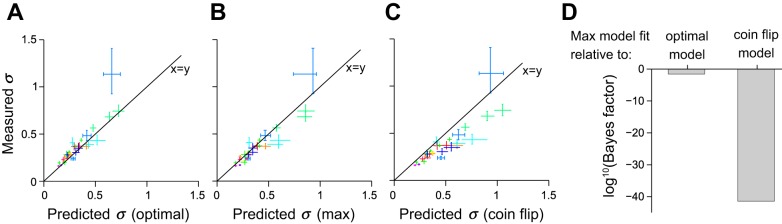
Evidence for a probabilistic decision strategy instructed by reliability. A: points relate measured sensitivity (estimated by σ; see Fig. 3A) on multisensory trials (ordinate) vs. optimal sensitivity predicted by the Bayesian model (abscissa). Each point represents a single subject on multisensory trials consisting of auditory and visual stimuli of varying reliability. Each subject contributed 3 points, 1 for each level of visual reliability. Points corresponding to the same subject are of the same color. Error bars indicate percentiles of the bootstrap distributions (1,000 samples). Points that lie on the x = y line indicate that the subject's measured performance on multisensory trials matched the optimal prediction exactly. Many subjects lie in close proximity to the x = y line. B and C: same as A except the horizontal axis shows predicted values for the max model (B) and coin flip model (C). D: Bayesian model comparison of optimal and coin flip model to max model. The max model wins, with the optimal model being a close second. The coin flip model is extremely unlikely to account for the data.

To ensure that subjects' decisions were informed by the numerosity of the stimulus and not only by its duration, we performed a probit logistic regression with both numerosity and duration as predictors. Because duration and numerosity are not perfectly correlated, this analysis allows us to isolate their relative influence on subjects' decisions. The logistic regression was performed separately for each subject, modality, and reliability level, for a total of 75 conditions.

RESULTS

We measured behavior in 11 human volunteers to determine whether subjects take into account stimulus reliability when making numerosity decisions about multisensory stimuli. Assuming that the visual and auditory estimates of numerosity are corrupted by zero mean noise with variances σ_vis² and σ_aud², the optimal strategy is to weight the two unisensory estimates in proportion to their normalized reliability (or inverse variance). In other words, the more reliable unisensory estimate should contribute more to the multisensory estimate. This strategy requires knowledge of the reliability of each unisensory estimate, which is available if the brain represents numerosity probabilistically.

The optimal model also predicts that multisensory decisions will be more precise than either of the unisensory estimates (Alais and Burr 2004; Ernst and Banks 2002; Fetsch et al. 2009, 2012; Jacobs 1999; Raposo et al. 2012; Sheppard et al. 2013; van Beers et al. 1996), as specified by Eq. 1. Numerosity judgments of a representative subject at a single reliability are shown in Fig. 3A. The psychometric function for multisensory decisions (Fig. 3A, blue curve) is steeper than that for either auditory or visual decisions (Fig. 3A, black and green curves), indicating greater precision. For this individual subject, the improvement was significant (N = 4,283 trials; σ_mult = 0.1657; σ_aud = 0.2565; σ_vis = 0.2172; P < 0.001, bootstrapping).

Fig. 3.

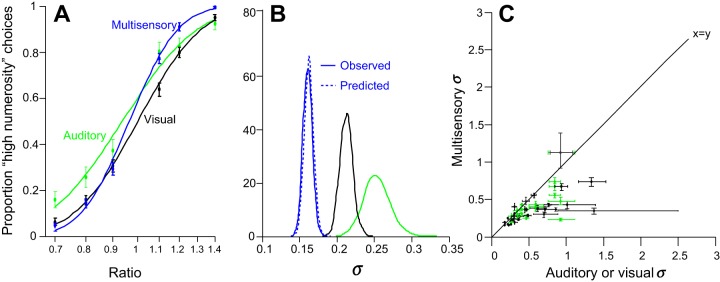
Multisensory improvement in numerosity decisions. A: psychometric functions relating the numerosity ratio of the stimulus to the proportion of times subjects reported that the numerosity was greater than the criterion. Color indicates modality. Points are data collected from a single subject (10 sessions, N = 4,283 trials); smooth lines are fits from a cumulative Gaussian function. The σ parameter from the fit is a diagnostic of subjects' sensitivity. A small value of σ indicates good performance. The steeper psychometric function for multisensory trials (blue curve) indicates more precise judgments compared with unisensory trials (black and green curves). B: a quantitative comparison of the same subject's sensitivity (estimated by σ) for each modality. Colors are the same as in A. Distributions reflect bootstrapped estimates that are computed from 1,000 resampled fits to the data. Solid lines indicate distributions of σ obtained from the performance on each condition; dashed line indicates predicted multisensory σ based on optimal combination of the single sensory data. Example subject is near optimal. C: population data. Points are data from individual subjects on a pair of conditions defined by modality and reliability. Color indicates modality: green points relate performance on unisensory auditory trials vs. multisensory trials; black points relate performance on unisensory visual trials vs. multisensory trials. Most subjects contribute 4 points to the plot, 1 for each of the 3 visual reliabilities and 1 for the single auditory reliability. Abscissa indicates performance on unisensory trials (auditory or visual) defined by σ, the parameter from the cumulative Gaussian fit that defines sensitivity (see Fig. 2). Ordinate is the same as the abscissa but for multisensory trials. Error bars are estimated by bootstrapping (1,000 samples). Points below the solid x = y line indicate subjects that were more precise for multisensory vs. unisensory trials.

Next, we tested whether the measured multisensory performance matched the predictions from the optimal model in Eq. 1 on the basis of measured unisensory performance (Fig. 3B, black and green solid lines). Importantly, this approach generates a distribution of parameters, obtained using bootstrapping, for both the measured and predicted multisensory precisions. The near match between the predicted and actual distributions shows that the multisensory improvement of the subject is close to optimal.

This improvement was consistent: for most subjects and conditions, the precision of multisensory decisions was improved relative to unisensory decisions (Fig. 3C, 21 of 30 points are below the line presenting x = y; 8 were individually significant, bootstrap, P < 0.05). We further tested multisensory improvement on a population level by evaluating min(σ_vis, σ_aud)/σ_mult across subjects and reliabilities. We found this quotient to be on average significantly smaller than 1, showing that average performance on multisensory trials was significantly better than that of unisensory trials (1-sided t-test, P = 0.015). On average, subjects were unbiased on multisensory trials (μ from the cumulative Gaussian fit was not significantly different from 0, P = 0.568). The unbiased choices on multisensory trials reflected an improvement over unisensory trials. Subjects showed idiosyncratic biases on auditory trials (although μ was not significantly different from 0, P = 0.09) and an overall weak bias for low numerosities on visual trials (μ was significantly >0, P = 0.02). The low numerosity bias on visual trials may indicate that the low signal-to-noise caused subjects to miss individual flashes.

In addition, the performance of the population was frequently close to the optimal prediction (Eq. 1). To systematically compare predicted versus optimal performance, we plotted the measured sensitivity on multisensory trials against the optimal sensitivity predicted by the Bayesian model (Fig. 4A). We found that for many subjects and reliabilities, the measured sensitivity lies in close proximity to the predicted sensitivity, supporting our hypothesis that subjects perform near-optimal multisensory integration of numerosity. The multisensory sensitivity in 22 of 30 subjects and reliabilities, when tested separately, did not differ significantly from the optimal prediction (bootstrap, P > 0.05). To ensure that subjects' decisions were informed by the numerosity of the stimulus and not only stimulus duration, we performed logistic regression. This measures the degree to which numerosity influenced decisions, taking into account that numerosity and duration are weakly correlated (see methods). We found that in 72 of 75 conditions (each a unique combination of a single subject, modality, and reliability), the effect of numerosity on choice was consistently significant and always influenced choice in the same way (choice regressor significantly >0, indicating that higher numerosity led to more “high-numerosity” choices; P < 0.05, Wald test). The effect of stimulus duration on choice, by contrast, was only inconsistently significant and had a variable influence on choice (long-duration trials led to significantly more high-numerosity choices in 42 conditions and to significantly more low-numerosity choices in 7 conditions; P < 0.05, Wald test). These results indicate that subjects were nearly always influenced by numerosity but were unable to entirely suppress duration information.

Because of the correlation between the numerosity and duration regressors, our finding of a significant numerosity effect might be sensitive to outliers in a subset of conditions. In each of the 75 conditions, we also performed a more robust nonparametric permutation test on the orthogonalized numerosity label (1,000 permutations) while keeping the original duration label (Potter 2005). We found that the numerosity coefficient is significant (P < 0.05) in the same 72 conditions as under the parametric Wald test described above. This analysis further confirms that subjects were nearly always influenced by numerosity.

Although subjects consistently estimated numerosity better on multisensory trials, their improvement deviated slightly from optimality in some cases. It is therefore possible that a suboptimal strategy, and in particular one that does not take into account the reliability of the visual and auditory cue, could account for our data. To explore this possibility, we used Bayesian model comparison to determine whether two alternatives to the optimal model could better fit the trial-by-trial choices (see methods).

The max model (Eq. 2, Fig. 4B) corresponds to a probabilistic strategy in which subjects base the decision on the more reliable modality instead of weighting the individual estimates. This strategy is suboptimal but is very close to optimal if one modality is far more reliable than the other.

By contrast, the coin flip model (Eq. 3, Fig. 4C) does not take reliability into account and would provide evidence against a probabilistic number representation. According to this strategy, the subjects randomly select the modality on which the decision is based. It predicts a performance equal to the max model for equal unisensory reliabilities but falls behind the max model for unequal unisensory reliabilities.

Figure 4D shows the performance of the max model relative to the optimal and coin flip models. For both the optimal and the coin flip models, the log of this ratio is negative, indicating that the max model is the most likely one given our data. The optimal model is a close second with a log Bayes factor of −1.6, compared with −41.5 for the coin flip model. This implies that the coin flip model is extremely unlikely to account for our data.

Finally, we restricted the model comparison to those 9 of 11 subjects for whom we varied the reliability on a trial-by-trial basis, which prevents subjects from being able to systematically ignore the less reliable modality. For this restricted pool of subjects, the max model was again the most likely, followed by the optimal model with a log Bayes factor of −7.2 and the coin flip model with a log Bayes factor of −33.

DISCUSSION

We found that human subjects can combine multiple sensory sources to refine their representation of numerosity, resulting in better performance when combining visual and auditory cues compared with using either cue alone. Moreover, subjects appear to either pick the most reliable modality on a given trial (max model) or to combine the two cues linearly with weights proportional to the reliability of each cue (optimal model). Both strategies require that human subjects encode the reliability of the numerosity estimates provided by each modality. This supports our hypothesis that subjects represent numerosity probabilistically and can exploit those representations when making decisions.

Our results are broadly consistent with previous attempts to measure multisensory number estimates (Jordan and Baker 2011; Jordan et al. 2008; Vo et al. 2014). However, our study goes far beyond existing work in that we measured responses in well-trained subjects and explicitly measured the effect of manipulating reliability, the strongest test for a probabilistic representation. We observed that reliability influences how stimuli are combined. This finding cannot be described with existing quantitative behavioral models in which the approximate number system extracts and represents a scalar estimate (see Dehaene 2007 for review). Instead, our results are consistent with neural circuits that encode numerosity probabilistically, perhaps by representing an entire distribution over numerosities, or at the very least, the mean and the variance (inverse reliability) of this distribution. Indeed, our results were best captured by models that leveraged the reliability of each cue. The results were largely incompatible with the coin flip model, which does not have a representation of reliability.

Subjects may have obtained an estimate of reliability from a number of sources. A commonly held assumption is that subjects acquire reliability estimates by inverting the generative model of the stimulus (Bishop 2006). A second possibility is that subjects estimate reliability using stimulus duration. Indeed, if the ease of detecting individual events makes duration estimates more reliable for brighter stimuli, leveraging duration to estimate reliability could be a sensible strategy. In our experiment and as reported by others (Ernst and Banks 2002; Knill and Saunders 2003), the source of the reliability estimate cannot be known precisely. Future experiments that independently vary multiple possible sources of reliability are needed to resolve this issue fully.

Although our data support the notion that humans use probabilistic representations for numerosity, we did find deviations from optimal integration. Across all subjects, the best model is the max model, according to which subjects pick the most reliable source on each trial. This strategy leads to near-optimal performance, but it is nonetheless suboptimal. This stands in contrast with other reports for optimal multisensory integration in other domains (Ernst and Banks 2002; Fetsch et al. 2012; Jacobs 1999; Raposo et al. 2012; van Beers et al. 1996). Several factors may have contributed to our finding. First, the suboptimality was only revealed by the Bayesian model comparison, which previous studies have rarely performed. If our conclusions had relied only on the analysis of behavioral thresholds, as most studies have done, it would have been tempting to conclude that our subjects were indeed optimal (Figs. 3 and 4A). This argues that future multisensory studies should include the max model as a candidate strategy. Second, there was a substantial amount of subject-to-subject variability: the performance of some subjects was better described by the max model and that of others by the optimal model. This variability in both performance and adherence to the optimal prediction is common on multisensory tasks (Rosas et al. 2005, 2007; Zalevski et al. 2007). The overall Bayesian model comparison weights each subject according to the amount of data we were able to collect from him or her. Because we were able to collect more data from some subjects than from others, the winning model depends to some degree on which strategy the subjects with more data happened to follow. Third, subjects cannot be optimal without training because they have to learn the statistics of the sensory input they are exposed to in order to be optimal. Our task is particularly challenging because it involves a comparison against an arbitrary reference (= 10). It is possible that some of our subjects did not receive sufficient training to achieve optimality. Finally, some subjects may have experienced “interference” because the auditory and visual stimuli were played asynchronously. We used stimulus rates for which a majority of subjects cannot detect audiovisual synchrony (Burr et al. 2009), but there may have been a few subjects for whom the asynchrony was apparent and caused confusion.

Our findings suggest that numerosity is represented probabilistically but leave unanswered how such probabilistic representations are encoded in the brain. Candidate areas are in the frontal and parietal cortices, both of which have been implicated as supporting numerosity estimates in humans (Castelli et al. 2006; Naccache and Dehaene 2001) and monkeys (Nieder and Miller 2004; Sawamura et al. 2002). One possibility is that neural circuits in these regions use a code known as probabilistic population code (Ma et al. 2006). Probabilistic population codes have been shown to be particularly well-suited to perform optimal multisensory integration that can be implemented by a simple linear combination of neural activities (Fetsch et al. 2012; Ma et al. 2006). Implementing multisensory integration with probabilistic population codes requires the existence of two separate unisensory populations whose activity is combined to drive a multisensory population. There is experimental evidence for all three types of populations. Recently, a study by Nieder (2012) tested trained monkeys in a multimodal comparison task and indeed was able to find groups of neurons in parietal and frontal areas that encoded either the number of auditory pulses or the number of visual items, or both. Whether the multimodal neurons add their input linearly remains to be tested, although this prediction appears to be true in other domains, such as the integration of visual and vestibular information for estimating heading (Fetsch et al. 2012; Morgan et al. 2008).

Our observation that the brain leverages probabilistic representations for numerosity decisions opens the possibility that other kinds of mathematical operations might likewise rely on probabilistic computations. For example, the approximate number system can be used not only to estimate numerosity but also to sum quantities together. Recent work (Beck et al. 2011) has shown that neural circuits with divisive normalization, a commonly found nonlinearity in neural circuits (Carandini and Heeger 2012), can implement optimal addition with probabilistic population codes. However, whether summing and increasingly complex computations rely on probabilistic inference remains an open and experimentally tractable question.

GRANTS

A. K. Churchland was supported by National Science Foundation (NSF) Grant NSF1111197 and A. Pouget by NSF1109366.

DISCLOSURES

No conflicts of interest, financial or otherwise, are declared by the authors.

AUTHOR CONTRIBUTIONS

I.K., A.P., and A.K.C. conception and design of research; I.K., A.B., and A.K.C. analyzed data; I.K., A.B., A.P., and A.K.C. interpreted results of experiments; I.K. and A.K.C. prepared figures; I.K. and A.K.C. drafted manuscript; I.K., A.P., and A.K.C. edited and revised manuscript; I.K., A.B., A.P., and A.K.C. approved final version of manuscript; A.B. performed experiments.

REFERENCES

- Alais D, Burr D. The ventriloquist effect results from near-optimal bimodal integration. Curr Biol 14: 257–262, 2004. [DOI] [PubMed] [Google Scholar]
- Bahrami B, Olsen K, Latham PE, Roepstorff A, Rees G, Frith CD. Optimally interacting minds. Science 329: 1081–1085, 2010. [DOI] [PMC free article] [PubMed] [Google Scholar]
- Beck JM, Latham PE, Pouget A. Marginalization in neural circuits with divisive normalization. J Neurosci 31: 15310–15319, 2011. [DOI] [PMC free article] [PubMed] [Google Scholar]
- Bishop CM. Pattern Recognition and Machine Learning. New York: Springer, 2006. [Google Scholar]
- Burr D, Silva O, Cicchini GM, Banks MS, Morrone MC. Temporal mechanisms of multimodal binding. Proc Biol Sci 276: 1761–1769, 2009. [DOI] [PMC free article] [PubMed] [Google Scholar]
- Carandini M, Heeger DJ. Normalization as a canonical neural computation. Nat Rev Neurosci 13: 51–62, 2012. [DOI] [PMC free article] [PubMed] [Google Scholar]
- Castelli F, Glaser DE, Butterworth B. Discrete and analogue quantity processing in the parietal lobe: a functional MRI study. Proc Natl Acad Sci USA 103: 4693–4698, 2006. [DOI] [PMC free article] [PubMed] [Google Scholar]
- Chochon F, Cohen L, Van de Moortele P, Dehaene S. Differential contributions of the left and right inferior parietal lobules to number processing. J Cogn Neurosci 11: 617–630, 1999. [DOI] [PubMed] [Google Scholar]
- Cohen MA, Grossberg S. Absolute stability of global pattern formation and parallel memory storage by competitive neural networks. IEEE Trans Syst Man Cybern 13: 815–826, 1983. [Google Scholar]
- Cordes S, Gallistel C, Gelman R, Latham P. Nonverbal arithmetic in humans: light from noise. Percept Psychophys 69: 1185–1203, 2007. [DOI] [PubMed] [Google Scholar]
- D'Errico J. Adaptive Robust Numerical Differentiation (Online). The MathWorks, Inc. http://www.mathworks.com/matlabcentral/fileexchange/13490-adaptive-robust-numerical-differentiation/content/DERIVESTsuite/hessian.m [December 18, 2013].
- Dehaene S. The neural basis of the Weber-Fechner law: a logarithmic mental number line. Trends Cogn Sci 7: 145–147, 2003. [DOI] [PubMed] [Google Scholar]
- Dehaene S. The Number Sense: How the Mind Creates Mathematics. New York: Oxford University Press, 2011. [Google Scholar]
- Dehaene S. Symbols and quantities in parietal cortex: elements of a mathematical theory of number representation and manipulation. In: Attention and Performance XXII: Sensorimotor Foundations of Higher Cognition, edited by Haggard P, Rossetti Y. Oxford: Oxford University Press, 2007, p. 527–574. [Google Scholar]
- Dehaene S, Changeux JP. Development of elementary numerical abilities: a neuronal model. J Cogn Neurosci 5: 390–407, 1993. [DOI] [PubMed] [Google Scholar]
- Deneve S, Latham PE, Pouget A. Efficient computation and cue integration with noisy population codes. Nat Neurosci 4: 826–831, 2001. [DOI] [PubMed] [Google Scholar]
- Efron B. Better bootstrap confidence intervals. J Am Stat Assoc 82: 171–185, 1987. [Google Scholar]
- Ernst MO, Banks MS. Humans integrate visual and haptic information in a statistically optimal fashion. Nature 415: 429–433, 2002. [DOI] [PubMed] [Google Scholar]
- Fetsch CR, Pouget A, DeAngelis GC, Angelaki DE. Neural correlates of reliability-based cue weighting during multisensory integration. Nat Neurosci 15: 146–154, 2012. [DOI] [PMC free article] [PubMed] [Google Scholar]
- Fetsch CR, Turner AH, DeAngelis GC, Angelaki DE. Dynamic reweighting of visual and vestibular cues during self-motion perception. J Neurosci 29: 15601–15612, 2009. [DOI] [PMC free article] [PubMed] [Google Scholar]
- Gallistel CR, Gelman R. Preverbal and verbal counting and computation. Cognition 44: 43–74, 1992. [DOI] [PubMed] [Google Scholar]
- Hopfield JJ. Neural networks and physical systems with emergent collective computational abilities. Proc Natl Acad Sci USA 79: 2554–2558, 1982. [DOI] [PMC free article] [PubMed] [Google Scholar]
- Izard V, Dehaene S. Calibrating the mental number line. Cognition 106: 1221–1247, 2008. [DOI] [PubMed] [Google Scholar]
- Jacobs RA. Optimal integration of texture and motion cues to depth. Vision Res 39: 3621–3629, 1999. [DOI] [PubMed] [Google Scholar]
- Jordan KE, Baker J. Multisensory information boosts numerical matching abilities in young children. Dev Sci 14: 205–213, 2011. [DOI] [PubMed] [Google Scholar]
- Jordan KE, Suanda SH, Brannon EM. Intersensory redundancy accelerates preverbal numerical competence. Cognition 108: 210–221, 2008. [DOI] [PMC free article] [PubMed] [Google Scholar]
- Kaufman EL, Lord MW, Reese TW, Volkmann J. The discrimination of visual number. Am J Psychol 62: 498–525, 1949. [PubMed] [Google Scholar]
- Knill DC, Saunders JA. Do humans optimally integrate stereo and texture information for judgments of surface slant? Vision Res 43: 2539–2558, 2003. [DOI] [PubMed] [Google Scholar]
- Kontsevich LL, Tyler CW. Bayesian adaptive estimation of psychometric slope and threshold. Vision Res 39: 2729–2737, 1999. [DOI] [PubMed] [Google Scholar]
- Kording KP, Beierholm U, Ma WJ, Quartz S, Tenenbaum JB, Shams L. Causal inference in multisensory perception. PLoS One 2: e943, 2007. [DOI] [PMC free article] [PubMed] [Google Scholar]
- Ma WJ, Beck JM, Latham PE, Pouget A. Bayesian inference with probabilistic population codes. Nat Neurosci 9: 1432–1438, 2006. [DOI] [PubMed] [Google Scholar]
- Morgan ML, DeAngelis GC, Angelaki DE. Multisensory integration in macaque visual cortex depends on cue reliability. Neuron 59: 662–673, 2008. [DOI] [PMC free article] [PubMed] [Google Scholar]
- Naccache L, Dehaene S. The priming method: imaging unconscious repetition priming reveals an abstract representation of number in the parietal lobes. Cereb Cortex 11: 966–974, 2001. [DOI] [PubMed] [Google Scholar]
- Nieder A. Supramodal numerosity selectivity of neurons in primate prefrontal and posterior parietal cortices. Proc Natl Acad Sci USA 109: 11860–11865, 2012. [DOI] [PMC free article] [PubMed] [Google Scholar]
- Nieder A, Dehaene S. Representation of number in the brain. Annu Rev Neurosci 32: 185–208, 2009. [DOI] [PubMed] [Google Scholar]
- Nieder A, Miller EK. A parieto-frontal network for visual numerical information in the monkey. Proc Natl Acad Sci USA 101: 7457–7462, 2004. [DOI] [PMC free article] [PubMed] [Google Scholar]
- Pelli D. The VideoToolbox software for visual psychophysics: transforming numbers into movies. Spat Vis 10: 437–442, 1997. [PubMed] [Google Scholar]
- Piazza M, Izard V, Pinel P, Le Bihan D, Dehaene S. Tuning curves for approximate numerosity in the human intraparietal sulcus. Neuron 44: 547–555, 2004. [DOI] [PubMed] [Google Scholar]
- Pica P, Lemer C, Izard V, Dehaene S. Exact and approximate arithmetic in an Amazonian indigene group. Science 306: 499–503, 2004. [DOI] [PubMed] [Google Scholar]
- Pinel P, Dehaene S, Riviere D, LeBihan D. Modulation of parietal activation by semantic distance in a number comparison task. Neuroimage 14: 1013–1026, 2001. [DOI] [PubMed] [Google Scholar]
- Potter DM. A permutation test for inference in logistic regression with small- and moderate-sized data sets. Stat Med 24: 693–708, 2005. [DOI] [PubMed] [Google Scholar]
- Pouget A, Beck JM, Ma WJ, Latham PE. Probabilistic brains: knowns and unknowns. Nat Neurosci 16: 1170–1178, 2013. [DOI] [PMC free article] [PubMed] [Google Scholar]
- Raposo D, Sheppard JP, Schrater PR, Churchland AK. Multisensory decision-making in rats and humans. J Neurosci 32: 3726–3735, 2012. [DOI] [PMC free article] [PubMed] [Google Scholar]
- Roitman JD, Brannon EM, Platt ML. Monotonic coding of numerosity in macaque lateral intraparietal area. PLoS Biol 5: e208, 2007. [DOI] [PMC free article] [PubMed] [Google Scholar]
- Rosas P, Wagemans J, Ernst MO, Wichmann FA. Texture and haptic cues in slant discrimination: reliability-based cue weighting without statistically optimal cue combination. J Opt Soc Am A Opt Image Sci Vis 22: 801–809, 2005. [DOI] [PubMed] [Google Scholar]
- Rosas P, Wichmann FA, Wagemans J. Texture and object motion in slant discrimination: failure of reliability-based weighting of cues may be evidence for strong fusion. J Vis 7: 3, 2007. [DOI] [PubMed] [Google Scholar]
- Sawamura H, Shima K, Tanji J. Numerical representation for action in the parietal cortex of the monkey. Nature 415: 918–922, 2002. [DOI] [PubMed] [Google Scholar]
- Shepard RN, Kilpatric DW, Cunningham JP. The internal representation of numbers. Cogn Psychol 7: 82–138, 1975. [Google Scholar]
- Sheppard JP, Raposo D, Churchland AK. Dynamic weighting of multisensory stimuli shapes decision-making in rats and humans. J Vis 13: 6, 2013. [DOI] [PMC free article] [PubMed] [Google Scholar]
- Skaggs WE, Knierim JJ, Kudrimoti HS, McNaughton BL. A model of the neural basis of the rat's sense of direction. Adv Neural Inf Process Syst 7: 173–180, 1995. [PubMed] [Google Scholar]
- Slutsky DA, Recanzone GH. Temporal and spatial dependency of the ventriloquism effect. Neuroreport 12: 7–10, 2001. [DOI] [PubMed] [Google Scholar]
- van Beers RJ, Sittig AC, van der Gon Denier JJ. How humans combine simultaneous proprioceptive and visual position information. Exp Brain Res 111: 253–261, 1996. [DOI] [PubMed] [Google Scholar]
- Vo VA, Li R, Kornell N, Pouget A, Cantlon JF. Young children bet on their numerical skills: metacognition in the numerical domain. Psychol Sci 25: 1712–1721, 2014. [DOI] [PMC free article] [PubMed] [Google Scholar]
- Wang X. Attractor network models. In: Encyclopedia of Neuroscience, edited by Squire R. Oxford: Academic, 2009, vol. 1, p. 667–679. [Google Scholar]
- Wichmann FA, Hill NJ. The psychometric function: I. Fitting, sampling, and goodness of fit. Percept Psychophys 63: 1293–1313, 2001. [DOI] [PubMed] [Google Scholar]
- Wills TJ, Lever C, Cacucci F, Burgess N, O'Keefe J. Attractor dynamics in the hippocampal representation of the local environment. Science 308: 873–876, 2005. [DOI] [PMC free article] [PubMed] [Google Scholar]
- Xu F. Numerosity discrimination in infants: evidence for two systems of representation. Cognition 89: B15–B25, 2003. [DOI] [PubMed] [Google Scholar]
- Xu F, Spelke ES. Large number discrimination in 6-month-old infants. Cognition 74: B1–B11, 2000. [DOI] [PubMed] [Google Scholar]
- Xu F, Spelke ES, Goddard S. Number sense in human infants. Dev Sci 8: 88–101, 2005. [DOI] [PubMed] [Google Scholar]
- Zalevski AM, Henning GB, Hill NJ. Cue combination and the effect of horizontal disparity and perspective on stereoacuity. Spat Vis 20: 107–138, 2007. [DOI] [PubMed] [Google Scholar]