Arctic sea ice trends, variability and implications for seasonal ice forecasting

Abstract

September Arctic sea ice extent over the period of satellite observations has a strong downward trend, accompanied by pronounced interannual variability with a detrended 1 year lag autocorrelation of essentially zero. We argue that through a combination of thinning and associated processes related to a warming climate (a stronger albedo feedback, a longer melt season, the lack of especially cold winters) the downward trend itself is steepening. The lack of autocorrelation manifests both the inherent large variability in summer atmospheric circulation patterns and that oceanic heat loss in winter acts as a negative (stabilizing) feedback, albeit insufficient to counter the steepening trend. These findings have implications for seasonal ice forecasting. In particular, while advances in observing sea ice thickness and assimilating thickness into coupled forecast systems have improved forecast skill, there remains an inherent limit to predictability owing to the largely chaotic nature of atmospheric variability.

1. Introduction

The modern satellite passive microwave record provides us with consistent estimates of Arctic sea ice extent since late 1978 by combining data from the Nimbus-7 scanning multi-channel microwave radiometer (1979–1987), the DMSP special sensor microwave/imager (1987–2007) and the special sensor microwave imager/sounder (2008–present) [1]. These data document downward linear trends in Arctic sea ice extent for all months, but with the largest trend for September, the end of the melt season (figure 1). Over the period 1979–2014, the September trend is −86 000 km² yr⁻¹, or −13.3% dec⁻¹ as referenced to the mean September extent for the period 1981–2010. Extent is defined as the area represented by all pixels with an ice concentration of at least 15%.

Figure 1.

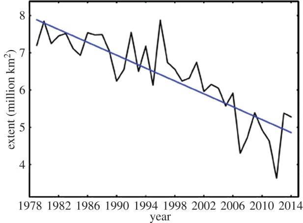
Average September sea ice extent for 1979–2014 and linear least-squares fit based on satellite passive microwave data using the NASA Team algorithm. (Adapted from NSIDC.)

It is expected that Arctic sea ice extent will continue to decline, the eventual outcome being an essentially seasonally ice-free Arctic Ocean [2]. As the Arctic loses its summer sea ice cover, the region becomes more accessible to marine transport, tourism and extraction of energy resources. While the growing economic and strategic importance of the Arctic demonstrates a need to reduce the large uncertainty as to when ice-free conditions will be realized, arguably a more urgent need is to improve seasonal forecasts of ice conditions, for even in an ice-diminished Arctic Ocean there will be large variability in conditions from year to year [3,4].

As developed in this paper, inspection of the sea ice record and analysis of other data sources reveals several notable aspects of the September trend that bear upon seasonal forecasting. First, the downward trend appears to be steepening, which is linked to the ice cover becoming younger and thinner and associated processes driven by a generally warming climate. Second, while major excursions in September ice extent from the trend line are strongly driven by variations in atmospheric circulation, large departures (more than 0.5×10⁶ km²) seldom persist more than a few years, pointing to both the general lack of persistence in atmospheric circulation patterns and a negative (stabilizing) autumn and winter feedback associated with ocean heat loss [5,6]. We follow a review of these issues with several illustrative case studies. While our analysis of sea ice variability is primarily from the viewpoint of atmospheric processes, we fully recognize that oceanic variability, such as Pacific water inflow and Atlantic water inflow, can play important roles.

2. Steepening of the trend

While the satellite sea ice record is fairly short, it is sufficiently long to conclude that the downward September trend is steepening. This is illustrated in figure 2, which compares linear trends for the first and second half of the satellite record, 1979–1996 and 1997–2014. During the first half of the time series, the rate of ice loss is −36 000 km² per year, whereas in the second half, it is four times larger, at −130 000 km² per year. This difference is statistically significant at the 99% confidence level. The smoothed curved line computed using locally weighted scatterplot smoothing [7] provides us with additional support for a significant change in the rate of ice loss. A prominent manifestation of the steeper trend during the later period is that the eight lowest September extents have all occurred within the past 8 years. Another way to illustrate the steepening trend is through computing consecutive 30 year trends, using a longer sea ice record [2] that extends back to 1953 (figure 3). In this analysis, we first compute the September trend (and two standard deviation errors) centred on 1967, based on data for the period 1953–1982, then centred on 1968, using data for the period 1954–1983, and so on, up to the trend centred on the year 1999, using data for 1985–2014. Steepening of the trend with time is clearly apparent. However, it is not until the last eight 30 year periods that the trends are significantly different from those centred on years before 1990.

Figure 2.

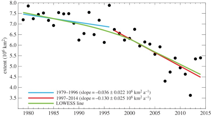
Comparison of linear trends in September sea ice extent for the period 1979–1996 and for 1997–2014. The smoothed nonlinear trend line is calculated using locally weighted scatterplot smoothing. Linear trends are calculated using least-squares regression.

Figure 3.

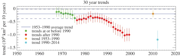
September ice extent trends over successive 30 year periods, along with 2 SD errors. The first 30 year trend period is centred on 1967, calculated from data for 1953–1982, the next is centred on 1968, calculated from data for 1954–1983, and so on. Green symbols are for trend periods that end before or on 1990. The red symbols are for trend periods that end after 1990. The blue lines show the mean and 2 SD errors for all trends ending on or before 1990. The light blue symbol shows the trend and error calculated for 1990–2014, and the orange symbol is for the trend and error computed for 1953–1990.

A key contributor to the steepening trend is the preferential loss of old ice (multi-year ice) in comparison with relatively thin first-year ice [8,9]. Information on the age of the multi-year ice is available since 1982 from Lagrangian tracking of individual ice parcels as they form, move on the Arctic Ocean surface and disappear (through melt or transport out of the Arctic) [8,10–12]. Ice age is broadly related to thickness—older ice tends to be thicker ice [11]. These data reveal a general reduction in ice age, with the loss of the oldest ice age classes (5 or more years old) being especially prominent starting in 2005. As of the year 2014, less than 5% of the Arctic Ocean consists of ice at least 5 years or older, compared with 20% in the 1980s (figure 4). Information from various sources, including submarine sonars, satellite and airborne altimeters and ice-ocean models with data assimilation, all points to thinning of the ice cover over the past several decades, consistent with the reduction in ice age [13].

Figure 4.

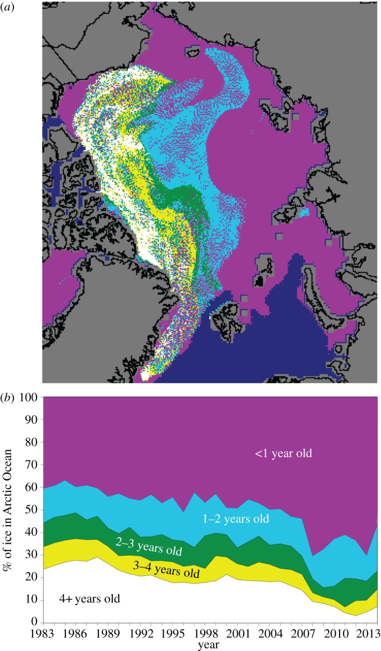
Ice age for March 2014 (a) and time series of ice age classes for March over the period 1983–2014 (b). (Adapted from NSIDC, courtesy of M. Tschudi, University of Colorado Boulder.)

However, thinning itself offers but a partial explanation—other related processes are also at work [8]. Specifically, warming in all seasons has reduced the likelihood of especially cold winters that could bring about a significant recovery in ice thickness, and has lengthened the melt season, which has in turn enhanced the ice–albedo feedback. The latter includes increased absorption of solar radiation in growing open water areas that leads to further melt.

3. Large variability but low autocorrelation

As seen in figure 1, excursions from year to year in September sea ice extent of over 1.0×10⁶ km² are not uncommon. For example, the highest September ice extent in the satellite record of 7.88×10⁶ km² that occurred in 1996 was 1.75×10⁶ km² higher than the value for the previous year, 1995 (a relative increase of 28%). Extent then dropped by more than a million km² between 1996 and 1997. The second lowest September extent in the satellite record of 4.30×10⁶ km², recorded in 2007, was 1.92×10⁶ km² below the 2006 value, a relative decrease of 45%. In turn, the record minimum extent of 3.63×10⁶ km² recorded in 2012 was followed in 2013 by a value of 5.35×10⁶ km², an increase of 1.72×10⁶ km² (nearly 50%).

Figure 5 shows the time series of September extent in terms of departures from the linear trend line. Along with highlighting that some of the departures are quite large, it shows that large departures from the trend line seldom persist for more than a couple of years. Viewed more formally, while there is a strong 1 year autocorrelation in the September extent (0.74) that results from the downward trend, when the time series is detrended, the 1 year lag autocorrelation for September is essentially zero.

Figure 5.

Departures of September sea ice extent from the linear trend line as calculated over the period 1979–2014. Particularly large departures are marked.

While consistent, long-term observations of changes in ice thickness and volume are unavailable, the pan-Arctic ice ocean modelling and assimilation system (PIOMAS) [14] provides us with estimates of volume to complement the satellite-derived extent data. Our analysis of the detrended time series from PIOMAS reveals a significant 0.58 1 year lag autocorrelation in September ice volume. That there is no 1 year lag autocorrelation in September extent while there is one in volume is not especially surprising given that volume is a more complete measure of the condition of the ice cover and the thermodynamic state of the Arctic Ocean. Extent does not necessarily scale with volume. For example, if weather conditions one summer result in anomalously low September extent, then the ocean heating through summer within the large open water areas that develop is more efficient at thinning the remaining ice. If, during the following summer, the weather patterns are more conducive for retaining ice (e.g. a thin layer of ice remains), the volume may nevertheless still decline, because the ice cover was thinner than that in the previous year.

However, the 1 year lag correlation in volume of 0.58 from PIOMAS is rather modest. We argue that both the lack of autocorrelation in extent and the very modest autocorrelation in estimated volume manifest a combination of atmospheric circulation variability and a stabilizing winter feedback.

It has long been recognized that variability in September extent, which typically has pronounced regional expressions, is strongly driven by anomalies in atmospheric circulation patterns. Such links have been variously examined in the framework of case studies (both observational and model based) for individual years [8,15–18], large-scale patterns of atmospheric variability such as the Arctic oscillation (AO) and the Arctic dipole anomaly (DA) [19–22] and from various compositing approaches [23,24]. While individual weather events at times have pronounced influences on the ice cover, what is more important in forcing variations in September extent is weather conditions integrated over time scales of at least a month, and particularly for summer.

Atmospheric circulation variability has both dynamic and thermodynamic influences. Dynamic influences involve variations in the near-surface wind field that can force sea ice convergence and divergence (e.g. offshore and onshore motion, divergence and convergence under cyclonic and anticyclonic wind stress, respectively). Thermodynamic influences involve links between circulation anomalies, horizontal temperature advection, cloud cover and snowfall, the last two influencing the surface energy balance. Dynamic and thermodynamic influences can have reinforcing impacts. For example, while anomalous southerly winds may lead to anomalous offshore ice motion, leaving areas of open water along the coast, southerly winds are also warm winds, which can accentuate summer melt.

However, summer weather conditions vary strongly from year to year [25,26]. It has been argued that, for the period 2007–2012, there was a persistent DA pattern in the June sea-level pressure (SLP) fields characterized by positive SLP anomalies centred over the Canada Basin (a strong Beaufort Sea High), and negative anomalies across northern Eurasia that enhanced the meridional flow across the Arctic [27]. The DA pattern is known to accentuate summer ice loss [18,22] (see discussion of the case study for 2006–2008). However, reflecting intra-seasonal variability, when fields for individual years are examined over this period for summer (June–August) averages, persistence is less clear, with the DA pattern best expressed for 2007 and 2011. Furthermore, summer averages for the two most recent years, 2013 and 2014, do not fit this pattern. Finally, we point out that frameworks such as the DA can be misleading as even fairly small shifts in the location of key atmospheric features, such as the Beaufort Sea High, can greatly influence patterns of sea ice motion and temperature.

The other key driver of sea ice variability, reflected in the lack of autocorrelation in the detrended September sea ice extent (and modest autocorrelation with volume), is that autumn and winter heat loss acts as a strong negative (stabilizing) feedback [5,8]. If anomalous atmospheric forcing leads to a large negative anomaly in September ice extent, there will also be large oceanic heat losses in autumn and winter from open water areas that in turn foster a large production of new ice. One manifestation of this ocean heat loss is that autumns following large negative anomalies in extent are attended by large positive anomalies in surface and lower tropospheric air temperatures. Indeed, the downward trend in September ice extent is one of the major drivers of Arctic amplification—the observed outsized rise in surface and lower tropospheric temperatures in the Arctic relative to the hemispheric average [28,29]. It follows that, unless a September with a large negative sea ice anomaly is followed by another summer with weather conditions favouring ice loss such as the DA pattern, extent will tend to climb back towards the trend line.

This stabilizing effect of ocean heat loss finds observational support in observed year-to-year changes in September sea ice extent. It is evident from figures 1 and 5 that years which have exhibited a strong negative change compared with the previous year (e.g. 2006–2007, 2011–2012) have been followed the next year by a positive change (and vice versa). Looking at the September time series as a whole, there is a modest but statistically significant negative (−0.51) 1 year lag autocorrelation in year-to-year differences in extent. These results are similar to those presented by Notz & Marotzke [6]. While this stabilizing feedback will act against the observed recent acceleration of the downward September trend in extent, apparently, it is insufficient to remove it.

It is reasonable to expect that, as the sea ice cover thins, the sea ice response to atmospheric forcing will also change. In particular, with thinner spring ice, atmospheric circulation patterns favouring summer ice loss ought to become more effective in doing so, because less energy is needed to melt out areas of ice and the ice cover is also more mobile. There is evidence that such preconditioning was a factor in the extreme summer sea ice retreat observed in 2007 [18]. However, as of yet, there is no compelling evidence that changing sensitivity to atmospheric forcing has increased September sea ice variability. As assessed over 1979–2004, the standard deviation in September extent (from the raw time series) is 0.59×10⁶ km², compared with an only slightly higher value of 0.68×10⁶ km² for the past decade (2005–2014). This may change, however, as the ice thins further in response to a warming climate [3].

4. Case studies

(a). September 1995, 1996 and 1997

This first case illustrates impacts of variability in summer atmospheric circulation during a period when the ice cover was relatively thick compared with more recent summers. As already introduced, September 1996 had the highest sea ice extent in the satellite record of 7.88×10⁶ km², which is 1.75×10⁶ km² higher than the value for the previous year, 1995. This is the largest 1 year increase in extent recorded over the satellite record and represents a departure of 1.46×10⁶ km² from the trend line (figure 5). Extent then dropped by more than 1 million km² between 1996 and 1997. Figure 6 shows fields of anomalies of SLP and 925 hPa air temperature for 1995, 1996 and 1997, averaged for summer (June, July and August) based on data from the National Centers for Environmental Prediction/National Center for Atmospheric Research (NCEP/NCAR) atmospheric reanalysis [30]. Anomalies are referenced to the period 1981–2010. We use the 925 hPa level as it provides a better indicator of lower tropospheric temperatures than does the 2 m temperature, which is strongly influenced by surface processes and parametrizations in the atmospheric model.

Figure 6.

Anomalies in sea-level pressure (a–c) and 925 hPa temperature (d–f) as referenced to 1981–2010 climatology for the summers (June–August) of 1995 (a,d), 1996 (b,e) and 1997 (c,f), based on the NCEP/NCAR reanalysis.

The dominant feature of the summer of 1995 was a region of anomalously low pressure centred over the Barents Sea. However, peak anomalies were modest (about 4 hPa). Temperature anomalies at the 925 hPa level were rather small across the Arctic Ocean; the region of positive anomalies centred over the Laptev Sea is consistent with the SLP anomaly pattern, which points to winds in the area having an anomalous southerly component. The circulation and temperature patterns for 1996 stand in stark contrast. First, negative 925 hPa temperature anomalies cover almost all of the Arctic Ocean. Second, there is a pronounced region of negative SLP anomalies centred over the northern Canada Basin.

The negative SLP anomaly and mean low for the summer of 1996 is a statistical reflection of a high cyclone frequency. As first noted by Dzerdzeevskii [31] and Reed & Kunkel [32], in a climatological sense, cyclone activity over the central Arctic Ocean peaks in summer. This pattern is associated with the influx of lows generated over the Eurasian continent as well as cyclogenesis over the Arctic Ocean itself [25]. Cyclones migrating into the central Arctic Ocean, along with those generated over the ocean itself, eventually occlude and dissipate within the cyclone maximum region. Seasonal onset of the summer cyclone maximum is linked to an eastward shift in the Urals trough, development of a separate region of high-latitude baroclinicity along the Arctic Ocean coast, and migration of the core of the 500 hPa circumpolar vortex to near the Pole. However, the strength of the summer cyclone pattern is highly variable. When well developed, such as in the summer of 1996, the 500 hPa vortex is especially strong and symmetric about the Pole. When poorly developed, the opposite pattern holds, and high pressure (a strong Beaufort Sea High) dominates the central Arctic Ocean. The strength of the cyclone pattern varies strongly from year to year [25].

As seen clearly for the summer of 1996, and as documented in a number of past studies [24], a well-developed summer cyclone pattern tends to be a cold pattern. Precipitation associated with the cyclone pattern is often in the form of snow, raising the albedo. Finally, during summer, strong cyclonic wind stress tends to be associated with sea ice divergence, spreading the existing ice over a larger area. These factors, working in combination, are consistent with the much more extensive ice cover observed for September of 1996 when compared with 1995.

Based on the ice age record introduced earlier, the fraction of first-year ice was 58% in the winter of 1995/1996, 61% in the winter of 1996/1997 and 55% in the winter on 1997/1998. Thus, the cool conditions in the summer of 1996 also worked to retain a slightly higher percentage of first-year ice that then became second-year ice at the end of the melt season. However, September ice extent for 1997 was sharply lower. The mean SLP pattern for summer 1997 is characterized by near-normal values over the Canada Basin, below-normal values over northcentral Eurasia and above-normal values over extreme northern Europe. Temperatures at the 925 hPa level were near normal to slightly below normal over most of the Arctic Ocean. While it was hence by no means a warm summer over the Arctic Ocean, conditions were certainly much milder than seen in 1996. Note in this respect that, despite the strong decline in September extent between 1996 and 1997, extent for September 1997 was still above the linear trend line (figure 5).

(b). September 2006, 2007 and 2008

This case study focuses on a succession of years that saw a pronounced drop in September extent (2006–2007) followed by modest recovery (2007–2008). Recall that September 2007 had the second lowest sea ice extent in the satellite record of (4.30×10⁶ km²), which was 1.92×10⁶ km² below the September extent recorded in 2006. September 2007 ice extent was in turn 1.16×10⁶ km² below the trend line. September extent in 2008 was considerably higher than in 2007, but still well below the trend line (figure 5).

As seen in figure 7, the SLP field for the summer of 2006 was characterized by negative anomalies over most of the Arctic Ocean, but with larger negative anomalies of up to 4 hPa centred near the Pole along 90°E longitude. Temperature anomalies at the 925 hPa level were fairly small across the Arctic Ocean. By comparison, the summer of 2007 was characterized by strong positive SLP anomalies centred over the Canada Basin (a strong Beaufort Sea High), and negative anomalies across northern Eurasia. Temperature anomalies at the 925 hPa level were positive across most of the Arctic Ocean, but with a pronounced peak over the East Siberian and Chukchi Seas.

Figure 7.

Anomalies in sea-level pressure (a–c) and 925 hPa temperature (d–f) as referenced to 1981–2010 climatology for the summers (June–August) of 2006 (a,d), 2007 (b,e) and 2008 (c,f), based on the NCEP/NCAR reanalysis.

As articulated in a number of studies of the 2007 event [18,22], southerly winds between the positive pressure anomaly centre over the Canada Basin and the negative anomalies over northeastern Eurasia promoted strong melt in the East Siberian and Chukchi Seas, as well as transport of ice away from the coasts of Siberia and Alaska towards the North Pole. The pattern of SLP anomalies on the Atlantic side of the Arctic also led to a strong surface pressure gradient across Fram Strait (between Greenland and Svalbard), enhancing wind-driven transport of sea ice out of the Arctic Ocean and into the North Atlantic.

The year 2007 serves as the exemplar of the DA pattern discussed earlier. The DA pattern has been formally defined [22] through an empirical orthogonal function (EOF) analysis of seasonal mean SLP for the region north of 70°N. The first (leading) EOF mode is the AO, which for summer has a seasonal structure very similar to that shown by Ogi et al. [33]. The DA is the second mode. In this framework, the SLP anomaly pattern shown in figure 7 is consistent with the combination of a positive summer mode of the DA and a negative mode of the summer AO. By contrast, L'Heureux et al. [34] viewed the summer 2007 circulation as an extreme positive phase of the summer Pacific North American (PNA) wavetrain. In an effort to find some common ground between different studies, Serreze & Barrett [26] showed that a strong Beaufort High, such as seen in summer 2007, tends to be a feature of the positive phase of the summer PNA, the negative phase of the summer AO, as well as the positive phases of the summer DA and Pacific Decadal Oscillation. The unifying theme is that, to varying degrees, a high-latitude 500 hPa ridge associated with the Beaufort Sea High represents a centre of action in each pattern.

It has also been argued [18,22] that the ice response to the unusual atmospheric conditions observed in the summer of 2007 was accentuated by starting out the melt season with a fairly thin spring ice cover. While the ice age record shows that spring 2007 had similar proportions of first-year versus multi-year ice (64% and 34%, respectively), as observed at the start of the 1996 melt season, the proportion of ice at least 5 years old had decreased to about 11% compared with 15% in 1996. More important is where this old ice was located. In 1996, it stretched from the Beaufort and Chukchi Seas into the East Siberian and Laptev Seas, whereas, in 2007, the Chukchi and East Siberian Seas were predominantly covered by first-year ice, allowing for large ice losses in this region during summer.

Reflecting intense ocean heat loss, and manifesting the negative feedback process outlined earlier, the following autumn saw very strong positive anomalies in surface and lower troposphere air temperature over the areas of anomalous open water. By this stabilizing feedback, we would have expected a considerably higher extent in 2008 than in 2007. The recovery, however, was modest (figures 1 and 5), apparently, at least in part, because (i) summer 2008 was also fairly warm over much of the Arctic Ocean with a circulation pattern reminiscent of the DA (figure 7), (ii) there was significant basal and lateral melt that thinned the remaining multi-year ice [35], and (iii) 77% of the spring ice cover was represented by first-year ice.

Note that September extent for the following year (2009) was close to (slightly above) the linear trend line (figure 5), which hence represents a substantial increase in extent relative to 2008. This is consistent with the observation that, in contrast to the summer of 2008, the summer average temperatures at the 925 hPa level were near the climatological (1981–2010) average along essentially all of coastal Eurasia, and were slightly below average over the eastern Beaufort Sea (not shown).

(c). September 2012 compared with 2013 and 2014

This case study contrasts summer atmospheric conditions preceding the record low September extent recorded for September 2012 (3.63×10⁶ km²) with 2013, for which extent was higher by 1.72×10⁶ km² (nearly a 50% increase), and with 2014, which ended up with a September extent slightly lower than for 2013. While extent in 2012 was 1.40×10⁶ km² below the trend line, both 2013 and 2014 ended up within 0.50×10⁶ km² of the trend line (figure 5).

The atmospheric circulation pattern for the summer of 2012 (figure 8) features negative pressure anomalies centred over the East Siberian and Chukchi Seas, with peak values of about 6 hPa, and positive anomalies centred over Greenland. The pattern bears some resemblance to what was observed for the summer of 2007 (the exemplar of the DA pattern) but with the pressure anomaly centres rotated anticlockwise and of more modest magnitude. The most salient feature of 2012 is that positive temperature anomalies at the 925 hPa level cover most of the Arctic Ocean, peaking in the Beaufort Sea where the SLP anomaly pattern points to winds with an anomalous southerly component. Phrased simply, the summer pattern favoured melt. Nevertheless, peak temperature anomalies were smaller than observed in 2007. Ice thickness at the start of the melt seasonal probably played a role. Indeed, prior to the 2012 melt season, 74% of the ice cover consisted of first-year ice and less than 3% of the remaining multi-year ice was older than 4 years, pointing to a much thinner ice cover compared with conditions at the beginning of the 1996 and 2007 melt seasons. After the record minimum in 2012, the multi-year ice fraction decreased further to 23% of the ice cover. Another factor that probably contributed to the record 2012 sea ice minimum was the development of a very strong extratropical cyclone over eastern Eurasia and its subsequent migration to over the central Arctic Ocean [36]. The strong winds associated with this system helped to break up the already thin and fragmented ice cover in the Chukchi Sea and results from a modelling study suggest that warm ocean water was mixed upwards, enhancing sea ice melt [37].

Figure 8.

Anomalies in sea-level pressure (a–c) and 925 hPa temperature (d–f) as referenced to 1981–2010 climatology for the summers (June–August) of 2012 (a,d), 2013 (b,e) and 2014 (c,f), based on the NCEP/NCAR reanalysis.

By comparison, the much higher September ice extent recorded in 2013 was preceded by a summer atmospheric circulation pattern featuring negative SLP anomalies over the Atlantic sector of the Arctic and small positive anomalies over northern Eurasia—quite unlike the DA pattern. This pressure pattern favoured ice divergence, helping to maintain a higher extent. Temperature anomalies over most of the Arctic Ocean were small or negative, limiting surface melt. Compared with 2007, the SLP anomaly pattern did not favour enhanced ice export through Fram Strait. Atmospheric conditions for the summer of 2014 were also very different from those observed in 2007. We speculate that the strong autumn and winter heat loss following the record-low extent for September 2012 was a player in the recovery in extent in 2013 to near the trend line. The observed extent for September 2014 suggests that, in the absence of a summer circulation pattern like 2007 that distinctly favours ice loss, extent will tend to stay fairly near the (steepening) linear trend line.

5. Discussion

Our analysis provides evidence that the downward trend in September sea ice extent is steepening. While part of the argument for this steepening is that thinner ice in spring is simply easier to melt out in summer, several associated processes have contributed. Warming in all seasons has reduced the likelihood of especially cold winters and has lengthened the melt season [38], which has in turn enhanced the ice–albedo feedback. The latter includes increased absorption of solar radiation in growing open water areas that leads to further melt. While there is a strong 1 year autocorrelation in the raw time series of September ice extent owing to the downward trend, there is little autocorrelation in the detrended time series and only a modest autocorrelation in volume. This reflects both the inherent large variability in summer atmospheric circulation patterns and that oceanic heat loss in winter acts as a negative (stabilizing) feedback in the sea ice system. This feedback is, nevertheless, not strong enough to counter steepening of the trend.

While our focus on atmospheric circulation forcing has been on summer, we are of course aware that atmospheric forcing during other seasons can be important. Several studies have shown that a positive AO phase during winter enhances offshore ice motion from the shores of Siberia, fostering new ice production in the region that is thinner and prone to melting out the following summer. It also favours the transport of thick ice out of the Arctic Ocean through Fram Strait. For example, during the winters of the late 1980s through the middle 1990s, the winter AO was in a generally positive phase, consistent with the emergence of strong negative anomalies in September ice extent along the shores of Siberia and a reduction in thick ice storage [19,20]. However, since that time, the AO has bounced between positive and (in several cases extreme) negative phases.

The importance of the negative feedback in autumn and winter was highlighted in a coupled climate model sensitivity study by Tietsche et al. [5] that focused on the evolution towards seasonally ice-free conditions. This study was motivated by concerns over a potential ‘tipping point’ in the sea ice system, namely that as the climate warms and the spring sea ice cover thins in response to rising greenhouse gas levels, a strong kick from natural climate variability can more easily induce a reduction in sea ice extent sufficiently large to set the albedo feedback process into high gear. As a result, the path of a general downward trend in summer ice cover would be interrupted by sudden plunges spanning a decade or more, hastening the slide to a seasonally ice-free ocean [39].

Teitsche et al. started with standard simulations driven by the IPCC A1B greenhouse gas emissions scenario for the twenty-first century. In these simulations, seasonally ice-free conditions were typically reached around the year 2070. They then performed simulations whereby every 20 years the entire sea ice cover was removed on 1 July. Instead of maintaining ice-free conditions, ice extent in September recovered to values typical of the standard runs within a couple of years, even in the later parts of the century. Why this occurs is that ocean heat loss in autumn and winter results in enough ice growing to survive the next summer's melt.

The issues discussed in our paper are highly relevant to seasonal ice forecasting. This is highlighted by Stroeve et al. [40], who examined forecasts of September sea ice extent submitted to the SEARCH Sea Ice Outlook between 2008 and 2013 (http://arcus.org/sipn/sea-ice-outlook). Contributors employ a variety of methods to forecast September sea ice extent, starting up to three months out (June), including heuristic, statistical and coupled ice–ocean or ice–ocean–atmospheric models with and without data assimilation. The median prediction of the contributions has tended to be accurate in some years but less so in others. Years when the predictions were less skilful were those for which the extent deviated from persistence. An update to the analysis (figure 9) shows that predictions for 2014 were better than those for 2013 and 2012, but not as good as for 2008, 2010 and 2011. The ensemble of all predictions from 2008 to 2014 has a root-mean-square-error (RMSE) of 0.73×10⁶ km². While this RMSE is considerably lower than that of the climatological mean (1.82×10⁶ km²), it is only slightly better than that of the linear trend (0.76×10⁶ km²). Thus, while existing studies (see [41] for a summary) suggest that ice extent should be predictable for 2 years after initialization, when these models are used to forecast the September extent, they show significant degradation of skill.

Figure 9.

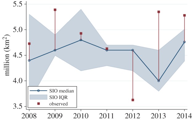
Mean and interquartile range of July SEARCH Sea Ice Outlook predictions compared with observed September mean sea ice extent from 2008 to 2014. (Courtesy of Larry Hamilton.)

The degradation of skill may, in part, be a result of inadequate initial conditions for data assimilation. Day et al. [42] suggest that improved predictability will result from better observations of sea ice thickness to initialize forecasts. This is expected given that the steepening trend in September ice extent is in part linked to a thinning ice cover. Predictive skill may increase by incorporating improved model physics. Accurate modelling of summer melt ponds provides an example [43].

However, as discussed above, atmospheric variability provides an inherent limit on sea ice predictability. For example, while 2013 started out with a large fraction of thin, first-year ice following the record minimum of 2012, comparatively benign summer weather conditions enabled a large fraction of that thin ice to survive, which was not foreseen by the forecasting community. Thus, while we expect sea ice extent to continue to decline in response to forcing from atmospheric greenhouse gases, interannual departures from this long-term trend will remain hard to predict.

Data accessibility

NCEP/NCAR Reanalysis: http://www.esrl.noaa.gov/psd/data/reanalysis/reanalysis.shtml. NSIDC Sea Ice Index: http://nsidc.org/data/seaice_index/archives.html.

Funding statement

This study was supported by NASA grant no. NNX12AB75G.

References

- 1.Fetterer F, Knowles K, Meier W, Savoie M. 2002. Sea ice index. National Snow and Ice Data Center, Boulder, CO. [Google Scholar]
- 2.Stroeve JC, Kattsov V, Barrett A, Serreze M, Pavlova T, Holland M, Meier WN. 2012. Trends in Arctic sea ice extent from CMIP5, CMIP3 and observations. Geophys. Res. Lett. 39, 19502 ( 10.1029/2012GL052676) [DOI] [Google Scholar]
- 3.Holland MM, Bailey DA, Vavrus S. 2011. Inherent sea ice predictability in the rapidly changing Arctic environment of the community climate system model, version 3. Clim. Dyn. 36, 1239–1253. ( 10.1007/s00382-010-0792-4) [DOI] [Google Scholar]
- 4.Tietsche S, Notz D, Jungclaus JH, Marotzke J. 2013. Predictability of large interannual Arctic sea-ice anomalies. Clim. Dyn. 41, 2511–2526. ( 10.1007/s00382-013-1698-8) [DOI] [Google Scholar]
- 5.Tietsche S, Notz D, Jungclaus JH, Marotzke J. 2011. Recovery mechanisms of Arctic summer sea ice. Geophys. Res. Lett. 38, 02707 ( 10.1029/2010GL045698) [DOI] [Google Scholar]
- 6.Notz D, Marotzke J. 2012. Observations reveal external driver for Arctic sea-ice retreat. Geophys. Res. Lett. 39 ( 10.1029/2012GL051094) [DOI] [Google Scholar]
- 7.Cleveland WS, Devlin SJ. 1988. Locally-weighted regression: an approach to regression analysis by local fitting. J. Am. Stat. Assoc. 83, 596–610. ( 10.2307/2289282) [DOI] [Google Scholar]
- 8.Stroeve JC, Serreze MC, Kay JE, Holland MM, Meier WN, Barrett AP. 2012. The Arctic's rapidly shrinking sea ice cover: a research synthesis. Clim. Change 110, 1005–1027. ( 10.1007/s10584-011-0101-1) [DOI] [Google Scholar]
- 9.Comiso JC, Parkinson CL, Gersten R, Stock L. 2008. Accelerated decline in the Arctic sea ice cover. Geophys. Res. Lett. 35, 01703 ( 10.1029/2007GL031972) [DOI] [Google Scholar]
- 10.Fowler C, Emery WJ, Maslanik J. 2004. Satellite-derived evolution of Arctic sea ice age: October 1978 to March 2003. IEEE Geosci. Remote Sens. Soc. Lett. 1, 71–74. ( 10.1109/LGRS.2004.824741) [DOI] [Google Scholar]
- 11.Maslanik JA, Fowler C, Stroeve J, Drobot S, Zwally J, Yi D, Emery W. 2007. A younger, thinner Arctic ice cover: increased potential for rapid extensive sea ice loss. Geophys. Res. Lett. 34, 24501 ( 10.1029/2007/GL032043) [DOI] [Google Scholar]
- 12.Maslanik J, Stroeve J, Fowler C, Emery W. 2011. Distribution and trends in Arctic sea ice age through spring 2011. Geophys. Res. Lett. 38, 13502 ( 10.1029/2011GL047735) [DOI] [Google Scholar]
- 13.Stroeve JC, Barrett A, Serreze M, Schweiger A. 2014. Using records from submarine, aircraft and satellite to evaluate climate model simulations of Arctic sea ice thickness. Cryosphere 8, 1–13. ( 10.5194/tc-8-1-2014) [DOI] [Google Scholar]
- 14.Zhang JL, Rothrock DA. 2003. Modeling global sea ice with a thickness and enthalpy distribution model in generalized curvilinear coordinates. Mon. Weather Rev. 131, 845–861. ( 10.1175/1520-0493(2003)131<0845:MGSIWA>2.0.CO;2) [DOI] [Google Scholar]
- 15.Lynch AH, Maslanik JA, Wu W. 2001. Mechanisms in the development of anomalous sea ice extent in the western Arctic: a case study. J. Geophys. Res. 106, 28097–28105. ( 10.1029/2001JD000664) [DOI] [Google Scholar]
- 16.Serreze MC, Maslanik JA, Key JR, Kokaly RF, Robinson DA. 1995. Diagnosis of the record minimum in Arctic sea ice area during 1990 and associated snow cover extremes. Geophys. Res. Lett. 22, 2183–2186. ( 10.1029/95GL02068) [DOI] [Google Scholar]
- 17.Maslanik JA, Serreze MC, Agnew T. 1999. On the record reduction in 1998 western Arctic sea-ice cover. Geophys. Res. Lett. 26, 1905–1908. ( 10.1029/1999GL900426) [DOI] [Google Scholar]
- 18.Stroeve J, Serreze M, Drobot S, Gearheard S, Holland M, Maslanik J, Meier W, Scambos T. 2008. Arctic sea ice extent plummets in 2007. EOS, Trans. Am. Geophys. Union 89, 13–14. ( 10.1029/2008EO020001) [DOI] [Google Scholar]
- 19.Rigor IG, Wallace JM, Colony RL. 2002. Response of sea ice to the Arctic oscillation. J. Clim. 15, 2648–2663. ( 10.1175/1520-0442(2002)015<2648:ROSITT>2.0.CO;2) [DOI] [Google Scholar]
- 20.Rigor IG, Wallace JM. 2004. Variations in the age of Arctic sea-ice and summer sea-ice extent. Geophys. Res. Lett. 31, 09401 ( 10.1029/2004GL019492) [DOI] [Google Scholar]
- 21.Ogi M, Wallace JM. 2007. Summer minimum Arctic sea ice extent and the associated summer atmospheric circulation. Geophys. Res. Lett. 34, 12705 ( 10.1029/2007GL029897) [DOI] [Google Scholar]
- 22.Wang J, Zhang J, Watanabe E, Ikeda M, Mizobata K, Walsh JE, Bai X, Wu B. 2009. Is the dipole anomaly a major driver to record lows in Arctic summer sea ice extent? Geophys. Res. Lett. 36, 05706 ( 10.1029/2008GL036706) [DOI] [Google Scholar]
- 23.Rogers JC. 1978. Meteorological factors affecting interannual variability of summertime ice extent in the Beaufort Sea. Mon. Weather Rev. 106, 890–897. ( 10.1175/1520-0493(1978)106<0890:MFAIVO>2.0.CO;2) [DOI] [Google Scholar]
- 24.Screen JA, Simmonds I, Keay K. 2011. Dramatic interannual changes of perennial Arctic sea ice linked to abnormal summer storm activity. J. Geophys. Res. 116, 1984–2012. ( 10.1029/2011JD015847) [DOI] [Google Scholar]
- 25.Serreze MC, Barrett AP. 2008. The summer cyclone maximum over the central Arctic Ocean. J. Clim. 21, 1048–1065. ( 10.1175/2007JCLI1810.1) [DOI] [Google Scholar]
- 26.Serreze MC, Barrett AP. 2011. Characteristics of the Beaufort Sea High. J. Clim. 24, 159–182. ( 10.1175/2010JCL3636.1) [DOI] [Google Scholar]
- 27.Overland JE, Francis JA, Hanna E, Wang M. 2012. The recent shift in early summer atmospheric circulation. Geophys. Res. Lett. 39, 19804 ( 10.1029/2012GL053268) [DOI] [Google Scholar]
- 28.Serreze MC, Barrett AP, Stroeve JC, Kindig DM, Holland M. 2009. The emergence of surface-based Arctic amplification. Cryosphere 3, 9–11. ( 10.5194/tc-3-11-2009) [DOI] [Google Scholar]
- 29.Screen JA, Simmonds I. 2010. The central role of diminishing sea ice in recent Arctic temperature amplification. Nature 464, 1334–1337. ( 10.1038/nature09051) [DOI] [PubMed] [Google Scholar]
- 30.Kalnay E, et al. 1996. The NCEP/NCAR 40-year re-analysis project. Bull. Am. Meteorol. Soc. 77, 437–471. ( 10.1175/1520-0477(1996)077<0437:TNYRP>2.0.CO;2) [DOI] [Google Scholar]
- 31.Dzerdzeevskii BL. 1945. Tsirkulatsionnye skhemy v troposfere Tsentralnoi Arctike.Moscow, Russia: Izdat; Akad. Nauk SSSR. [In Russian.] (Transl. Circulation schemes for the Central Arctic troposphere. Science Report no. 3, Contract AF 19 (122)-128. Los Angeles, CA: Meteorology Department, University of California, Los Angeles.) [Google Scholar]
- 32.Reed RJ, Kunkel BA. 1960. The Arctic circulation in summer. J. Meteorol. 17, 489–506. ( 10.1175/1520-0469(1960)017<0489:TACIS>2.0.CO;2) [DOI] [Google Scholar]
- 33.Ogi M, Yamazaki K, Tachibana Y. 2004. The summertime annular mode in the Northern Hemisphere and its linkage to the winter mode. J. Geophys. Res. 109, 20114 ( 10.1029/2004JD004514) [DOI] [Google Scholar]
- 34.L'Heureux ML, Kumar A, Bell GD, Halpert MS, Higgins RW. 2008. Role of the Pacific-North American (PNA) pattern in the 2007 Arctic sea ice decline. Geophys. Res. Lett. 35, 20701 ( 10.1029/2008GL035205) [DOI] [Google Scholar]
- 35.Perovich DK, Richter-Menge JA, Jones KF, Light B. 2008. Sunlight, water and ice: extreme Arctic sea ice melt during the summer of 2007. Geophys. Res. Lett. 35, 11501 ( 10.1029/2008GL034007) [DOI] [Google Scholar]
- 36.Simmonds I, Rudeva I. 2012. The great Arctic cyclone of August 2012. Geophys. Res. Lett. 39, 23709 ( 10.1029/2012GL054259) [DOI] [Google Scholar]
- 37.Zhang J, Lindsay R, Schweiger A, Steele M. 2013. The impact of an intense summer cyclone on 2012 Arctic sea ice retreat. Geophys. Res. Lett. 40, 720–726. ( 10.1002/grl.50190) [DOI] [Google Scholar]
- 38.Stroeve JC, Markus T, Boisvert L, Miller J, Barrett A. 2014. Changes in Arctic melt season and implications for sea ice loss. Geophys. Res. Lett. 41, 1216–1225. ( 10.1002/2013GL058951) [DOI] [Google Scholar]
- 39.Holland MM, Bitz CM, Tremblay B. 2006. Future abrupt reductions in the summer Arctic sea ice. Geophys. Res. Lett. 33, 23503 ( 10.1029/2006GL028024) [DOI] [Google Scholar]
- 40.Stroeve JC, Hamilton L, Bitz C, Blanchard-Wigglesworth E. 2014. Predicting September sea ice: ensemble skill of the SEARCH sea ice outlook 2008–2013. Geophys. Res. Lett. 41, 2411–2418. ( 10.1002/2014GL059388) [DOI] [Google Scholar]
- 41.Guemas V, et al. In press A review on Arctic sea-ice predictability and prediction on seasonal to decadal time-scales. Q. J. R. Meteorol. Soc. ( 10.1002/qj.2401) [DOI] [Google Scholar]
- 42.Day J, Hawkins E, Tietsche S. 2014. Will Arctic sea ice thickness initialization improve seasonal-to-interannual forecast skill? Geophys. Res. Lett. 41, 7566–7575. ( 10.1002/grl.v41.21) [DOI] [Google Scholar]
- 43.Schröder D, Feltham DL, Flocco D, Tsamados M. 2014. September Arctic sea-ice minimum predicted by spring melt-pond fraction. Nat. Clim. Change 4, 353–357. ( 10.1038/NCLIMATE2203) [DOI] [Google Scholar]
Associated Data
This section collects any data citations, data availability statements, or supplementary materials included in this article.
Data Availability Statement