

Abstract
Dielectric spectroscopy has proved to be a good tool for analyzing the passive electrical properties of biological tissues as well as those of inhomogeneous materials. This technique promises to be a valid alternative to the classical ones based on metabolites to monitor the growth and cell volume fraction of cell cultures in a simple and minimally invasive way. In order to obtain an accurate estimation of the cell volume fraction as a function of the permittivity of the suspension, a simple in silico procedure is proposed. The procedure is designed to perform homogenization from the micro-scale to the macro-scale using simple analytical models and simulation setups hypothesizing the properties of diluted suspension (cell volume fraction less than 0.2). Results obtained show the possibility to overcome some trouble involving the analytical treatment of the cellular shape by considering a sphere with the same permittivity in the quantitative analysis of the cell volume fraction. The entire study is based on computer simulations performed in order to verify the correctness of the procedure. Obtained data are used in a cell volume fraction estimation scenario to show the effectiveness of the procedure.
Keywords: Dielectric spectroscopy, Cell volume fraction, Effective permittivity, Computer simulations
Introduction
In this work, we show a procedure that enables to predict the feasibility of the application of dielectric spectroscopy for the estimation of the cell volume fraction (CVF) of a cellular culture in order to increase the accuracy in many scenarios such as medical diagnostic procedures, food industries (e.g., beer yeast monitoring), pharmacological industry, detection of microbial water pollution, and agriculture.
The dielectric properties of biological tissues [1–3], as well as those of inhomogeneous materials in general [4], are strictly related to the shape, dimensions, and cell volume fraction (CVF) occupied by the particulate (cells) and the working frequency.
Focusing on the characterization of biological tissues, Fricke was one of the first researchers interested in giving an analytical model of the dielectric behavior of cellular suspensions [5, 6]. Over the years, this model was improved, increasing the accuracy in frequency-dependent estimations [7, 8] for simple forms such as spheres or ellipsoids. Recent advances are focused on the definition of the dielectric behavior of suspensions with more complex forms [9] in the presence of many distinct relaxation phenomena [10] and generally in the development of methods both analytical and numerical [11, 12].
Taking advantage of the β-dispersion phenomenon [13–15], it is possible to estimate the cellular CVF using dielectric spectroscopy as suggested in [16] and followed by [17–20], especially in the monoculture cases.
The theoretical study of the phenomenon in the presence of non-canonical geometries is often difficult to manage in an analytical way and the simplifications adopted in the above-mentioned works are such that their approaches do not produce accurate results. The only reasonable alternative to the study of the dielectric behavior of a cell culture is direct measurement [21–26] or the use of computer simulations.
The simplest cellular model, setting the inner structures as organelles and cell nucleus apart, is a sphere covered by a shell with a thickness of one thousandth of the sphere radius. This kind of structure, especially in 3D space, requires a far greater amount of working memory in contrast to the case of simple spheres. This is due to the large amount of grid points, or meshes, needed for the correct discretization of the shell itself and of the space around it, in order to ensure the correctness of the solution provided by the numerical solvers. Therefore, simulating the dielectric behavior even of just a few cells between two plane parallel plates may require an unavailable amount of working memory; surely a computer simulation that involves simultaneously the measuring probe and its neighborhood with manifold millions of cells may be prohibitive.
To overcome these kinds of issues, a validation procedure for dielectric behavior models is proposed and used in the case of measurement performed by a simple open-ended coaxial cable probe [27].
Methods
The dielectric spectrum of an inhomogeneous material depends on both the electromagnetic characteristics of the phases of which it is composed and by their geometry and spatial arrangement. Depending on the frequency range under consideration, one can observe the various phenomena of dielectric relaxation caused by the interaction between the electric field and the material.
In this paper, we will focus on the phenomenon of β-dispersion that strongly depends on the geometry of the non-homogeneities of the material. Having described the model of β-dispersion, we will illustrate and motivate the procedure to follow in order to obtain the estimation of the CVF starting from the dielectric spectrum of the cell culture, and finally present the results obtained from the simulation of a measurement of the dielectric spectrum.
Estimation of the effective permittivity
The β-dispersion is the typical dielectric relaxation due to the interface polarization in biological tissues in low radio-frequency range (1 kHz–100 MHz depending on the cell dimension). It is characterized by high values of the real part of the permittivity at pre-relaxation frequencies, due to the capacitance effect of the cellular membrane.
We define: ε as the relative permittivity of the medium; σ as the specific conductivity (S/m); ω as the angular frequency (rad/s) and ε0 as the vacuum permittivity 8.854 × 10⁻¹² F/m. The complex permittivity is expressible as .
Given a diluted suspension with volumetric fraction ϕ of spherical cells of radius r and membrane thickness d, immersed in a homogeneous conductive medium, the effective complex permittivity can be modeled by the Wagner mixture equation [28]:
| 1 |
where is the complex permittivity of the external medium and is the effective complex permittivity of the shell-covered sphere provided by [29]:
| 2 |
where and are respectively the complex permittivities of the shell and the cellular core.
The equations (1–2) are obtained analytically and are widely accepted, and we will use these as a reference. Similar equations are available for other geometries such as ellipsoids or cylinders [5, 6]. If the size of every cell is the same, it is simple to verify that the relaxation phenomenon is characterized by a single time constant Debye trend as described in [30]:
| 3 |
where is the suspension effective complex permittivity at high frequencies (at least a value ten times greater than the relaxation frequency value); △ε quantifies the magnitude of the dielectric jump pre- and post-relaxation and τ is the time constant of the relaxation, strongly dependent on the cell size. In this work we make use of the values in Table 1.
Table 1.
Values of electromagnetic and geometrical parameters used in this work
| Physical quantity | Value |
|---|---|
| Specific conductivity of the medium | σ a = 0.1 S/m |
| Relative permittivity of the medium | ε a = 81 |
| Specific conductivity of the membrane | σ m = 10−6 S/m |
| Relative permittivity of the membrane | ε m = 5 |
| Specific conductivity of the cell core | σ i = 0.1 S/m |
| Relative permittivity of the cell core | ε i = 81 |
| Cell radius | r = 5μm |
| Membrane thickness | d = 5 nm |
Due to the range of frequencies and the dimension of the computer simulation volume (less than a millimeter), working under the stationary-field hypothesis is possible. The effective permittivity can be obtained simply from the estimation of the global conductance G of an ideal parallel plate capacitor where the space between the plates is filled with the cellular suspension using the following equation:
| 4 |
Description of the CVF estimation procedure
It is possible to estimate the CVF of a culture using the procedure described below. It is composed of the following steps. The first step consists of replacing the original cell with a Solid sphere with the proper effective complex permittivity and the same volume. This provides a simplification in the geometry of the problem, avoiding the problem of considering the shell among the objects in the computer simulation domain.
The effective permittivity is given by the following equation obtained by the rearrangement of terms in (1):
| 5 |
The second step consists of the homogenization of the whole suspension using (1); we replace the original cells with the spheres with effective permittivity provided by the previous step and obtain the effective permittivity of the whole culture making the computer simulation of the CVF estimation setup possible.
As a third step, the effective permittivity is used for the computer simulation of a real measurement setup, in order to verify the adequacy of the measurement probe and to test the calibration procedures. In this work, the measurement of the permittivity is performed simulating an open-ended coaxial probe.
The complex permittivity estimation of the medium is performed through the measurement of the load conductance seen from the open end of the probe. Then (4) is used for the estimation of . The final step consists of the estimation of the CVF from the data acquired in the third step.
Rearranging the terms of (1), since the shape uniformity of the suspended cells is granted by the execution of the first step of the procedure, it is possible to obtain an explicit relation for the CVF, as described by the following:
| 6 |
where is the estimated value of the CVF.
Then, an estimation of the CVF from knowable physical quantities can be obtained.
Implementation of the cellular volume fraction estimation procedure
All computer simulations have been carried out using the AC/DC module of COMSOL Multiphysics using the BiGCStab [31] numerical solver. The analytical model and comparison with the simulation results are implemented in MATLAB. All software was run on a workstation with Intel Core i7 950 CPU, 24 GB RAM and Windows 7 professional OS.
The adoption of the shell-covered sphere as a reference shape is dictated by the simplicity of the analytical form of its dielectric behavior model, necessary for a first validation of the procedure, especially to test the performance of the adopted numerical solver.
The first step of the procedure considers a single shell-covered sphere placed in the middle of an ideal cylindrical capacitor. Values of core, membrane, and external-medium relative permittivity and specific conductivity, cellular radius, and shell thickness, are taken from Table 1.
A cylinder with height of 30 μm and a base radius of 15 μm is created and a single shell-covered sphere is placed in its middle. In order to obtain an ideal capacitor, null current flux boundary condition is imposed on the lateral surface while a potential difference of 1V is imposed between the flat surfaces.
In order to check the validity of the substitution procedure exposed in the previous section, the homogenization of prolate and oblate ellipsoids is executed. For simplicity, ellipsoids (both oblate and prolate) are referred to by the Cartesian reference axes. Values of complex permittivity of external medium, shell, and core of the ellipsoids are reported in Table 1. The major semi-axis of the prolate ellipsoid (with semi-axes of length 7.5 μm, 1.25 μm, 1.25 μm) is such to be aligned to the electric field as the minor semi-axis of the oblate ellipsoids (with semi-axes of length 2.22 μm, 7.5 μm, 7.5 μm). Prolate and oblate ellipsoids have the same volume.
As a result, is obtained.
The second step is performed by the computer simulations of different cell cultures with the CVF in the range [0.01–0.15]. In these simulations, we impose the value of obtained from the previous step and assigned at the effective sphere.
The assumptions, shape of the simulation domain, and the boundary condition are the same as described above; the only difference is the presence of more objects in the computer simulation domain and the size of the domain that is doubled. The number of those spheres is such to obtain the desired value of the volume fraction while the geometrical dimensions of the domain remain the same.
Thanks to the simplification of the cell geometry, saving a substantial amount of computation time and memory employment is possible. As part of the procedure, the computer simulation of the probe calibration is performed. The calibration of the coaxial probe follows the classical method using substances with known permittivity and known potential difference between the internal and external conductors (in our case, 1V). The domain of computer simulation is a cylinder 10 cm in height with a base radius of 3 cm, partially filled with air (σair = 0,εair = 1) and partially with water (εw = 81). The probe is 8 cm long with an external radius of 2.2 mm. It is filled with glass and partially embedded in the medium. The null current flux boundary condition is imposed on the lateral and the bottom surfaces, while the mass condition is imposed on the external conductor as shown in Fig. 1.
Fig. 1.
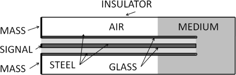
Geometry used for the simulation of the calibration and CVF estimation
As a result of this step, the shape parameter d of the probe is estimated. The final step is CVF estimation, which is performed using directly (6) or alternatively a brute-force search in order to confirm the validity of the estimation. The simulation domain is the same used for the calibration.
The brute-force method consists of solving (1) obtaining an as a function of estimated values of and varying ϕ in the interval [0, 1]; in other words, the minimum and maximum reachable by ϕ, with a step of 0.001; then the value of ϕ that assures the best accordance between computed and measured data is chosen as the CVF value. The passage from actual shape to Solid sphere for the suspended objects allows the use of (6) for its estimation.
Results
In Fig. 2, the real part of the effective permittivity obtained from (2) is compared to that obtained from (5). In the case of the spherical cell, the magnitude of the relative estimation error (see Fig. 3b) is less than 6 × 10⁻³ and decreases as the frequency increases with a similar trend as the permittivity.
Fig. 2.

Real part of equivalent permittivity of a shell-covered sphere estimated by (2) and (5) with the data obtained from the simulation
Fig. 3.

a Comparison between the equivalent permittivity obtained with (5) with the data obtained from the simulator for prolate and oblate ellipsoid (circle-marked and star-marked lines) permittivity and the reference sphere (cross-marked line). b Relative error on the computed equivalent permittivity due to the adoption of the spherical model for ellipsoids
As highlighted in (2), the effective permittivity of the sphere is independent of the actual volume fraction; then, for its estimation, carrying out a single computer simulation with a given value of ϕ (in our case ϕ = 0.0247) across the frequency range of interest is sufficient.
The substitution of the shell-covered sphere with the effective sphere improves the simulation performance both in terms of resolution time and RAM usage. The computation of the shell-covered sphere dielectric spectrum runs in 3,447 s with the use of 6.65 GB of RAM, while the effective sphere case runs in 335 s with the use of 1.68 GB of RAM.
In Fig. 3a, the behavior of the real part of the permittivity , obtained by (5) with the data provided from the simulation of prolate and oblate ellipsoids, is presented together with that of a shell-covered sphere with the same shell-radius ratio and volume obtained from (2). The CVF value of ϕ = 0.0247 is chosen in order to show the influence of the actual cellular shape on the effective permittivity values.
The discrepancy between the values of of the effective sphere reported in Figs. 2 and 3 is due to the need to double the shell thickness for the ellipsoids in order to satisfy the simulator requirement (minimum accepted value: 8 nm).
These data match the values of ε∗ provided by (1), as shown by the magnitude of the relative error reported in Fig. 3b. Then it is possible to substitute shell-covered ellipsoids with solid spheres in a totally transparent manner. Then, once is obtained and shows a Debye trend, the remaining steps of the procedure can be performed considering a suspension of solid spheres with estimated as described in the previous sections; in fact, as shown in Fig. 3b, the substitution error on the measured permittivity is under 1 × 10⁻⁶.
The values of the permittivity obtained from the execution of the first two steps of the proposed procedure are compared to those obtained with (1) and (2) and presented in Fig. 4a. The relative estimation error versus frequency is shown in Fig. 4b.
Fig. 4.

a Estimated (continuous lines) and theoretical (dotted lines) values of the real part of the complex permittivity. b Magnitude of the relative estimation error versus the frequency. Tests were performed at different volume fraction values
As shown in Fig. 4b, the error magnitude is mostly less than 5%, except for ϕ = 0.15, and generally decreases for low-volume fraction values and for higher frequency values.
The particular behavior of the relative error on the permittivity estimated in the first and second steps suggests that it is due mainly to the discrepancy between actual and desired volume fraction derived from the meshed approximate geometry. In fact, it shows a larger error at low frequencies, where the influence of the geometry on the permittivity is greater, and decreases as frequency increases until it vanishes at high frequencies, where the influence of the geometry of the suspended medium is negligible. In the case of the second step, in particular, the non-uniformity of the relative error trend along frequencies and volume fraction (note that the error is greater for ϕ = 0.03 than for ϕ = 0.09) suggests the limited correctness of the numerical solution provided by the solver used. Nevertheless, the accordance with expected values is satisfactory for our purpose.
In order to verify the accuracy of the probe calibration procedure through the permittivity range of interest, the values of permittivity obtained from (1,2) for different values of CVF are compared to the estimated values obtained from the coaxial-probe computer simulations. The magnitude of the relative error is shown in Fig. 5.
Fig. 5.

Magnitude of the relative estimation error versus frequency. Tests are performed at different volume-fraction values
The relative error is less than 2.5 × 10⁻³ for all the volume fractions considered and it does not depend significantly on the frequency. Therefore the procedure provides an accurate shape parameter d and does not introduce distortions in the measured spectrum. Thanks to the possibility to calibrate the measurement probe, the low error introduced by the previous steps allows a really good estimation of the CVF as shown in Fig. 6.
Fig. 6.

a CVF estimation values obtained from a computer simulation performed at 100 kHz with equivalent permittivity values of the suspension as presented in Fig. 2; b estimation error
When the analytical model is chosen, the relative error is always less than 3%, while in the case of the brute-force method, the error reaches 10% and in general it is greater along the permittivity range. Both methods used for the computation show good accordance with the expected values, though a better accuracy seems to be achieved by the use of (6) instead of the brute-force method.
Discussion
In this work for the first time a systematic procedure for the validation of CVF estimation via dielectric spectroscopy is presented, beginning from the definition of the cell's geometry and properties by way of the definition of the measurement probe and ending with the CVF estimation.
It can be used to define the reference dielectric behavior of a particular cell culture as well as the dielectric behavior that is possible to be expected varying some of the parameters defining the cell culture.
The working hypothesis of the dilute cell suspension and the cell geometry are dictated primarily by the necessity to evaluate the performances of the procedure using a simple, well known, and widely accepted theoretical framework.
It is possible to extend the procedure for higher-volume fractions including in the first step the study of cellular aggregate. The definition of geometries other than those presented here does not constitute a problem, since the first step transforms it in the equivalent sphere and then it remains transparent for the following steps.
The hierarchical structure of the procedure allows the working pipeline to be modified in order to adapt it to the actual case. For example, the inclusion of cell organelles in the model is possible, and a new step is carried out before the first for the homogenization of this structure.
The simulation of a cellular culture composed by different cell types is possible; the first step can be performed for every cell type in order to associate them with the proper equivalent sphere and then one can perform the homogenization of the whole culture considering the corresponding CVF of every cell type.
The introduction of a particular measurement probe in the procedure allows testing its accuracy and sensitivity in order to enable an evaluation of its adequacy. Once the calibration of the probe is done, i.e., the shape parameter d is determined, verifying the capability of the system to correctly measure the permittivity of the cell culture and then its CVF is possible.
Despite the potentialities, the capability of the proposed procedure to correctly describe a cell culture is limited by the knowledge about the cell culture itself. In particular, it is fundamental to describe the cell geometry accurately. The properties of the suspension medium are easily measurable by direct measurement; the properties of the membrane and of the core requires that such materials are isolated for the measurement.
For higher CVF values, its estimation obtained from (6) could be not accurate. Then, using the proposed procedure for the creation of a lookup table that covers the range of CVF not supported by the model is possible.
Conclusions
The in silico validation procedure for CVF estimation techniques based on dielectric spectroscopy seems to be a good tool to overcoming the actual technical limitations of dielectric spectroscopy used in CVF estimation. This is possible thanks to the accuracy demonstrated by the procedure in the description of the phenomenon, as reported in the discussion, taking full advantage of this particular measurement technique.
Despite the actual limitations, the results presented here encourage us to further develop the theory behind the dielectric behavior of cell culture in order to avoid the actual limitations of the proposed procedure.
Future works shall be centered on suspensions with cells with anisotropic dielectric behavior or in general with a certain variability of dimensions or dielectric properties of the core; moreover, it is of interest to try to estimate the electric properties of the core from the dielectric spectroscopy of the whole culture.
Acknowledgments
This work is part of the research project: Assessment techniques of three-dimensional (3D) cell growth and morphology in microgravity using electromagnetic diffraction, realized through the Italian Space Agency (ASI) co-financing.
References
- 1.Gabriel C, Gabriel S, Corthout E. The dielectric properties of biological tissues: I. Literature survey. Phys. Med. Biol. 1996;41:2231–2249. doi: 10.1088/0031-9155/41/11/001. [DOI] [PubMed] [Google Scholar]
- 2.Gabriel S, Lau RW, Gabriel C. The dielectric properties of biological tissues: II. Measurements in the frequency range 10 Hz to 20 GHz. Phys. Med. Biol. 1996;41:2251–2269. doi: 10.1088/0031-9155/41/11/002. [DOI] [PubMed] [Google Scholar]
- 3.Gabriel S, Lau RW, Gabriel C. The dielectric properties of biological tissues: III. Parametric models for the dielectric spectrum of tissues. Phys. Med. Biol. 1996;41:2271–2293. doi: 10.1088/0031-9155/41/11/003. [DOI] [PubMed] [Google Scholar]
- 4.Sihvola, A.: Electromagnetic mixing formulas and applications. The Institute of Electrical Engineers (1996)
- 5.Fricke H. The electric permittivity of a dilute suspension of membrane-covered ellipsoids. J. App. Phys. 1953;24:644–645. doi: 10.1063/1.1721343. [DOI] [Google Scholar]
- 6.Fricke H. The complex conductivity of a suspension of stratified particles of spherical or cylindrical form. J. Phys. Chem. 1955;59:168–170. doi: 10.1021/j150524a018. [DOI] [Google Scholar]
- 7.Schwan HP, Lawrence SH, Tobias CA. Electrical properties of tissue and cell suspensions. Adv. Med. Biol. Phys. 1957;5:147–152. doi: 10.1016/b978-1-4832-3111-2.50008-0. [DOI] [PubMed] [Google Scholar]
- 8.Schwan HP, Bothwell TP. Electrical properties of the plasma membrane of erythrocytes at low frequencies. Nature. 1956;178:265–266. doi: 10.1038/178265b0. [DOI] [PubMed] [Google Scholar]
- 9.Di Biasio A, Cametti C. Effect of shape on the dielectric properties of biological cell suspensions. Bioelectrochemistry. 2007;71:149–156. doi: 10.1016/j.bioelechem.2007.03.002. [DOI] [PubMed] [Google Scholar]
- 10.Di Biasio A, Cametti C. Dielectric properties of aqueous zwitterionic liposome suspensions. Bioelectrochemistry. 2007;70:328–334. doi: 10.1016/j.bioelechem.2006.04.004. [DOI] [PubMed] [Google Scholar]
- 11.Asami K. Dielectric dispersion in biological cells of complex geometry simulated by the three-dimensional finite difference method. J. Phys. D.: Appl. Phys. 2006;39:492–499. doi: 10.1088/0022-3727/39/3/012. [DOI] [Google Scholar]
- 12.Ramos A. Improved numerical approach for electrical modeling of biological cell clusters. Med. Biol. Eng. Comput. 2010;48:311–319. doi: 10.1007/s11517-010-0591-4. [DOI] [PubMed] [Google Scholar]
- 13.Hoeber R. Eine Methode die elektrische Leitfäehigkeit im Innern von Zellen zu messen. Arch. Ges. Physiol. 1910;133:237–253. doi: 10.1007/BF01680330. [DOI] [Google Scholar]
- 14.Hoeber R. Ein zweites Verfahren die Leitfäehigkeit im Innern von Zellen zu messen. Arch. Ges. Physiol. 1912;148:189–221. doi: 10.1007/BF01680784. [DOI] [Google Scholar]
- 15.Hoeber R. Messungen der inneren Leitfäehigkeit von Zellen III. Arch. Ges. Physiol. 1913;150:15–45. doi: 10.1007/BF01681047. [DOI] [Google Scholar]
- 16.Harris CM, Todd RW, Bungard SJ, Lovitt RW, Morris JG, Keli DB. Dielectric permittivity of microbial suspensions at radio frequencies: a novel method for the real-time estimation of microbial biomass. Enzyme Microb. Technol. 1987;9:181–186. doi: 10.1016/0141-0229(87)90075-5. [DOI] [Google Scholar]
- 17.Noll T, Biselli M. Dielectric spectroscopy in the cultivation of suspended and immobilized hybridoma cells. J. Biotechnol. 1998;9:187–198. doi: 10.1016/S0168-1656(98)00080-7. [DOI] [PubMed] [Google Scholar]
- 18.Ducommun P, Kadouri A, von Stockar U, Marison IW. On-line determination of animal cell concentration in two industrial high-density culture processes by dielectric spectroscopy. Biotechnol. Bioeng. 2002;77:316–323. doi: 10.1002/bit.1197. [DOI] [PubMed] [Google Scholar]
- 19.Cannizzaro C, Gugerli R, Marison I, von Stockar U. On-line biomass monitoring of CHO perfusion culture with scanning dielectric spectroscopy. Biotechnol. Bioeng. 2003;84:597–610. doi: 10.1002/bit.10809. [DOI] [PubMed] [Google Scholar]
- 20.Ansorge S, Esteban G, Ghommidh C, Schmid G. Monitoring nutrient limitations by online capacitance measurements in batch and fed-batch CHO fermentations. Conference Proceedings of the 19th ESACT Meeting: Cell Technology for Cell Products, Vol. 84. Dordrecht/NL: Springer; 2007. pp. 723–726. [Google Scholar]
- 21.Schnelle T, Müller T, Fuhr G. Dielectric single particle spectroscopy for measurement of dispersion. Med. Biol. Eng. Comput. 1999;37:264–271. doi: 10.1007/BF02513297. [DOI] [PubMed] [Google Scholar]
- 22.Kun S, Ristic B, Peura RA, Dunn RM. Real-time extraction of tissue impedance model parameters for electrical impedance spectrometer. Med. Biol. Eng. Comput. 1999;37:428–432. doi: 10.1007/BF02513325. [DOI] [PubMed] [Google Scholar]
- 23.Kun S, Peura RA. Selection of measurement frequencies for optimal extraction of tissue impedance model parameters. Med. Biol. Eng. Comput. 1999;37:699–703. doi: 10.1007/BF02513370. [DOI] [PubMed] [Google Scholar]
- 24.Bordi F, Cametti C, Gili T. Dielectric spectroscopy of erythrocyte cell suspensions. A comparison between Looyenga and Maxwell–Wagner–Hanai effective medium theory formulations. J. Non-Cryst. Solids. 2002;305(1):278–284. doi: 10.1016/S0022-3093(02)01111-0. [DOI] [Google Scholar]
- 25.Chelidze T. Dielectric spectroscopy of blood. J. Non-Cryst. Solids. 2002;305(1):285–294. doi: 10.1016/S0022-3093(02)01101-8. [DOI] [Google Scholar]
- 26.Aleksander PS, Stiz RA, Bertemes-Filho P. Frequency-domain reconstruction of signals in electrical bioimpedance spectroscopy. Med. Biol. Eng. Comput. 2009;47:1093–1102. doi: 10.1007/s11517-009-0533-1. [DOI] [PubMed] [Google Scholar]
- 27.Asami K. Characterization of heterogeneous systems by dielectric spectroscopy. Prog. Polym. Sci. 2002;27:1617–1659. doi: 10.1016/S0079-6700(02)00015-1. [DOI] [Google Scholar]
- 28.Wagner KW. Erklärung der Dielectrischen Nachwirkungsvorgänge auf Grund Maxwellscher Vorstellungen. Arch. Electrotech. 1914;2:371–387. doi: 10.1007/BF01657322. [DOI] [Google Scholar]
- 29.Maxwell JC. Treatise on Electricity and Magnetism. Oxford: Clarendon; 1891. [Google Scholar]
- 30.Debye P. Polar molecules. New York: Dover; 1954. [Google Scholar]
- 31.Van der Vorst HA. Bi-CGSTAB: a fast and smoothly converging variant of bi-cg for the solution of nonsymmetric linear systems. SIAM J. Sci. Stat. Comput. 1992;2:631–644. doi: 10.1137/0913035. [DOI] [Google Scholar]