

Abstract
Small- and wide-angle x-ray scattering (SWAXS) and molecular dynamics (MD) simulations are complementary approaches that probe conformational transitions of biomolecules in solution, even in a time-resolved manner. However, the structural interpretation of the scattering signals is challenging, while MD simulations frequently suffer from incomplete sampling or from a force-field bias. To combine the advantages of both techniques, we present a method that incorporates solution scattering data as a differentiable energetic restraint into explicit-solvent MD simulations, termed SWAXS-driven MD, with the aim to direct the simulation into conformations satisfying the experimental data. Because the calculations fully rely on explicit solvent, no fitting parameters associated with the solvation layer or excluded solvent are required, and the calculations remain valid at wide angles. The complementarity of SWAXS and MD is illustrated using three biological examples, namely a periplasmic binding protein, aspartate carbamoyltransferase, and a nuclear exportin. The examples suggest that SWAXS-driven MD is capable of refining structures against SWAXS data without foreknowledge of possible reaction paths. In turn, the SWAXS data accelerates conformational transitions in MD simulations and reduces the force-field bias.
Introduction
Small- and wide-angle x-ray scattering (SWAXS) has been gaining popularity as a structural probe for biomolecules in solution (1,2). Whereas classical SAXS experiments detect the overall shape of the molecules and large-scale conformational transitions at resolutions down to 20 Å, WAXS is also sensitive to smaller rearrangements in tertiary and secondary structures (3). Hence, SWAXS is capable of detecting a wide range of structural transitions, triggered by processes such as ligand-binding (3–6), photodissociation (7), or photon absorption (8,9). Improvements in light sources and detectors have paved the way for further application of SWAXS in many applications such as structure determination (10–12) and molecular docking (13,14). Recent developments include the probing of transient structures in time-resolved measurements (7,8,15,16) and progress toward the characterization of heterogenous ensembles (17–19).
While procedures for obtaining experimental (1) and calculated (20–26) scattering curves have steadily improved over the years, the structural interpretation of the curves has remained challenging (27). The number of independent data points contained in a SAXS curve is typically given by the number of independent Shannon channels, expressed as Nindep ≈ qmaxDmax/π, where qmax is the maximum scattering vector, and Dmax the maximum diameter of the solute (1). These independent data points are insufficient to derive a molecular interpretation of the data. Instead, prior physical knowledge needs to be added to avoid overfitting of the data. Prior knowledge is also required to interpret structural data from other techniques such as x-ray crystallography or NMR. However, because SWAXS curves contain much less information, more physical knowledge is required or, equivalently, a tighter prior distribution of possible conformations should be imposed. A possible strategy for the interpretation of data with limited information content is to restrain molecular dynamics (MD) simulations to conformations that are compatible with the experimental data, while the force field adds the required prior knowledge. This approach is routine for the refinement of structures against crystallographic or NMR data, or for the fitting of structures into electron microscopy maps (28–30).
Devising a related methodology for SWAXS, however, remains a technical challenge. Coupling of MD simulations to experimental SWAXS curves requires on-the-fly calculations of SWAXS curves from simulation frames. Scattering intensities at small angles are typically computed based on static structures and by using implicit solvent models. However, their applicability is limited when the internal structure of water and thermal fluctuations becomes important at wide angles (22,26,31). In addition, implicit solvent models require fitting of free parameters associated with the solvation layer and the excluded solvent, thereby reducing the amount of available information. These issues are being addressed by explicit-solvent approaches that are capable of accurately describing the solvation shell or excluded solvent (25,26,32). However, a direct coupling of explicit-solvent MD to SWAXS data has remained elusive.
Here, we close this gap and present a method to refine atomistic biomolecular structures against experimental SWAXS data. The calculations are fully based on explicit solvent models, thereby avoiding fitting of the solvation shell and excluded solvent, and allowing the interpretation of wide-angle data. We sample the conformational space using all-atom MD simulations, thus referring to the method as SWAXS-driven MD. Below, using three biomolecular examples, we illustrate how SWAXS-driven MD induces conformational transitions without previous knowledge of potential reaction paths. The derivation of conformations consistent with given experimental and simulated SWAXS data demonstrates the capabilities of this approach, and enables future extension toward wide-angle and time-resolved applications. An implementation of the algorithms presented here is available from the authors upon request.
Theory
Coupling potential
The coupling of the MD simulation to an (experimental) target SWAXS curve Ie(q) was implemented by a hybrid energy
| (1) |
where EFF denotes the energy from the MD force field, while ESWAXS adds an energetic penalty if this simulation structure is incompatible with the target curve. Here, we applied two different functional forms for ESWAXS to quantify the deviation between the experimental SWAXS curve and the SWAXS curve calculated from the simulation frames.
First, a nonweighted set of harmonic potentials on a logarithmic scale was applied,
| (2) |
where Ic is the SWAXS curve calculated on-the-fly from the simulation frames and nq is the number of intensity points spread over the scattering vector q. The parameter kc is a constant that determines the weight of the SWAXS data compared to the force field. The value α(t) is a time-dependent function that allows a gradual introduction of the SWAXS-derived potential at the beginning of the simulation. The nonweighted coupling potential (Eq. 2) turned out to be numerically stable and to require little optimization of kc, but it does not explicitly account for statistical uncertainties.
Therefore, second, to account for experimental and calculated uncertainties, we used
| (3) |
Here, the error σ(qi) accounts for 1) experimental errors σe, 2) statistical calculated errors σc, and 3) a systematic error σbuf that originates from the uncertainty of the buffer density. Because those three sources of error are independent, we have
| (4) |
Calculation of SWAXS curves during MD simulations
SWAXS curves are typically reported after subtracting the intensity curve of the buffer. Accordingly, our algorithm requires on-the-fly calculations of the difference in scattering intensity between the solute simulation (system A) and a second simulation containing purely buffer (system B), that is, Ic(q,t) = IA(q,t) – IB(q). Because we rely on explicit water models, Ic cannot be computed from an individual simulation frame. Instead, fluctuations of the solvent must be temporally averaged to compute a converged SWAXS curve, approximating a local ensemble of states in phase space. In addition, the curves represent an orientational average of the scattering intensities because the solutes are randomly oriented in the experiment. Following the nomenclature of Chen and Hub (26) and Park et al. (33), we thus calculated the net intensity at simulation time t, as
| (5) |
Here, and denote the Fourier transforms of the instantaneous electron densities of the systems A and B, respectively. The symbol 〈⋅〉Ω is the orientational average, while the superscript 〈⋅〉(ω) indicates a temporal average at a fixed solute orientation ω. The temporal average over solute and solvent fluctuations was achieved through a weighted average over frames of previous simulation, using weights that decay exponentially into the past:
| (6) |
Here,
is a normalization constant, and (t) → τ as t ≫ τ.
The average in Eq. 6 is thus dominated by recent conformations, where the memory time τ determines the extent of fluctuations that are represented by Ic. This procedure permits dynamic updating of the calculated SWAXS intensity in response to structural transitions carried out in the simulation. In addition, the exponential weight allows for a memory-efficient implementation (see below). We used values of τ between 1 and 2.5 ns to include solvent and protein side-chain fluctuations. In contrast, for the pure-buffer system (system B), all averages 〈⋅〉(ω) were equally weighted.
The evaluation of Eq. 5 based on a spatial envelope around the solute (Fig. S1 in the Supporting Material), the approximation of Eq. 6 by a discrete sum, and the calculation of the uncertainties, is each described below and in Chen and Hub (26).
Materials and Methods
Computational details
On-the-fly calculation of scattering curves
The net scattering intensity Ic(q,t) in Eq. 5 was computed following the methods described previously (26), which were found to yield excellent agreement to experimental SWAXS curves. Accordingly, we constructed a spatial envelope that encloses the protein with sufficient distance, such that the solvent at the envelope surface is bulklike. Calculating Ic(q,t) required two averaging steps: 1) orientational averages representing all solute rotations and (2) weighted averages over simulation frames representing conformation sampling (26,33),
| (7) |
| (8) |
The orientational average
was evaluated numerically, using J = 1500 q-vectors per absolute value of q, which were chosen by the spiral method. The conformational averages are denoted with , indicating averages at time t with the memory time constant τ, at fixed reference orientation ω of the solute. The values and denote the scattering amplitudes from electron densities inside the envelope for the solute simulation system-A and the buffer simulation system-B, respectively. The pure buffer simulations were conducted before running SWAXS-driven MD. Envelopes for the three proteins studied are shown in Fig. S1.
The scattering amplitude of a single frame was given by
| (9) |
where NA is the number of atoms within the envelope, fj(q) is the atomic form factor, and rj is the position of atom j. The value was calculated analogously, but over atoms of the buffer system enclosed by the same envelope. The atomic form factors were approximated by where the values ak, bk, and c are the Cromer-Mann parameters (34). Atomic form factors for water were corrected to account for electron-withdrawing effects (35). The density of the solvent was corrected to match the experimental value of 334 e nm−3 using the density correction scheme described in previous work (26).
Exponential averaging
The exponentially weighted averages at time t in Eq. 6 were approximated by a discrete sum over previous simulation frames,
| (10) |
Here, t = nδt is this time and δt is an update interval, set at >0.5 ps, in order to average over frames with statistically independent solvent configurations, where is the normalization constant.
The weighted average is thus dominated by contributions within the previous ∼2τ, whereas older frames hardly contribute. Equation 10 was further rearranged into a cumulative formulation with n = 1 + exp(−δt/τ)n−1. This drastically reduces memory footprint of the algorithm, but also requires double precision to avoid accumulation of numerical errors. We note that the unweighted average adopted for the buffer system is recovered as τ → ∞.
SWAXS-derived forces
MD simulations require forces and, hence, they require analytic derivates of ESWAXS with respect to atomic coordinates. In this work, we applied SWAXS-derived forces only to solute atoms. According to the potential form in Eq. 2, the force on atom k is
| (11) |
where ∇k denotes the gradient with respect to the position of atom k. A similar expression for the forces can be obtained if the uncertainty-weighted E(w)SWAXS is applied instead. Using Eqs. 7 and 8, as well as the fact that the derivatives of vanish, the gradients of the intensity are given by
| (12) |
| (13) |
Here, Re[⋅] denotes the real part. As with the intensity calculations (Eqs. 7 and 8), the forces were computed in the reference orientation ω after superimposing the solute onto a reference structure. Subsequently, the Fk were rotated into this orientation of the solute. The new averages in Eq. 13 impose significant memory requirements in the order of Nsolute × nq × J, where Nsolute is the number of solute atoms. In practice, a reasonable choice for nq is limited by the information content of the SWAXS curve, while J should be chosen according to 1) the maximum diameter of the envelope, and 2) the maximum scattering angle q (26,36). Depending on the size of the solute and the maximum q, several gigabytes of memory may be required.
We note that the SWAXS-derived forces are not energy-conservative because they depend not only on present but also on previous coordinates, which would lead to an energy drift in an NVE ensemble simulation. However, using a tight stochastic-dynamics temperature coupling scheme, we did not observe significant drifts in the temperature. In addition, the Fk may impose a small net force or net torque on the entire solute. Because, in this article, we are only interested in internal motions of the solute, such net forces and torques were removed.
To make sure that Ic(q,t) is sufficiently converged before applying SWAXS-derived forces, the switch function α(t) was set to zero at t < τ, then switched on gradually following [1 – cos(π(t – τ)/τ)]/2, and set to unity at t > 2τ.
Calculation of uncertainties
The statistical uncertainty σc(q) of the calculated intensities Ic(q) was computed from the SD of the set D(qi) (|qi| = q, i = 1,…,J), then divided by the square-root of the number Nindep(q) of independent D(qi) at a given q value. Note that, for small q, D(q) is a smooth function of the direction of q (at fixed q), whereas D(q) becomes increasingly rough at increasing q. Hence, Nindep(q) increases with q. Here, we estimated Nindep(q) from the autocorrelation function of D(qi) on the solid angle in q space. As expected (36), Nindep(q) was found to increase quadratically with q.
A small uncertainty of the buffer density δρbuf translates into a systematic error σbuf(q) of the calculated intensities, which is dominant at small q. The error σbuf(q) was computed as follows: The uncertainty δρbuf leads to errors in the scattering amplitudes of δAi(q) = δρbufs(q)/ρbuf, where s(q) denotes the Fourier transform of the solvent density within the envelope of the solute simulation, and δBi(q) = δρbufe(q), where e(q) is the Fourier transform of a unit density within the envelope. Inserting these relations into Eq. 8, we get
| (14) |
Then, σbuf(q) is given by the spherical average of δDbuf(q). In this study, we used δρbuf = 0.01ρbuf.
Choice of target SWAXS data and restrained scattering angles
For leucine-binding protein (LBP), target data was generated from unbiased simulations. ATCase (Aspartate carbamoyltransferase) experimental data was transcribed from Fetler et al. (37) as a buffer-subtracted curve without errors, and Chromosomal Maintenance 1, i.e., exporting 1 (CRM1) experimental data was made available by the group of R. Ficner (see Acknowledgments) as raw sample and buffer curves. For SWAXS-driven MD, the experimental intensities were smoothed by a 20-point running average (see Supporting Details in the Supporting Material). Shannon information theory implies that the intensity of nearby scattering angles q is largely redundant (12,38). Thus, there is no need to compute and restrain the entire SWAXS curve during SWAXS-driven MD. Instead, the number of restrained q points nq was approximately chosen according to the number of Shannon channels (see Table S2).
Simulation details
Details on initial coordinates, simulation parameters, analysis, and rigid-body modeling are provided in the Supporting Material. The algorithms were implemented into an in-house version of GROMACS 4.6 (39), available from the authors upon request.
Results and Discussion
Applications of SWAXS-driven MD to three different proteins are presented below. As a test case, conformational transitions of LBP are presented using different functional forms of ESWAXS (Eqs. 2 and 3), and the refined structures are compared to models derived by rigid-body modeling. For the LBP case only, MD simulations were coupled to theoretically computed SWAXS curves. In addition, using experimental SAXS data, solution states of ATCase and of the nuclear exportin CRM1 were derived. For those three proteins, we found that conformational transitions significantly affect the scattering intensities mainly in the SAXS but not in the far WAXS regime (Fig. S2). Hence, structures were here refined only using SAXS or near-WAXS data up to 8 nm−1. However, because the explicit-solvent methods employed to compute intensities are accurate up to wide angles (26), we believe that SWAXS-driven MD is also suitable to interpret wide-angle data in a future study.
The three examples illustrate that SWAXS-driven MD is capable of refining structures against SWAXS data, which we consider as the primary application of the method. In turn, from a molecular-dynamics perspective, all three examples also highlight that SWAXS data help the simulations to overcome common limitations of MD due to limited sampling or inaccurate force fields.
LBP
LBP is a bacterial periplasmic protein that contains a ligand recognition site positioned between two globular domains (Fig. 1, A and B). The transition from an open (apo) to a closed (holo) conformation occurs upon ligand binding and is observable in SAXS measurements (40). Because both functional states have been crystallized (41), we used LBP as a first test case to demonstrate the main principles of SWAXS-driven MD.
Figure 1.
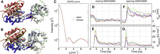
(A) Snapshot of LBP in open state and (B) near-closed state during SWAXS-driven MD. Imposed SWAXS-derived forces at this simulation time from Cα-atoms (green arrows). (C) Computed SWAXS-curves for open (light green) and closed LBP (red), from 20 to 100-ns segments of equilibrium MD trajectories; these SWAXS curves were used as target curves for SWAXS-driven MD in (D–G). (D and F) Domain separation dsep and (E and G) ESWAXS over time for five closing (D and E) and five opening trajectories (F and G), using parameters of kc = 1000, τ = 1 ns. To see this figure in color, go online.
As a control, we first conducted multiple free simulations of LBP starting from the apo and holo crystal structures. These free simulations sampled their respective open and closed conformations (Fig. 2 A, green/red dots), but did not sample any complete transitions within 100 ns, regardless of the presence or absence of ligand at the binding interface (Fig. S3). This lack of sampling shows that MD simulations alone would be insufficient to predict the apo state of LBP given only the holo structure, or vice versa. Such problems are common, because most biologically relevant transitions occur on time scales inaccessible to MD.
Figure 2.
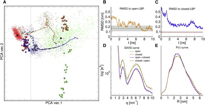
(A) PCA of unbiased simulations, SWAXS-driven MD, and rigid-body modeling. PCA vectors 1 and 2 approximately correspond to opening and twisting motions. (Red and green dots) Ensembles of unbiased simulations of closed (red) and open (green) LBP, which were used to compute the target SWAXS curves for SWAXS-driven MD (Fig. 1C). (Black dots) Cluster center of closed and open ensembles used for the RMSD analysis in subplots (B and C). (Orange/blue dots) Conformations during SWAXS-driven MD in the opening (orange) and closing simulation (blue). (Orange and blue lines) To guide the eye, smoothed SWAXS-driven trajectories are shown. (Black arrows) Forces derived from ESWAXS, mainly acting along the opening motion. (Plus and cross symbols) Conformations predicted by rigid-body modeling, using SASREF. Analogous colors to SWAXS-driven MD are adopted: (red) control SASREF runs of holo-LBP targeting holo spectra (holo → holo); (green) apo-LBP targeting apo spectra (apo → apo); (orange) holo → apo; and (blue) apo → holo. (B and C) SWAXS-driven trajectories in (A) plotted by RMSD to the cluster-center conformation. For reference, the RMSD of the target ensembles are indicated (green/red dashed lines) with errors (gray) shown in background. (D) Scattering-curves of SWAXS-driven trajectories at t = 10 ns, with τ = 1 ns, as compared to the target curves from Fig. 1C. (Orange and green curves) For clarity, these curves have been vertically offset. (E) P(r) curves of the spectra in (D) computed with GNOM (55). See the Supporting Material for details. To see this figure in color, go online.
SWAXS-driven MD using a nonweighted SWAXS potential
In the following, we show rapid conformational transition of LBP by using information from computationally generated SWAXS curves. SWAXS curves of LBP were computed from apo and holo ensembles sampled in free simulations (Fig. 2, green/red dots), producing the target curves in Fig. 1 C. The radius of gyration Rgyr of these curves agree with SAXS measurements of a homolog LIVBP (78% identity), although it is significantly smaller than crystallographic values (Table 1). This suggests that our calculated LBP SWAXS curves are consistent with experimental solution conditions.
Table 1.
Radius of gyration of apo and Phe-bound LBP
| Structures | Crystallography | Simulation | LIVBP (SAXS) |
|---|---|---|---|
| Apo | 2.80 | 2.28 | 2.33 ± 0.02 |
| Holo | 2.33 | 2.19 | 2.23 ± 0.02 |
Multiple SWAXS-driven MD simulations were started from closed LBP and targeting the SWAXS curve of open LBP, and vice versa. SWAXS-driven MD based on a nonweighted coupling potential (Eq. 2) is presented in the following, and simulations based on a weighted potential (Eq. 3) are discussed further below. As shown in Fig. 1, D–G, coupling of simulations to target SWAXS curves of open and closed LBP induced rapid changes in the domain separation dsep toward target values. At the end of the transition, the protein exhibited a reasonably low root-mean-square deviation (RMSD) to the cluster center of the open and closed ensembles, which were used compute the target SWAXS curves (Fig. 2, B and C). In addition, and as expected, the SWAXS curves and pair distribution functions P(r) computed from the final frames of the SWAXS-driven MD are in close agreement to the target curves (Fig. 2, D and E). A moderate ESWAXS bias of 15–30 kJ/mol (Fig. 1, E and G) was sufficient to trigger rapid transitions, which was followed by an equilibration toward the target state within 10 ns (Fig. 2 A). Decomposing ESWAXS into contributions from different scattering vectors q demonstrate that transitions were primarily driven by the difference signal at 2 nm−1 (Fig. S4). We note that during the opening transition (Fig. 1 F), some overcompensation occurred due to memory effects (Eq. 6), but such effects can be lessened by reducing the constant kc at the cost of slower transitions (Fig. S5).
The driving forces for the conformational transitions are further analyzed Figs. 2 A and 3, which visualize transition pathways and ESWAXS, respectively, along the eigenvectors from a principal component analysis (PCA). As shown in Fig. 2 A, we observed a further relaxation of LBP along a twisting motion after the equilibration of ESWAXS, both after opening and closing transitions (orange and blue curves, respectively). This twisting motion is almost perpendicular to SWAXS-derived forces (arrows in Fig. 2), suggesting that the MD force field is primarily responsible for these twisting relaxations, and not the SWAXS data. The ESWAXS landscape of LBP in analyzed in detail in Fig. 3, showing a large gradient of ESWAXS along the opening/closing motion. In contrast, ESWAXS is nearly invariant along the twisting motion, suggesting that only the MD force field can discriminate between states of different twist. Taken together, we find that the MD force field is required to complement the SWAXS signals in order to characterize the LBP solution states, while the SWAXS signals trigger the conformal transitions along the opening motion within the accessible simulation time.
Figure 3.
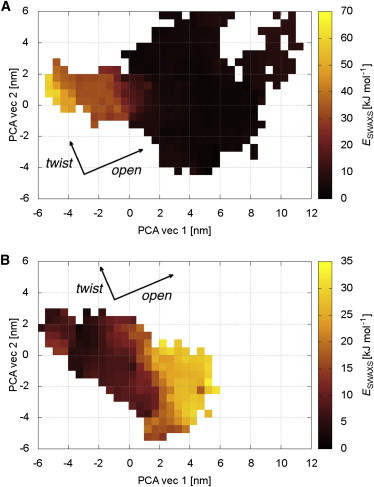
Energy landscape of ESWAXS during SWAXS-driven simulations of LBP, binned along the first two PCA eigenvectors (see Fig. 2). The analysis demonstrates that the SWAXS data mainly encodes structural transitions along the opening motion. Transitions along the twisting motion are not coupled by SWAXS restraints, and hence require sampling under the influence of the MD force field. (A) Simulations targeting open LBP. (B) Simulations targeting closed LBP. Data was collected from the equilibration period (4–10 ns, t > 4τ). In order to sample the ESWAXS landscape exhaustively, a total of 30 trajectories were simulated for each figure using coupling strengths of kc = 100, 300, and 1000. ESWAXS was scaled to match ESWAXS simulations using kc = 1000. To see this figure in color, go online.
Comparison to rigid-body modeling
The role of the applied force field was further investigated by comparing the SWAXS-driven MD to rigid-body modeling, as, for instance, implemented in the SASREF tool of the ATSAS software package (42). In contrast to atomistic MD simulations, SASREF employs rigid-body motions to minimize the intensity difference with the experiment, and further ranks complexes using a knowledge-based scoring function over residue-residue contacts. Details of our ATSAS modeling are given in the Supporting Material. To compare SWAXS-driven MD and ATSAS approaches, the final structures from rigid-body modeling are shown as plus-symbols in the PCA projection in Fig. 2 A, and their RMSDs to cluster-center structures are shown in Table 2.
Table 2.
LBP RMSD versus cluster-center structures, for conformations determined by ATSAS rigid-body modeling or SWAXS-driven MD
| Description | RMSDapo | RMSDholo |
|---|---|---|
| ATSAS fitting | ||
| Apo → apo | 4.40 ± 1.09 | 6.29 ± 0.77 |
| Holo → apo | 3.13 ± 0.24 | 5.08 ± 0.16 |
| Holo → holo | 3.69 ± 0.22 | 2.34 ± 0.30 |
| Apo → holo | 3.93 ± 0.85 | 2.77 ± 1.58 |
| SWAXS-driven MD | ||
| Apo → apo | 1.47 ± 0.34 | 4.43 ± 0.44 |
| Holo → apo | 2.23 ± 0.59 | 4.33 ± 0.65 |
| Holo → holo | 4.41 ± 0.62 | 1.38 ± 0.34 |
| Apo → holo | 3.35 ± 0.37 | 2.08 ± 0.61 |
ATSAS models were built using N- and C-terminal domains of the apo- and holo-LBP crystal structures as rigid bodies, and targeting the ensemble curves in Fig. 1C. SWAXS-driven MD values obtained by averaging the last nanosecond of five independent simulations, conducted at force constant kc = 1000. See the Supporting Material for details.
We found consistently smaller RMSD of LBP structures derived by SWAXS-driven MD, as compared to rigid-body modeling. In particular, a large spread of ATSAS apo-LBP models along the second PCA vector is seen, loosely corresponding to the twisting motion found in SWAXS-driven MD (green plus symbols in Fig. 2 A). This suggests that ATSAS modeling lacks information necessary to refine a correct twist between the N- and C-terminal domains, despite additional distance constraints. In comparison, holo-LBP models found by ATSAS are of comparable accuracy to those found by SWAXS-driven MD, implying that both ATSAS- and SWAXS-driven MD possess sufficient information here. We further rationalize this difference from the ESWAXS landscape of apo- and holo-LBP (Fig. 3). While the holo-LBP state is relatively well defined in ESWAXS, the apo-LBP landscape is almost flat along the twisting motion. This explains the large potential distribution in ATSAS modeling, while SWAXS-driven MD additionally benefits from the information provided by the MD force field.
SWAXS-driven MD using an uncertainty-weighted SWAXS potential
In order to explicitly account for uncertainties of I(q), we carried out SWAXS-driven MD of LBP using the weighted SWAXS potential of Eq. 3. Because we here coupled the simulations to calculated SWAXS curves, we assumed that the relative experimental error linearly increases with q, resembling the errors of the experimental data we used in a previous study (26). The uncertainties σe(q), σbuf(q), and σc(q) are shown in Fig. S6, demonstrating that, for the LBP model, the uncertainty of the buffer density dominates at low q, while the experimental errors dominates at high q. Hence, disregarding any of these error contributions would lead to a significant underestimate of the overall uncertainty for certain q ranges. The dsep, ESWAXS, and the PCA analysis of multiple transitions are visualized in Fig. S7. These transitions resemble those from the nonweighted SWAXS-driven MD, suggesting that the functional form for ESWAXS plays only a minor role for LBP. For simplicity, we therefore applied the nonweighted coupling scheme for the remainder of the article.
ATCase
ATCase is the first member of the pyrimidine synthesis pathway. It is composed of 12 subunits with three regulatory dimers surrounding a pair of catalytic trimers (Fig. 4). Two conformational states T and R corresponding to low and high activities are known, related by a concerted transition that is triggered by binding of a cosubstrate and further regulated by nucleotide binding (37,43). Whereas the crystallographic T state is compatible with SAXS data of T, Fetler and Vachette (37) and Svergun et al. (44) noticed that the solution state of R is more expanded as compared to the crystal structure of R (here termed Rcryst). Hence, we used SWAXS-driven MD to characterize the solution state of R, based on published experimental SAXS data (37).
Figure 4.
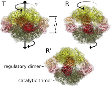
Snapshots of T- (top left), R- (top right), and R′-ATCase, viewed from one of the three regulatory dimers (orange and red; left, center and right domains) connecting the opposing catalytic trimers (yellow and tan; top and bottom domains). (Black arrows) Concerted motion connecting T ↔ R ↔ R′, involving an expansion along the trimer separation d and corotation of trimers in ϕ. To see this figure in color, go online.
To begin, we conducted conventional simulations starting at T and Rcryst. SAXS curves computed from these simulations are compared to experimental data in Fig. 5 A, and conformational transitions are quantified in Fig. 5 B using the center-of-mass distance d as well as the rotational angle ϕ between the two trimers (Fig. 4). Simulations starting at T were highly stable, and SAXS curves computed from the simulations favorably agree with available SAXS data (Fig. 5 A, red solid line versus red/orange crosses). In contrast, simulations that are restrained to Rcryst are incompatible with experimental SAXS data, suggesting that the crystal lattice stabilized a compact conformation (Fig. 5 A, purple solid line versus green/blue crosses). Indeed, ATCase in free simulations starting from Rcryst spontaneously expand, coupled to relative rotation of the two trimers (Fig. 5 B, green). That transition leads to an improved agreement with SAXS data of the R state at q ≈ 0.8 mm−1 (Fig. 5 A, green curve). However, none of our equilibrium simulations could explain the difference between the R and T curves at q ≈ 2 mm−1 (Fig. 5 A). These findings suggest that our free MD simulations did not fully describe the solution R state, further emphasized by variations observed between individual simulation trajectories.
Figure 5.
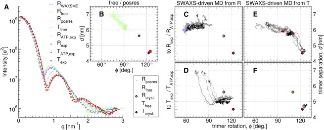
(A) SAXS curves of free ATCase simulations starting from crystallographic Tcryst (solid dark-red) or crystallographic Rcryst (solid light-green), and position-restrained to Rcryst (dotted purple). (Blue dashed line) SWAXS-driven MD targeting the experimental curve Rexp. The ensembles used to compute solid and dashed curves in (A) are shown as dots of the same colors in subplots (B) and (C). Experimental curves (37), shown as pluses/crosses, were fitted with function Ifit = fIe + c, as described previously (26). Experimental curves are shown for both ATP-bound (green/tan pluses) and ATP-free states (blue/red crosses). (B) Unbiased and position-restrained ensembles of (A) plotted along relative catalytic trimer rotation ϕ and separation d. Legend shown below the plot. (Diamonds) Starting crystallographic positions (Tcryst and Rcryst); (dots) simulation frames. Note that the position-restrained R ensemble (Rposres, purple dots) is hardly visible behind the (green) diamond. (C–F) SWAXS-driven MD simulations; (C) 6 × R → R, (D) 6 × R → T, (E) 6 × T → R, and (F) 5 × T → T. (Gray lines) Simulations coupled to ATP-bound SAXS curves RATP,exp/TATP,exp. (Black lines) Simulations coupled to ATP-unbound SAXS curves RexpTexp. (Blue dashed line) Ensemble from SWAXS-driven MD targeting Rexp used to compute the (blue dashed) SAXS curve in (A). (Red dashed line) Control simulation targeting a computed unbiased R-state curves. (Circles) Last frames. Trajectories span 20–23 ns, using parameters of τ = 1 ns and kc = 500. To see this figure in color, go online.
Results from SWAXS-driven MD simulations are presented in Fig. 5, C–F, starting from final frames of free R or free T simulations. Associated I(q) and P(r) curves are shown in Figs. S9 and S10. As controls, T → T simulations are stable, and R → T simulations reach a closed position near T (Fig. 5, D and F). Here we find that further closure is prevented by flexible loops of the catalytic trimer, whose rearrangement is necessary for reforming the T-interface. Because such details are not encoded in the SAXS signal, longer simulations or enhanced sampling techniques would be required to fully reach the T state.
Simulations coupled to the R curve rapidly open and consistently suggest that the trimers are on average separated by ∼6.3 nm in solution, ∼0.7 nm more as compared to Rcryst (Fig. 5, C and E). Compared to free simulations and previous modeling efforts, however, the SWAXS-driven simulations suggest ATCase conformations characterized by a further trimer rotation, corresponding to smaller ϕ (Fig. 4, R′). We note that after releasing the SWAXS-derived potential, those simulations partly returned to larger ϕ angles, suggesting that the simulations were not yet able to accommodate a stable rotated structure within the simulation time of ∼20 ns (Fig. S9).
To identify the subset of experimental scattering data that encourages rotated R′-ATCase, we conducted additional SWAXS-driven MD with restricted coupling ranges. The two main features of R-SAXS were coupled to individual simulations: 1) ∼0.8 nm−1 or 2) at 2 nm−1 (Fig. S8). Coupling only to the 0.8 nm−1-range fixed the trimer separation near 6.3 nm but induced no additional rotation, suggesting that this feature mainly encodes the trimer separation. In contrast, coupling to the feature at 2.0 nm−1 was found to influence trimer rotations ϕ, yielding R′-conformers similar to those found by the coupling to the entire q range. These findings further suggest that highly rotated conformers are significantly populated in the solution state of ATCase. More importantly, the analysis demonstrates how SWAXS-driven MD interprets features of a SWAXS curve in terms of specific collective modes of the biomolecule.
Nuclear exportin 1
CRM1 is a nuclear exportin composed of 21 HEAT repeats arranged in a ringlike structure. Its structure-function relationships are complex: crystallographic studies yield a ring-open conformation for the apo form (45), but closed when in complex with cofactors or cargo (46,47). However, cryo-electron microscopy identifies different degrees of openness apo-CRM1 (45). Here, we revisited CRM1 by means of SWAXS-driven MD coupled to experimental SAXS patterns (48), to understand the solution state of apo CRM1.
To test whether MD simulations alone would provide a consistent solution ensemble of CRM1, we first simulated the open apo-CRM1 using two different force fields and salt concentrations (Fig. 6, A and C, Fig. S11). Surprisingly, we observe spontaneous ring-closure under CHARMM22∗ (49) but ring-opening under the AMBER99sb force field (50). Simulations with 100 mM NaCl instead of only counterions exhibited slightly higher ring-open populations, but a significant force-field bias remains. These discrepancies suggest that the energy surface underlying CRM1 conformations is very shallow and, hence, highly sensitive to force-field differences. Furthermore, the SAXS patterns of these distributions suggest that neither distribution correctly reproduced the experimental data (Fig. 6 B).
Figure 6.
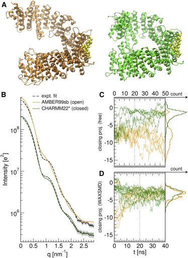
(A) Snapshots of CRM1 simulated with the AMBER99sb (orange, left) and CHARMM22∗ (green, right) force fields, respectively, in a ring-open and ring-closed conformation. (B) Predicted SAXS curves of open (AMBER99sb, lighter orange) and closed (CHARMM22∗, darker green) CRM1 computed from the last 30 ns of the simulations (D); (dashed black line) fitted, smoothed experimental curve; (solid gray) error bars. (C) Display of 50-ns trajectories and last 30-ns histograms of free CRM1 in AMBER99sb (lighter orange) and CHARMM22∗ (darker green), plotted according to the atomic difference vector between open (PDB:4FGV) and closed (PDB:3GJX) CRM1, the same metric as used in Monecke et al. (45) Significant force-field dependence is found. (D) A display of the 40-ns SWAXS-driven MD of CRM1, exhibiting no dependence on the force field. To see this figure in color, go online.
Fig. 6 D presents trajectories of SWAXS-driven MD started from the final frames of free MD simulations. Associated I(q) and P(r) curves are shown in Fig. S12. We find that SWAXS-driven MD suggests an intermediate average solution state of CRM1, which is more open than predicted by CHARMM22∗ but more closed than predicted by AMBER99sb. The SAXS curve of the refined ensemble (Fig. S13 B) resembles that of the target curve. Only small deviations at very small angles remain, which we did not couple to the simulations, in order to exclude concentration-dependent experimental artifacts. We further verified the refinement by performing the χ2free analysis suggested by Rambo and Tainer (12) over individual SWAXS-driven trajectories (Fig. S14). Although the SAXS curve for the total ensemble of 10 replica is in good agreement to experiment, we find significant variations in individual χ2free, suggesting that the MD force field imposed tight restraints on possible conformations, and that the refinement is far from overfitting.
The alignment of ring-geometries to an intermediate conformation, however, does not exclude the possibility of a more heterogeneous open/closed solution ensemble. We therefore modeled the CRM1 ensemble as a linear combination of open and closed states from CHARMM22∗ simulations, and evaluated the fits with our χ2 metric (Eq. S1 in the Supporting Material) and the χ2free metric (Fig. S1). We found that our χ-metric reports an optimum ratio of 60% open/40% closed CRM1, while the χ2free-metric reports ∼75% open populations. Although the exact ratios differ, both are comparable to 2:1, suggested by cryo-electron microscopy experiments (45).
Thus, the ensemble-averaged SAXS data encodes the average solution structure, but it is in this case insufficient to determine the variance of the open/closed distribution. In order to interpret such heterogeneous ensembles, it will be highly interesting to couple multiple replicas of a simulation to one ensemble-averaged SWAXS curve, thereby also refining the relative weights of the replicas. Because that approach will require additional care to avoid overfitting, we leave that extension to a future study.
Conclusions
Many proteins carry out their biological function via conformational transitions. High-resolution crystallographic structures are frequently only available for one state, such as a ground state or a holo state, whereas SWAXS data may be available for the complete conformational cycle. However, due to the large number of degrees of freedom, the interpretation of the SWAXS data in terms of conformational transitions would be ill defined without prior physical knowledge. Starting from related crystallographic structures, we here employed explicit-solvent MD simulations to refine structures against SWAXS curves. The simulations provide an accurate prior distribution of accessible conformational states, and they are not subject to the restriction associated with rigid-body MD or normal mode fitting, which were previously used to refine structures against SAXS data (51,52). The commitment to explicit solvent and atomistic models of scattering also allows the accurate calculation of curves at wide angles (25,26,33). The explicit-solvent calculations require, apart from an overall scaling factor for the intensities, only one additional fitting parameter that accounts for uncertainties in the buffer subtraction. In particular, and in contrast to implicit solvent calculations, they do not require fitting of the solvation layer or excluded solvent, thus retaining the ability to differentiate small alterations in protein structure (26).
The three biomolecular systems presented here highlight the complementarity between SWAXS and MD techniques. As frequently found for biomolecular systems, we observed in all three examples that conventional MD simulations were insufficient to fully characterize the solution states of the proteins, due to limited sampling (LBP and ATCase) or force-field inaccuracies (CRM1). Incorporating SWAXS curves into the simulation reduced a possible force-field bias and accelerated conformational transitions without prior knowledge of possible reaction paths. In particular, the algorithm does not push the biomolecule along preselected collective modes such as PCA or normal modes, as would be common for many accelerated MD algorithms. Instead, the information of the SWAXS curve is merely added to the MD force field, and the simulation decides which collective motions are most appropriate to meet both experimental and physical restraints. In turn, during structure refinement, the MD simulation added physical knowledge to the SWAXS curves, thereby 1) restricting the refinement to physically realistic motions and 2) allowing further relaxation along collective motions that are not encoded in the SWAXS curve.
We validated SWAXS-driven MD using two different metrics of the coupling potential. First, a nonweighted metric on a logarithmic scale was applied (Eq. 2), which is conceptually simple, numerically stable and, hence, suitable from a practical perspective. In particular, this metric is rather insensitive to poor buffer matching, which is a common problem in SWAXS experiments, and it imposes reasonable statistical weights on small versus wide-angle data. Second, a more rigorous coupling metric was implemented by imposing the overall uncertainties as inverse weights, given by experimental σe and calculated σc statistical errors as well as a systematic error σbuf from the buffer subtraction (Eqs. 3 and 4). We found incorporating σbuf to be crucial for SWAXS-driven MD, in order to account for cases of poor buffer matching. Ignoring σbuf and instead applying σe alone would impose spuriously high weights to small q, which frequently lead to numerical instabilities during SWAXS-driven simulations (not shown). The error σbuf, on the contrary, dominates the overall error at small q, thereby reducing those weights to physically justified values. As a consequence, the uncertainty-weighted SWAXS-driven MD simulations were numerically stable, capable of interpreting intensity variations over the entire q range. However, finding a rigorous procedure to distribute the weights along q may require more research.
Our implementation of SWAXS-driven MD uses certain heuristic parameters to achieve efficient sampling: coupling strength kc, and memory time τ. Their optimal choices depend upon the energy landscape of the system, and we noted above that adopting a constant kc does risk temporary overcompensation, as observed for LBP (Fig. 1 F). We are investigating possibilities for adaptive coupling schemes that would avoid such artifacts arising from an ad hoc selection of these parameters. For instance, it will be interesting to test the effect of τ on the heterogeneity of the refined ensemble, and to compare it with the protein flexibility as quantified from Kratky and Porod-Debye plots (53). In addition, the calculations shown here required us to fit experimental curves against calculated curves before starting the SWAXS-driven MD (Eq. S1 in the Supporting Material), in order to remove some of the uncertainty from poor buffer matching. In a future study, we instead aim to include the fitting step explicitly into the coupling scheme, if possible by using an inferential (Bayesian) approach (54). In addition, future efforts aim to render the methods shown here easily accessible to researchers that have little computational background. We note that SWAXS-driven MD is applicable to neutron scattering data, and it can be straightforwardly generalized to more heterogeneous ensembles by coupling multiple replicas of the biomolecule simultaneously to a target SWAXS curve. We expect SWAXS-driven MD presented here, complemented by such future developments, to become a useful protocol for biomolecular research.
Author Contributions
P.-c.C. and J.S.H. designed and performed research and wrote the article; P.-c.C. analyzed data.
Acknowledgments
We thank T. Monecke, A. Dickmanns, and R. Ficner for the SAXS curve of CRM1; B. Voss and H. Grubmüller for the AMBER99sb simulation system of CRM1; and A. Dickmanns and K. Atkovska for critically reading the article. Computing time by the North-German Supercomputing Alliance is gratefully acknowledged.
This study was supported by the Deutsche Forschungsgemeinschaft (grant No. HU 1971/1-1).
Supporting Material
Supporting Citations
References (56–70) appear in the Supporting Material.
References
- 1.Putnam C.D., Hammel M., Tainer J.A. X-ray solution scattering (SAXS) combined with crystallography and computation: defining accurate macromolecular structures, conformations and assemblies in solution. Q. Rev. Biophys. 2007;40:191–285. doi: 10.1017/S0033583507004635. [DOI] [PubMed] [Google Scholar]
- 2.Graewert M.A., Svergun D.I. Impact and progress in small and wide angle x-ray scattering (SAXS and WAXS) Curr. Opin. Struct. Biol. 2013;23:748–754. doi: 10.1016/j.sbi.2013.06.007. [DOI] [PubMed] [Google Scholar]
- 3.Rodi D.J., Mandava S., Fischetti R.F. Detection of functional ligand-binding events using synchrotron x-ray scattering. J. Biomol. Screen. 2007;12:994–998. doi: 10.1177/1087057107306104. [DOI] [PubMed] [Google Scholar]
- 4.He L., André S., Gabius H.-J. Detection of ligand- and solvent-induced shape alterations of cell-growth-regulatory human lectin galectin-1 in solution by small angle neutron and x-ray scattering. Biophys. J. 2003;85:511–524. doi: 10.1016/S0006-3495(03)74496-8. [DOI] [PMC free article] [PubMed] [Google Scholar]
- 5.Pietri R., Zerbs S., Miller L.M. Biophysical and structural characterization of a sequence-diverse set of solute-binding proteins for aromatic compounds. J. Biol. Chem. 2012;287:23748–23756. doi: 10.1074/jbc.M112.352385. [DOI] [PMC free article] [PubMed] [Google Scholar]
- 6.Mould A.P., Symonds E.J.H., Humphries M.J. Structure of an integrin-ligand complex deduced from solution x-ray scattering and site-directed mutagenesis. J. Biol. Chem. 2003;278:39993–39999. doi: 10.1074/jbc.M304627200. [DOI] [PubMed] [Google Scholar]
- 7.Cammarata M., Levantino M., Ihee H. Tracking the structural dynamics of proteins in solution using time-resolved wide-angle x-ray scattering. Nat. Methods. 2008;5:881–886. doi: 10.1038/nmeth.1255. [DOI] [PMC free article] [PubMed] [Google Scholar]
- 8.Andersson M., Malmerberg E., Neutze R. Structural dynamics of light-driven proton pumps. Structure. 2009;17:1265–1275. doi: 10.1016/j.str.2009.07.007. [DOI] [PubMed] [Google Scholar]
- 9.Ramachandran P.L., Lovett J.E., van Thor J.J. The short-lived signaling state of the photoactive yellow protein photoreceptor revealed by combined structural probes. J. Am. Chem. Soc. 2011;133:9395–9404. doi: 10.1021/ja200617t. [DOI] [PubMed] [Google Scholar]
- 10.Grishaev A., Wu J., Bax A. Refinement of multidomain protein structures by combination of solution small-angle x-ray scattering and NMR data. J. Am. Chem. Soc. 2005;127:16621–16628. doi: 10.1021/ja054342m. [DOI] [PubMed] [Google Scholar]
- 11.Schwieters C.D., Suh J.-Y., Clore G.M. Solution structure of the 128 kDa enzyme I dimer from Escherichia coli and its 146 kDa complex with HPr using residual dipolar couplings and small- and wide-angle x-ray scattering. J. Am. Chem. Soc. 2010;132:13026–13045. doi: 10.1021/ja105485b. [DOI] [PMC free article] [PubMed] [Google Scholar]
- 12.Rambo R.P., Tainer J.A. Accurate assessment of mass, models and resolution by small-angle scattering. Nature. 2013;496:477–481. doi: 10.1038/nature12070. [DOI] [PMC free article] [PubMed] [Google Scholar]
- 13.Schneidman-Duhovny D., Hammel M., Sali A. Macromolecular docking restrained by a small angle x-ray scattering profile. J. Struct. Biol. 2011;173:461–471. doi: 10.1016/j.jsb.2010.09.023. [DOI] [PMC free article] [PubMed] [Google Scholar]
- 14.Karaca E., Bonvin A.M.J.J. On the usefulness of ion-mobility mass spectrometry and SAXS data in scoring docking decoys. Acta Crystallogr. D Biol. Crystallogr. 2013;69:683–694. doi: 10.1107/S0907444913007063. [DOI] [PubMed] [Google Scholar]
- 15.Neutze R., Moffat K. Time-resolved structural studies at synchrotrons and x-ray free electron lasers: opportunities and challenges. Curr. Opin. Struct. Biol. 2012;22:651–659. doi: 10.1016/j.sbi.2012.08.006. [DOI] [PMC free article] [PubMed] [Google Scholar]
- 16.Levantino M., Spilotros A., Cupane A. The Monod-Wyman-Changeux allosteric model accounts for the quaternary transition dynamics in wild type and a recombinant mutant human hemoglobin. Proc. Natl. Acad. Sci. USA. 2012;109:14894–14899. doi: 10.1073/pnas.1205809109. [DOI] [PMC free article] [PubMed] [Google Scholar]
- 17.Bernadó P., Svergun D.I. Structural analysis of intrinsically disordered proteins by small-angle x-ray scattering. Mol. Biosyst. 2012;8:151–167. doi: 10.1039/c1mb05275f. [DOI] [PubMed] [Google Scholar]
- 18.Yang S., Blachowicz L., Roux B. Multidomain assembled states of Hck tyrosine kinase in solution. Proc. Natl. Acad. Sci. USA. 2010;107:15757–15762. doi: 10.1073/pnas.1004569107. [DOI] [PMC free article] [PubMed] [Google Scholar]
- 19.Różycki B., Kim Y.C., Hummer G. SAXS ensemble refinement of ESCRT-III CHMP3 conformational transitions. Structure. 2011;19:109–116. doi: 10.1016/j.str.2010.10.006. [DOI] [PMC free article] [PubMed] [Google Scholar]
- 20.Svergun D., Barberato C., Koch M.H.J. CRYSOL—a program to evaluate x-ray solution scattering of biological macromolecules from atomic coordinates. J. Appl. Cryst. 1995;28:768–773. [Google Scholar]
- 21.Merzel F., Smith J.C. SASSIM: a method for calculating small-angle x-ray and neutron scattering and the associated molecular envelope from explicit-atom models of solvated proteins. Acta Crystallogr. D Biol. Crystallogr. 2002;58:242–249. doi: 10.1107/s0907444901019576. [DOI] [PubMed] [Google Scholar]
- 22.Bardhan J., Park S., Makowski L. SOFTWAXS: a computational tool for modeling wide-angle x-ray solution scattering from biomolecules. J. Appl. Cryst. 2009;42:932–943. doi: 10.1107/S0021889809032919. [DOI] [PMC free article] [PubMed] [Google Scholar]
- 23.Grishaev A., Guo L., Bax A. Improved fitting of solution x-ray scattering data to macromolecular structures and structural ensembles by explicit water modeling. J. Am. Chem. Soc. 2010;132:15484–15486. doi: 10.1021/ja106173n. [DOI] [PMC free article] [PubMed] [Google Scholar]
- 24.Poitevin F., Orland H., Delarue M. AQUASAXS: a web server for computation and fitting of SAXS profiles with non-uniformally hydrated atomic models. Nucleic Acids Res. 2011;39:W184–W189. doi: 10.1093/nar/gkr430. [DOI] [PMC free article] [PubMed] [Google Scholar]
- 25.Köfinger J., Hummer G. Atomic-resolution structural information from scattering experiments on macromolecules in solution. Phys. Rev. E Stat. Nonlin. Soft Matter Phys. 2013;87:052712. doi: 10.1103/PhysRevE.87.052712. [DOI] [PubMed] [Google Scholar]
- 26.Chen P.C., Hub J.S. Validating solution ensembles from molecular dynamics simulation by wide-angle x-ray scattering data. Biophys. J. 2014;107:435–447. doi: 10.1016/j.bpj.2014.06.006. [DOI] [PMC free article] [PubMed] [Google Scholar]
- 27.Rambo R.P., Tainer J.A. Super-resolution in solution x-ray scattering and its applications to structural systems biology. Annu. Rev. Biophys. 2013;42:415–441. doi: 10.1146/annurev-biophys-083012-130301. [DOI] [PubMed] [Google Scholar]
- 28.Brünger A.T., Kuriyan J., Karplus M. Crystallographic R factor refinement by molecular dynamics. Science. 1987;235:458–460. doi: 10.1126/science.235.4787.458. [DOI] [PubMed] [Google Scholar]
- 29.Lange O.F., Lakomek N.-A., de Groot B.L. Recognition dynamics up to microseconds revealed from an RDC-derived ubiquitin ensemble in solution. Science. 2008;320:1471–1475. doi: 10.1126/science.1157092. [DOI] [PubMed] [Google Scholar]
- 30.Trabuco L.G., Villa E., Schulten K. Flexible fitting of atomic structures into electron microscopy maps using molecular dynamics. Structure. 2008;16:673–683. doi: 10.1016/j.str.2008.03.005. [DOI] [PMC free article] [PubMed] [Google Scholar]
- 31.Moore P.B. The effects of thermal disorder on the solution-scattering profiles of macromolecules. Biophys. J. 2014;106:1489–1496. doi: 10.1016/j.bpj.2014.02.016. [DOI] [PMC free article] [PubMed] [Google Scholar]
- 32.Oroguchi T., Ikeguchi M. Effects of ionic strength on SAXS data for proteins revealed by molecular dynamics simulations. J. Chem. Phys. 2011;134:025102. doi: 10.1063/1.3526488. [DOI] [PubMed] [Google Scholar]
- 33.Park S., Bardhan J.P., Makowski L. Simulated x-ray scattering of protein solutions using explicit-solvent models. J. Chem. Phys. 2009;130:134114. doi: 10.1063/1.3099611. [DOI] [PMC free article] [PubMed] [Google Scholar]
- 34.Doyle P.A., Turner P.S. Relativistic Hartree-Fock x-ray and electron scattering factors. Acta Crystallogr. A. 1968;24:390–397. [Google Scholar]
- 35.Sorenson J.M., Hura G., Head-Gordon T. What can x-ray scattering tell us about the radial distribution functions of water? J. Chem. Phys. 2000;113:9149–9161. [Google Scholar]
- 36.Gumerov N.A., Berlin K., Duraiswami R. A hierarchical algorithm for fast Debye summation with applications to small angle scattering. J. Comput. Chem. 2012;33:1981–1996. doi: 10.1002/jcc.23025. [DOI] [PMC free article] [PubMed] [Google Scholar]
- 37.Fetler L., Vachette P. The allosteric activator Mg-ATP modifies the quaternary structure of the R-state of Escherichia coli aspartate transcarbamylase without altering the T↔R equilibrium. J. Mol. Biol. 2001;309:817–832. doi: 10.1006/jmbi.2001.4681. [DOI] [PubMed] [Google Scholar]
- 38.Vestergaard B., Hansen S. Application of Bayesian analysis to indirect Fourier transformation in small-angle scattering. J. Appl. Cryst. 2006;39:797–804. [Google Scholar]
- 39.Hess B., Kutzner C., Lindahl E. GROMACS 4: algorithms for highly efficient, load-balanced, and scalable molecular simulation. J. Chem. Theory Comput. 2008;4:435–447. doi: 10.1021/ct700301q. [DOI] [PubMed] [Google Scholar]
- 40.Olah G.A., Trakhanov S., Quiocho F.A. Leucine/isoleucine/valine-binding protein contracts upon binding of ligand. J. Biol. Chem. 1993;268:16241–16247. [PubMed] [Google Scholar]
- 41.Magnusson U., Salopek-Sondi B., Mowbray S.L. X-ray structures of the leucine-binding protein illustrate conformational changes and the basis of ligand specificity. J. Biol. Chem. 2004;279:8747–8752. doi: 10.1074/jbc.M311890200. [DOI] [PubMed] [Google Scholar]
- 42.Petoukhov M.V., Svergun D.I. Global rigid body modeling of macromolecular complexes against small-angle scattering data. Biophys. J. 2005;89:1237–1250. doi: 10.1529/biophysj.105.064154. [DOI] [PMC free article] [PubMed] [Google Scholar]
- 43.Macol C.P., Tsuruta H., Kantrowitz E.R. Direct structural evidence for a concerted allosteric transition in Escherichia coli aspartate transcarbamylase. Nat. Struct. Biol. 2001;8:423–426. doi: 10.1038/87582. [DOI] [PubMed] [Google Scholar]
- 44.Svergun D.I., Barberato C., Vachette P. Large differences are observed between the crystal and solution quaternary structures of allosteric aspartate transcarbamylase in the R state. Proteins. 1997;27:110–117. [PubMed] [Google Scholar]
- 45.Monecke T., Haselbach D., Ficner R. Structural basis for cooperativity of CRM1 export complex formation. Proc. Natl. Acad. Sci. USA. 2013;110:960–965. doi: 10.1073/pnas.1215214110. [DOI] [PMC free article] [PubMed] [Google Scholar]
- 46.Monecke T., Güttler T., Ficner R. Crystal structure of the nuclear export receptor CRM1 in complex with Snurportin1 and RanGTP. Science. 2009;324:1087–1091. doi: 10.1126/science.1173388. [DOI] [PubMed] [Google Scholar]
- 47.Dong X., Biswas A., Chook Y.M. Structural basis for leucine-rich nuclear export signal recognition by CRM1. Nature. 2009;458:1136–1141. doi: 10.1038/nature07975. [DOI] [PMC free article] [PubMed] [Google Scholar]
- 48.Dölker N., Blanchet C.E., Dickmanns A. Structural determinants and mechanism of mammalian CRM1 allostery. Structure. 2013;21:1350–1360. doi: 10.1016/j.str.2013.05.015. [DOI] [PubMed] [Google Scholar]
- 49.Piana S., Lindorff-Larsen K., Shaw D.E. How robust are protein folding simulations with respect to force field parameterization? Biophys. J. 2011;100:L47–L49. doi: 10.1016/j.bpj.2011.03.051. [DOI] [PMC free article] [PubMed] [Google Scholar]
- 50.Hornak V., Abel R., Simmerling C. Comparison of multiple AMBER force fields and development of improved protein backbone parameters. Proteins. 2006;65:712–725. doi: 10.1002/prot.21123. [DOI] [PMC free article] [PubMed] [Google Scholar]
- 51.Gorba C., Miyashita O., Tama F. Normal-mode flexible fitting of high-resolution structure of biological molecules toward one-dimensional low-resolution data. Biophys. J. 2008;94:1589–1599. doi: 10.1529/biophysj.107.122218. [DOI] [PMC free article] [PubMed] [Google Scholar]
- 52.Zheng W., Tekpinar M. Accurate flexible fitting of high-resolution protein structures to small-angle x-ray scattering data using a coarse-grained model with implicit hydration shell. Biophys. J. 2011;101:2981–2991. doi: 10.1016/j.bpj.2011.11.003. [DOI] [PMC free article] [PubMed] [Google Scholar]
- 53.Rambo R.P., Tainer J.A. Characterizing flexible and intrinsically unstructured biological macromolecules by SAS using the Porod-Debye law. Biopolymers. 2011;95:559–571. doi: 10.1002/bip.21638. [DOI] [PMC free article] [PubMed] [Google Scholar]
- 54.Rieping W., Habeck M., Nilges M. Inferential structure determination. Science. 2005;309:303–306. doi: 10.1126/science.1110428. [DOI] [PubMed] [Google Scholar]
- 55.Svergun D.I. Determination of the regularization parameter in indirect-transform methods using perceptual criteria. J. Appl. Cryst. 1992;25:495–503. [Google Scholar]
- 56.Wang J., Stieglitz K.A., Kantrowitz E.R. Structural basis for ordered substrate binding and cooperativity in aspartate transcarbamylase. Proc. Natl. Acad. Sci. USA. 2005;102:8881–8886. doi: 10.1073/pnas.0503742102. [DOI] [PMC free article] [PubMed] [Google Scholar]
- 57.Gouaux J.E., Stevens R.C., Lipscomb W.N. Crystal structures of aspartate carbamoyltransferase ligated with phosphonoacetamide, malonate, and CTP or ATP at 2.8-Å resolution and neutral pH. Biochemistry. 1990;29:7702–7715. doi: 10.1021/bi00485a020. [DOI] [PubMed] [Google Scholar]
- 58.Mandell D.J., Coutsias E.A., Kortemme T. Sub-Ångstrom accuracy in protein loop reconstruction by robotics-inspired conformational sampling. Nat. Methods. 2009;6:551–552. doi: 10.1038/nmeth0809-551. [DOI] [PMC free article] [PubMed] [Google Scholar]
- 59.Brooks B.R., Brooks C.L., 3rd, Karplus M. CHARMM: the biomolecular simulation program. J. Comput. Chem. 2009;30:1545–1614. doi: 10.1002/jcc.21287. [DOI] [PMC free article] [PubMed] [Google Scholar]
- 60.Bjelkmar P., Larsson P., Lindahl E. Implementation of the CHARMM force field in GROMACS: analysis of protein stability effects from correction maps, virtual interaction sites, and water models. J. Chem. Theory Comput. 2010;6:459–466. doi: 10.1021/ct900549r. [DOI] [PubMed] [Google Scholar]
- 61.Jorgensen W.L., Chandrasekhar J., Klein M.L. Comparison of simple potential functions for simulating liquid water. J. Chem. Phys. 1983;79:926–935. [Google Scholar]
- 62.Essmann U., Perera L., Pedersen L.G. A smooth particle mesh Ewald method. J. Chem. Phys. 1995;103:8577–8593. [Google Scholar]
- 63.Miyamoto S., Kollman P.A. SETTLE: an analytical version of the SHAKE and RATTLE algorithm for rigid water models. J. Comput. Chem. 1992;13:952–962. [Google Scholar]
- 64.Hess B. P-LINCS: a parallel linear constraint solver for molecular simulation. J. Chem. Theory Comput. 2008;4:116–122. doi: 10.1021/ct700200b. [DOI] [PubMed] [Google Scholar]
- 65.Feenstra K.A., Hess B., Berendsen H.J.C. Improving efficiency of large time-scale molecular dynamics simulations of hydrogen-rich systems. J. Comput. Chem. 1999;20:786–798. doi: 10.1002/(SICI)1096-987X(199906)20:8<786::AID-JCC5>3.0.CO;2-B. [DOI] [PubMed] [Google Scholar]
- 66.Parrinello M., Rahman A. Polymorphic transitions in single crystals: a new molecular dynamics method. J. Appl. Phys. 1981;52:7182–7190. [Google Scholar]
- 67.Berendsen H.J.C., Postma J.P.M., Haak J.R. Molecular dynamics with coupling to an external bath. J. Chem. Phys. 1984;81:3684–3690. [Google Scholar]
- 68.Bussi G., Donadio D., Parrinello M. Canonical sampling through velocity rescaling. J. Chem. Phys. 2007;126:014101. doi: 10.1063/1.2408420. [DOI] [PubMed] [Google Scholar]
- 69.Hoover W.G. Canonical dynamics: equilibrium phase-space distributions. Phys. Rev. A. 1985;31:1695–1697. doi: 10.1103/physreva.31.1695. [DOI] [PubMed] [Google Scholar]
- 70.van Gunsteren W.F., Berendsen H.J.C. A leap-frog algorithm for stochastic dynamics. Mol. Simul. 1988;1:173–185. [Google Scholar]
Associated Data
This section collects any data citations, data availability statements, or supplementary materials included in this article.