Deformation-Invariant Sparse Coding for Modeling Spatial Variability of Functional Patterns in the Brain

Abstract

For a given cognitive task such as language processing, the location of corresponding functional regions in the brain may vary across subjects relative to anatomy. We present a probabilistic generative model that accounts for such variability as observed in fMRI data. We relate our approach to sparse coding that estimates a basis consisting of functional regions in the brain. Individual fMRI data is represented as a weighted sum of these functional regions that undergo deformations. We demonstrate the proposed method on a language fMRI study. Our method identified activation regions that agree with known literature on language processing and established correspondences among activation regions across subjects, producing more robust group-level effects than anatomical alignment alone.

1 Introduction

Spatial variability of activation patterns in the brain poses significant challenges to finding functional correspondences across subjects. This variability results in misalignment of individual subjects' activations in an anatomically-normalized space. Consequently, the standard approach of averaging activations in such a space for group analysis sometimes fails to identify functional regions that are spatially variable across individuals, e.g., regions for higher-order tasks such as language processing.

Recent work addresses this variability in different ways [5,6,9]. Thirion et al. [6] identify contiguous regions, or parcels, of functional activation at the subject level and then find parcel correspondences across subjects. While this approach yields reproducible activation regions and provides spatial correspondences across subjects, its bottom-up, rule-based nature does not incorporate a notion of a group template while finding the correspondences. Instead, it builds a group template as a post-processing step. As such, the model lacks a clear group-level interpretation of the estimated parcels. In contrast, Xu et al. [9] use a spatial point process in a hierarchical Bayesian model to describe functional activation regions. Their formulation accounts for variable shape of activation regions and has an intuitive interpretation of group-level activations. However, since the model represents shapes using Gaussian mixture models, functional regions of complex shape could require a large number of Gaussian components. Lastly, Sabuncu et al. [5] sidestep finding functional region correspondences altogether by estimating voxel-wise correspondences through groupwise registration of functional activation maps from different subjects. This approach does not explicitly model functional regions.

We propose a novel way to characterize spatial variability of functional regions that combines ideas from [5,6,9]. We model each subject's activation map as a weighted sum of group-level functional activation parcels that undergo a subject-specific deformation. Our contributions are twofold. First, similar to Xu et al. [9], we define a hierarchical generative model, but instead of using a Gaussian mixture model to represent shapes, we represent each parcel as an image, which allows for complex shapes. By explicitly modeling parcels, our model yields parcel correspondences across subjects, similar to [6]. Second, we assume that the template regions can deform to account for spatial variability of activation regions across subjects. This involves using groupwise registration similar to [5] that is guided by estimated group-level functional activation regions. We perform inference within the proposed model using a variant of the expectation-maximization (EM) algorithm [1] and illustrate our method on the language system, which is known to have significant functional variability [3].

2 Model

We let I = {I₁, I₂,…, I_N} be the N observed images, I_n ∈ ℝ^|Ω| be the activation map for subject n (1 ≤ n ≤ N), and Ω be the set of voxels. We assume that a dictionary of K images D = {D₁, D₂, …, D_K} generates the observed images I. Importantly, each dictionary element corresponds to a group-level parcel. We treat the dictionary size K as a fixed constant; various model selection methods can be used to select K.

We assume that each observed image I_n is generated i.i.d. as follows. First, we draw weight vector w_n ∈ ℝ^K where each scalar entry w_nk is independently sampled from distribution p_w(·; θ_k). Then, we construct pre-image $J_n={\sum }_{k=1}^K{w}_{nk}{D}_k$. The observed image $I_n=J_n\circ {\Phi }_n^{-1}+{\epsilon }_n$ is the result of applying invertible deformation Φ_n to pre-image J_n and adding white Gaussian noise ε_n with variance σ². This process defines the joint probability distribution over the weight vector and observed image for a specific subject:

$$p(I_n,w_n|{\Phi }_n,\mathit{D};\mathit{\theta },{\sigma }^2)=\prod _{k=1}^K{p}_w(w_{nk};{\theta }_k)\prod _{x\in \Omega }\mathcal{N}(I_n(x);\sum _{k=1}^K{w}_{nk}{D}_k({\Phi }_n^{-1}(x)),{\sigma }^2),$$ (1)

where θ = {θ₁, θ₂, …, θ_K}. We aim to infer dictionary D and each deformation Φ_n so that for future experiments performed on the same subjects, we can treat the dictionary and subject-specific deformations as fixed and just estimate the contribution of each dictionary element. By introducing group-level parcels as dictionary elements, the model implicitly contains parcel correspondences since it suffices to look at where a particular dictionary element appears in each subject. Furthermore, each subject need not have all dictionary elements present.

Model Parameters

We treat each deformation Φ_n as a random parameter with prior distribution p_Φ(·), which can also be viewed as regularizing each deformation to prevent overfitting. Choice of the deformation prior allows us to leverage existing image registration algorithms. To prevent spatial drift of the dictionary elements, we constrain the average of the subject-specific deformations, defined as Φ₁ ○ Φ₂ ○ … ○ Φ_N, to be identity:

$$p(\mathit{\Phi })=\prod _{n=1}^N{p}_{\Phi }({\Phi }_n)\cdot 1\{{\Phi }_1\circ \cdots \circ {\Phi }_N=\text{Id}\},$$ (2)

where Φ = {Φ₁, …, Φ_N} and 1{·} is the indicator function that equals 1 when its argument is true and equals 0 otherwise.

We also treat each dictionary element D_k as a random parameter. To resolve an inherent degeneracy where scaling the intensity of dictionary element D_k by constant c and scaling w_nk by 1/c for all n results in the same observed images I, we choose to constrain each dictionary element D_k to have bounded ℓ₂ norm: ‖D_k‖₂ ≤ 1. To encourage sparsity and smoothness, we introduce ℓ₁ and MRF penalties. To constrain each dictionary element to be a parcel, we require each D_k to be a contiguous, unimodal image. Formally,

$$p(D_k;\lambda ,\gamma )\propto exp\{-\lambda \sum _{x\in \Omega }|D_k(x)|-\frac{\gamma }{2}\sum _{x\in \Omega }\sum _{y\in \mathcal{N}(x)}{(D_k(y)-D_k(x))}^2\}\cdot 1\{D_k\text{is a contiguous},\text{unimodal image}\},$$ (3)

where hyperparameters λ and γ are positive constants, and (x) denotes the neighborhood of voxel x.

Other model parameters are treated as non-random: θ parameterizes distribution p_w(·; θ_k) for each k, and σ² is the variance of the Gaussian noise. We use MAP estimation for D and Φ and ML estimation for θ and σ² whereas hyperparameters λ and γ are currently hand-tuned.

For our experiments, we place independent exponential priors on each component of weight vector w_n and use diffeomorphic Demons registration [8] to estimate deformations Φ. In particular, we choose p_w(w_nk; θ_k) = θ_ke^−θ_kw_nk, where w_nk ≥ 0 and θ_k > 0. Moreover, we define p_Φ(Φ_n) ∝ exp{−Reg(Φ_n)}, where Reg(·) is the Demons registration regularization function [8]. Combining these distributions over weights w = {w₁, …, w_N} and deformations Φ with equations (1), (2), and (3), we obtain the full joint distribution:

$$p(\mathit{I},\mathit{w},\mathit{\Phi },\mathit{D};\mathit{\theta },{\sigma }^2)\propto \prod _{n=1}^N\{exp\{-\text{Reg}({\Phi }_n)\}\prod _{k=1}^K{e}^{-{\theta }_k{w}_{nk}}\prod _{x\in \Omega }\mathcal{N}(I_n(x);\sum _{k=1}^K{w}_{nk}{D}_k({\Phi }_n^{-1}(x)),{\sigma }^2\left)\right\}\cdot \prod _{k=1}^{K}exp\{-\lambda \sum _{x\in \Omega }|D_k(x)|-\frac{\gamma }{2}\sum _{x\in \Omega }\sum _{y\in \mathcal{N}(x)}{(D_k(y)-D_k(x))}^2\},$$ (4)

where weights w_nk's are non-negative, average deformation Φ₁ ○ … ○ Φ_N is identity, and each D_k is contiguous and unimodal with ‖D_k‖₂ ≤ 1.

Relation to Sparse Coding

With a heavy-tailed prior p_w concentrated at 0 and no deformations (i.e., deformations are identity), our model becomes equivalent to sparse coding [4]. We extend sparse coding by allowing dictionary elements to undergo subject-specific deformations. In contrast to previous dictionary learning approaches that assume perfect spatial correspondences (e.g., Varoquaux et al. [7]), we estimate jointly a set of deformations Φ and the distribution for weight vectors w in addition to learning the dictionary elements. Effectively, we recover dictionary elements invariant to “small” deformations, where the “size” of a deformation is governed by the deformation prior.

Parameter Estimation

We use a variant¹ of the EM algorithm [1] to estimate model parameters Φ, D, θ, σ². Derivations have been omitted due to space constraints. To make computation tractable, a key ingredient of the E-step is to approximate posterior distribution p(w|I, Φ, D; θ,σ²) with a fully-factored distribution

$$q(\mathit{w};\mathit{\mu },\mathit{\nu })=\prod _{n=1}^N\prod _{k=1}^K{\mathcal{N}}^{+}(w_{nk};{\mu }_{nk},{\nu }_{nk}),$$ (5)

where ⁺(·; μ_nk, ν_nk) is the probability density of the positive normal distribution (the normal distribution with mean μ_nk and variance ν_nk conditioned to have non-negative support). We let (Φˆ, Dˆ, θ ˆ, σ ˆ², μ ˆ, ν ˆ) be current estimates for (Φ, D, θ, σ², μ, ν). Denoting 〈wˆ_nk〉 ≜ E_q[w_nk|I, Φˆ, Dˆ; θˆ,σˆ², μ ˆ, νˆ] and $\langle {\widehat{w}}_{nk}^2\rangle \triangleq {\mathbb{E}}_q[w_{nk}^2|\mathit{I},\widehat{\mathit{\Phi }},\widehat{\mathit{D}};\widehat{\mathit{\theta }},{\widehat{\sigma }}^2,\widehat{\mathit{\mu }},\widehat{\mathit{\nu }}]$, our EM algorithm variant proceeds as follows:

E-Step

Update parameter estimates for the approximating distribution q:

$${\widehat{\mu }}_{nk}\leftarrow \frac{\langle I_n-{\sum }_{\mathcal{l}\ne k}\langle {\widehat{w}}_{n\mathcal{l}}\rangle ({\widehat{D}}_{\mathcal{l}}\circ {\widehat{\Phi }}_n^{-1}),{\widehat{D}}_k\circ {\widehat{\Phi }}_n^{-1}\rangle -{\widehat{\sigma }}^2{\widehat{\theta }}_k}{{\Vert {\widehat{D}}_k\circ {\widehat{\Phi }}_n^{-1}\Vert }_2^2},$$ (6)

$${\widehat{\nu }}_{nk}\leftarrow \frac{{\widehat{\sigma }}^2}{{\Vert {\widehat{D}}_k\circ {\widehat{\Phi }}_n^{-1}\Vert }_2^2},$$ (7)

where 〈·, ·〉 denotes the standard dot product.

Then update 〈wˆ_nk〉 and $\langle {\hat{w}}_{nk}^2\rangle$ for all n and k:

$$\langle {\widehat{w}}_{nk}\rangle ={\widehat{\mu }}_{nk}+\frac{\sqrt{{\widehat{\nu }}_{nk}}exp(-{\widehat{\mu }}_{nk}^2/(2{\widehat{\nu }}_{nk}))}{\sqrt{2\pi }Q(-{\widehat{\mu }}_{nk}/\sqrt{{\widehat{\nu }}_{nk}})},$$ (8)

$$\langle {\widehat{w}}_{nk}^2\rangle ={\widehat{\nu }}_{nk}+{\widehat{\mu }}_{nk}^2+\frac{{\widehat{\mu }}_{nk}\sqrt{{\widehat{\nu }}_{nk}}exp(-{\widehat{\mu }}_{nk}^2/(2{\widehat{\nu }}_{nk}))}{\sqrt{2\pi }Q(-{\widehat{\mu }}_{nk}/\sqrt{{\widehat{\nu }}_{nk}})},$$ (9)

where $Q(x)\triangleq {\int }_x^{\infty }\frac{1}{\sqrt{2\pi }}{e}^{-t^2/2}dt$ is the tail probability of the standard normal distribution.

M-Step

Compute an intermediate deformation estimate Φ̃_n by registering observed image I_n to expected pre-image ${\sum }_{k=1}^K\langle {\widehat{w}}_{nk}\rangle {\widehat{D}}_k$ using diffeomorphic Demons registration. This step can be computed in parallel across subjects.

After performing all N registrations, enforce that the average deformation is identity. To do this, let Φ̃_n = exp( ˜_n), where ˜_n is the velocity field of intermediate deformation estimate Φ̃_n. Then update Φˆ_n for all n by computing

$${\widehat{\Phi }}_n\leftarrow exp({\stackrel{\sim }{\mathcal{V}}}_n-\frac{1}{N}\sum _{m=1}^N{\stackrel{\sim }{\mathcal{V}}}_m).$$ (10)

Next, update parameter estimates for θ and σ²:

$${\widehat{\theta }}_k\leftarrow \frac{1}{\frac{1}{N}{\sum }_{n=1}^N\langle {\widehat{w}}_{nk}\rangle },$$ (11)

$${\widehat{\sigma }}^2\leftarrow \frac{1}{N|\Omega |}\sum _{n=1}^N[{\Vert I_n-\sum _{k=1}^K\langle {\widehat{w}}_{nk}\rangle ({\widehat{D}}_k\circ {\widehat{\Phi }}_n^{-1})\Vert }_2^2+\sum _{k=1}^K(\langle {\widehat{w}}_{nk}^2\rangle -{\langle {\widehat{w}}_{nk}\rangle }^2){\Vert \widehat{D}\circ {\widehat{\Phi }}_n^{-1}\Vert }_2^2].$$ (12)

Finally, update each dictionary element estimate Dˆ_k while holding the other dictionary elements and parameters constant by numerically minimizing the following energy using projected subgradient descent:

$$E(D_k)=\frac{1}{2{\widehat{\sigma }}^2}\sum _{n=1}^N\sum _{x\in \Omega }|\nabla {\widehat{\Phi }}_n(x)|[{(I_n({\widehat{\Phi }}_n(x))-\sum _{\mathcal{l}=1}^K\langle {\widehat{w}}_{n\mathcal{l}}\rangle D_{\mathcal{l}}(x))}^2+(\langle {\widehat{w}}_{nk}^2\rangle -{\langle {\widehat{w}}_{nk}\rangle }^2)D_k^2(x)]+\lambda \sum _{x\in \Omega }|D_k(x)|+\frac{\gamma }{2}\sum _{x\in \Omega }\sum _{y\in \mathcal{N}(x)}{(D_k(y)-D_k(x))}^2,$$ (13)

where |∇Φˆ (x)| is the determinant of the Jacobian of Φˆ with respect to spatial coordinates evaluated at voxel x, and D_k is contiguous and unimodal with ‖D_k‖₂ ≤ 1. At each step of projected subgradient descent, we need to project an input image onto the space of contiguous, unimodal images residing on the ℓ₂ disc. This projection is done by performing a watershed segmentation of a 6mm-FWHM-blurred version of the input image. From the watershed segmentation, we can find voxels corresponding to the largest mode, which we use to mask out the largest mode in the (not blurred) input image. Then we check the ℓ₂ norm of this masked input image and if it's greater than 1, we scale the image to have unit ℓ₂ norm.

Without blurring for the watershed segmentation, two peaks separated by a few voxels that probably correspond to the same parcel would be identified as two separate segments; blurring mitigates the effect of this phenomenon. Importantly, we return to working with the original (not blurred) input image to be projected after we've determined the largest mode. We acknowledge that this is a heuristic method for enforcing contiguity and unimodality and are currently exploring avenues for replacing this heuristic with a more principled prior to force each dictionary element to represent a parcel.

Initialization

We initialize deformation estimates Φˆ using groupwise functional registration similar to [5] with intensity-equalized diffeomorphic Demons registration [2]. We then apply watershed segmentation with 8mm-FWHM blurring (similar to the unimodal projection) on the resulting functional registration group template to initialize dictionary elements Dˆ and retain the largest K segments. Rather than initialize μˆ and νˆ, we directly compute guesses for each 〈wˆ_nk〉 by solving a least-squares regression problem for each subject:

$$\underset{\langle {\widehat{w}}_{n1}\rangle ,\langle {\widehat{w}}_{n2}\rangle ,\dots ,\langle {\widehat{w}}_{nK}\rangle }{min}{\Vert I_n-\sum _{k=1}^K\langle {\widehat{w}}_{nk}\rangle ({\widehat{D}}_k\circ {\widehat{\Phi }}_n^{-1})\Vert }_2,$$ (14)

where we set 〈wˆ_nk〉 to 0 if its least-squares solution is negative.

Lastly, we compute initial estimates for θ and σ². We use update equation (11) to get an initial estimate for θ. As for σ², we use the initial estimate of

$${\widehat{\sigma }}^2=\frac{1}{N|\Omega |}\sum _{n=1}^N{\Vert I_n-\sum _{k=1}^K\langle {\widehat{w}}_{nk}\rangle ({\widehat{D}}_k\circ {\widehat{\Phi }}_n^{-1})\Vert }_2^2.$$ (15)

3 Experimental Results

We train our model on an fMRI study of 33 subjects reading sentences and pronounceable non-words [3]. First, we apply the standard fMRI general linear model for the sentences vs. non-words contrast. Observed image I_n is defined to be the t-statistic map of subject n thresholded at p-value=0.001. Each image I_n is pre-aligned using an anatomical MRI scan of the same subject. We set hyperparameters λ = 2 · 10⁴ and γ = 10⁷.

During initialization, watershed segmentation yielded K = 12 segments that contain at least a pre-specified threshold of 70 voxels each. Fig. 1a shows the spatial support of the final learned dictionary elements on three slices. Fig. 1b illustrates some of the dictionary elements extracted by the algorithm. The dictionary elements correspond to portions of the temporal lobes, the right cerebellum, and the left frontal lobe, regions in the brain previously reported as indicative of lexical and structural language processing [3].

Fig. 1.

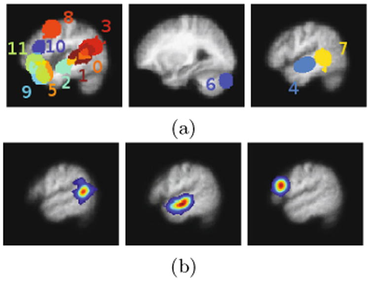
Estimated dictionary. (a) Three slices of a map showing the spatial support of the extracted dictionary elements. Different colors correspond to distinct dictionary elements where there is some overlap between dictionary elements. From left to right: left frontal lobe and temporal regions, right cerebellum, right temporal lobe. Dictionary element indices correspond to those in Fig. 2. (b) A single slice from three different estimated dictionary volumes. From left to right: left posterior temporal lobe, left anterior temporal lobe, left inferior frontal gyrus.

To validate the estimated deformations, we apply the deformation learned by the model to left-out time course data for each subject and perform the standard weighted random effects analysis. We then look at significance values within the support of each dictionary element. Importantly, for drawing conclusions on the group-level parcels defined by the estimated dictionary elements, within each parcel, it is the peak and regions around the peak that are of interest rather than the full support of the dictionary element. Thus, to quantify the advantage of our method, within each dictionary element, we compare the top 25% highest significance values for our method versus those of anatomical alignment (Fig. 2). We observe that accounting for functional variability via deformations results in substantially higher peak significance values within the estimated group-level parcels, suggesting better overlap of these functional activation regions across subjects. On average, our method improves the significance of group analysis by roughly 2 orders of magnitude when looking at the top 25% significance values.

Fig. 2.

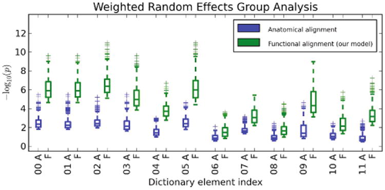
Box plots of top 25% weighted random effects analysis significance values within dictionary element supports. For each dictionary element, “A” refers to anatomical alignment, and “F” refers to alignment via deformations learned by our model.

Even if we look at the top 50% of significance values in each dictionary element, the results remain similar to those in Fig. 2.

4 Conclusions

We developed a model that accounts for spatial variability of functional regions in the brain via deformations of weighted dictionary elements. Learning model parameters and estimating deformations yields correspondences of functional units in the brain across subjects. We demonstrate our model in a language fMRI study, which contains substantial variability. We plan to validate the detected parcels using data from different fMRI language experiments.

References

- 1.Dempster AP, Laird NM, Rubin DB. Maximum likelihood from incomplete data via the EM algorithm. Journal of the Royal Statistical Society. 1977;39(1):1–38. [Google Scholar]
- 2.Depa M, Sabuncu MR, Holmvang G, Nezafat R, Schmidt EJ, Golland P. Robust Atlas-Based Segmentation of Highly Variable Anatomy: Left Atrium Segmentation. In: Camara O, Pop M, Rhode K, Sermesant M, Smith N, Young A, editors. STACOM-CESC 2010 LNCS. Vol. 6364. Springer; Heidelberg: 2010. pp. 85–94. [DOI] [PMC free article] [PubMed] [Google Scholar]
- 3.Fedorenko E, Hsieh PJ, Nieto-Castañón A, Whitfield-Gabrieli S, Kanwisher N. New method for fMRI investigations of language: Defining ROIs functionally in individual subjects. Neurophysiology. 2010;104:1177–1194. doi: 10.1152/jn.00032.2010. [DOI] [PMC free article] [PubMed] [Google Scholar]
- 4.Olshausen B, Field D. Emergence of simple-cell receptive field properties by learning a sparse code for natural images. Nature. 1996;381:607–609. doi: 10.1038/381607a0. [DOI] [PubMed] [Google Scholar]
- 5.Sabuncu MR, Singer BD, Conroy B, Bryan RE, Ramadge PJ, Haxby JV. Function-based intersubject alignment of human cortical anatomy. Cerebral Cortex. 2010;20(1):130–140. doi: 10.1093/cercor/bhp085. [DOI] [PMC free article] [PubMed] [Google Scholar]
- 6.Thirion B, Pinel P, Tucholka A, Roche A, Ciuciu P, Mangin JF, Poline JB. Structural analysis of fMRI data revisited: improving the sensitivity and reliability of fMRI group studies. IEEE Transactions in Medical Imaging. 2007;26(9):1256–1269. doi: 10.1109/TMI.2007.903226. [DOI] [PubMed] [Google Scholar]
- 7.Varoquaux G, Gramfort A, Pedregosa F, Michel V, Thirion B. Multi-subject Dictionary Learning to Segment an Atlas of Brain Spontaneous Activity. In: Székely G, Hahn HK, editors. IPMI 2011 LNCS. Vol. 6801. Springer; Heidelberg: 2011. pp. 562–573. [DOI] [PubMed] [Google Scholar]
- 8.Vercauteren T, Pennec X, Perchant A, Ayache N. Symmetric Log-Domain Diffeomorphic Registration: A Demons-Based Approach. In: Metaxas D, Axel L, Fichtinger G, Székely G, editors. MICCAI 2008, Part I LNCS. Vol. 5241. Springer; Heidelberg: 2008. pp. 754–761. [DOI] [PubMed] [Google Scholar]
- 9.Xu L, Johnson TD, Nichols TE, Nee DE. Modeling inter-subject variability in fMRI activation location: a bayesian hierarchical spatial model. Biometrics. 2009;65(4):1041–1051. doi: 10.1111/j.1541-0420.2008.01190.x. [DOI] [PMC free article] [PubMed] [Google Scholar]