Quantitative Interpretation of FRET Experiments via Molecular Simulation: Force Field and Validation

Abstract

Molecular simulation is a valuable and complementary tool that may assist with the interpretation of single-molecule Förster resonance energy transfer (FRET) experiments, if the energy function is of sufficiently high quality. Here we present force-field parameters for one of the most common pairs of chromophores used in experiments, AlexaFluor 488 and 594. From microsecond molecular-dynamics simulations, we are able to recover both experimentally determined equilibrium constants and association/dissociation rates of the chromophores with free tryptophan, as well as the decay of fluorescence anisotropy of a labeled protein. We find that it is particularly important to obtain a correct balance of solute-water interactions in the simulations in order to faithfully capture the experimental anisotropy decays, which provide a sensitive benchmark for fluorophore mobility. Lastly, by a combination of experiment and simulation, we address a potential complication in the interpretation of experiments on polyproline, used as a molecular ruler for FRET experiments, namely the potential association of one of the chromophores with the polyproline helix. Under conditions where simulations accurately capture the fluorescence anisotropy decay, we find at most a modest, transient population of conformations in which the chromophores associate with the polyproline. Explicit calculation of FRET transfer efficiencies for short polyprolines yields results in good agreement with experiment. These results illustrate the potential power of a combination of molecular simulation and experiment in quantifying biomolecular dynamics.

Introduction

Because of their ability to resolve distances and dynamics of subpopulations of molecules in a sample, single-molecule experiments are a powerful tool for dissecting the properties of biomolecules (1,2), properties that can usually only be indirectly inferred from ensemble experiments. Such experiments include single-molecule atomic force microscopy (3), optical tweezers (2), or Förster resonance energy transfer (FRET) experiments (1). However, the information about the macromolecule is typically limited, because usually only a single distance is measured; with ever-increasing accessible timescales (4–6), simulations can therefore fill the gap in modeling details, provided they can also reproduce the single-molecule results.

Single-molecule FRET, in particular, has been applied to a wide range of problems in which molecular simulations have proved to be a useful complement. Examples include the distributions of distances and dynamics within unfolded or disordered proteins (7–13), protein-folding dynamics (14), protein association (15), and even the calibration of FRET efficiencies using a polyproline molecular-ruler concept (16–18). One important consideration in such simulations is how to model the chromophores themselves. Explicit inclusion of the chromophores may have several advantages. For example, one may want to determine the potential influence of the chromophores on the experiment (19,20). Explicit chromophores also help to address directly some of the assumptions about chromophore dynamics that are generally invoked to facilitate interpretation of single-molecule experiments (16,17,21–24); and even in cases where these conditions are not completely satisfied, the simulation and experiments may potentially still be used in conjunction to obtain quantitative distance information from FRET data, provided that the energy function for the chromophores is trustworthy.

To date, a number of groups have proposed parameters for modeling chromophores in solution, in most cases with specific applications in mind (22,25–28). However, these parameters have, for the most part, not been quantitatively validated against experiment; part of the reason may be a lack of suitable experimental data, or that good agreement of dynamical properties is not expected due to the viscosity of commonly used water models such as TIP3P (29) being too low. In this article, we derive a set of parameters for a pair of chromophores frequently employed in single-molecule experiments on proteins (7,8,14,17,18,30–38), namely AlexaFluor 488 and AlexaFluor 594 (39) (henceforth Alexa 488 and Alexa 594) (Fig. 1), to be used in conjunction with the TIP4P/2005 water model (40). We test this set of parameters against several experimental observables that are particularly sensitive to dye-protein interactions: nanosecond fluorescence correlation functions for chromophore-tryptophan binding, fluorescence anisotropy decays for chromophores attached to a protein or to a polyproline peptide, and FRET efficiencies. We find that an empirical scaling of protein-water interactions, recently introduced to improve the treatment of protein-protein association, and of intrinsically disordered and unfolded proteins (41), markedly improves the results. Lastly, we address a concern regarding polyproline experiments raised by molecular simulations: namely that one or both of the chromophores may stick to the hydrophobic polyproline helix, thus complicating the experimental interpretation even further (17,18). We show that for force fields in which the anisotropy decay matches experiment, the population of chromophores bound to the polyproline is 20–50%, with average associated lifetimes of <10 ns.

Figure 1.

Molecules used for dye parameterization and testing: (A) AlexaFluor 488 free acid, (B) AlexaFluor 594 free acid, (C) poly-L-proline (shown is polyproline-11 labeled via an N-terminal Gly with Alexa594 and via a C-terminal Cys with Alexa488), (D) N-terminally labeled CspTm (via Cys at position 2, Alexa 488 shown), and (E) C-terminally labeled CspTm (via Cys at position 68, Alexa 488 shown). In (C), the vectors used for transition dipole moments are indicated on the donor and acceptor (r_D and r_A, respectively), together with the vectors parallel and perpendicular to the polyproline axis (r_|| and r_⊥, respectively). To see this figure in color, go online.

Materials and Methods

Parameterization of chromophores

Our priority in determining parameters was to obtain reasonable nonbonded interactions, as the most critical feature of the model is how the chromophores interact with other chromophores and with proteins. We use standard AMBER (University of California, San Francisco, San Francisco, CA; ambermd.org) atom types for all of the atoms in the two chromophores, thus fixing the Lennard-Jones parameters (note that these parameters are common to most all-atom AMBER force fields from ff94 onwards); angle and torsion terms were added by analogy with similar terms in the AMBER force field. Charges were determined using the restrained electrostatic potential (RESP) fitting as implemented in the ANTECHAMBER program (42,43). For consistency with AMBER charges (44), electrostatic potentials were determined with restricted Hartree-Fock, assuming all carboxylate groups to be deprotonated, i.e., net charge of −3 for each dye in its free form; the geometry of each molecule was first optimized with the same method. We used the 6-31+G^∗ basis set in place of the 6-31G^∗ normally used for deriving RESP charges, the diffuse basis functions being included due to the second-row atoms in these molecules. We also found that using this basis set gave more reasonable results in the geometry optimizations. As an alternative, we also obtained a set of RESP charges from an electrostatic potential computed using density functional theory with the B3LYP functional (45) and 6-311+G^∗ basis. Quantum chemistry calculations were all done with the GAUSSIAN 03 software package (46). All parameters not present in the standard AMBER ff03^∗/ff03w protein force field are given in Tables S1 and S2 in the Supporting Material. Atom-types and charge parameters for the aliphatic linker were also chosen to be similar to related groups in AMBER force fields. The new parameters are listed in the Supporting Material and are available from the authors in GROMACS format (www.gromacs.org) in conjunction with the AMBER ff03ws and the AMBER ff99SBws force fields.

Protein simulations

We conducted simulations with a number of combinations of protein force fields and water models. The water models were either the commonly used three-site model, TIP3P (29), or a more recently developed four-site model, TIP4P/2005 (40). For TIP3P, we always determine protein-water Lennard-Jones interactions based on standard Lorenz-Berthelot mixing rules. For TIP4P/2005, we considered in addition a second type of mixing rule in which we scale the protein-water and chromophore-water interactions by a factor λ_pw. Specifically, for each atom i in the protein or chromophore, we set ${\epsilon }_{Oj}={\lambda }_{pw}{\epsilon }_{Oj}^{LB}$, where ${\epsilon }_{Oj}^{LB}$ is the Lennard-Jones ε for interactions between water oxygen and atom j given by the Lorentz-Berthelot mixing rules and ε_Oj as the final scaled parameter. In the results, the original water name TIP4P/2005 implies standard Lorentz-Berthelot mixing rules (λ_pw = 1), while other models are specified using the notation TIP4P/2005(λ_pw). The model TIP4P/2005(1.10), i.e., λ_pw = 1.10, corresponds to the recently suggested scaling of protein-water interactions in AMBER force fields in order to improve the properties of intrinsically disordered proteins and protein-protein interactions (41). The protein force fields were all based on the AMBER ff03 (47) and AMBER ff99SB (48) energy functions. However, there were further modifications to the backbone torsion angles used, in order to obtain the correct helix propensity in each water model. These protein force fields are: AMBER ff03^∗ (for TIP3P water) (49), AMBER ff03w (for TIP4P/2005 water) (50), AMBER ff03ws (for TIP4P/2005(λ_pw) water, λ_pw ≠ 1) (41), and AMBER ff99SBws (for TIP4P/2005(λ_pw) water and λ_pw ≠ 1) (41), and have all been previously described. Any scaling of protein-water interactions was also applied to chromophore-water interactions. Note that for clarity and consistency, we explicitly list which water model is being used even when it is implied by the protein force field, but this should not be taken to suggest that other combinations could have been used.

Molecular-dynamics simulations were carried out with the GROMACS 4.x simulation package (51,52), at a constant temperature of 298 K using a stochastic velocity rescaling thermostat (53) with a coupling time of 1 ps and pressure of 1 bar with a Parrinello-Rahman barostat (54) and a coupling time of 5 ps. Simulations were run for 0.3–1 μs for each system studied (the length of each simulation is given in Table S5), using a 2-fs time step. All bond lengths were constrained to their equilibrium values from the parameter set using the LINCS algorithm (55). Nonbonded parameters were similar to those used in previous work (41). That is, Coulomb energy and forces were calculated by the particle-mesh Ewald method (56) with a 0.9-nm real-space cutoff and 0.12-nm-grid spacing. Lennard-Jones parameters were treated with a twin-range method in which forces for atom pairs closer than 0.9 nm were updated at every time step and those for pairs between 0.9 and 1.4 nm were updated every 10 steps. Mean-field corrections to the energy and pressure for atom pairs beyond 1.4 nm were included.

Calculation of fluorescence anisotropy

The decay in fluorescence anisotropy in the simulated systems was evaluated from the decay of the correlation function (57)

$$r\left(t\right)=r_0\langle P_2\left(\hat{\mu }\left(t\right)\cdot \hat{\mu }\left(0\right)\right)\rangle ,$$ (1)

where P₂(x) = (3x² − 1)/2 is the second-order Legendre polynomial, and $\hat{\mu }\left(t\right)$ is the unit vector in the direction of the transition dipole moment of the respective fluorophore at time t. The coefficient r₀ corresponds to the fundamental anisotropy of 2/5 if the excitation and emission dipole moments are colinear. Here we use for r₀ a value of 0.38, the limiting anisotropy of Alexa 488 and 594 determined experimentally (58). For the cold-shock protein CspTm, a reference correlation function representing the rotational motion of the protein only was constructed by averaging the P₂ correlation functions for five vectors within the protein (between backbone atoms in secondary structure), specifically between the Cα atoms of residues 17 and 48, 15 and 58, 15 and 46, 58 and 65, and 8 and 27.

Calculating transfer rates from protein-dye simulations

We use Förster theory (59,60) to calculate the transfer rates between the chromophores. The transfer rate k_ET(x) for configuration x (corresponding to a frame of the simulation trajectory) is given by

$$k_{ET}\left(x\right)=\frac{3}{2}{k}_D{R}_0^6\frac{{\kappa }^2\left(x\right)}{R^6\left(x\right)},$$ (2)

where k_D is the donor fluorescence decay rate in the absence of an acceptor; R₀ is the Förster radius for κ² = 2/3, determined spectroscopically for Alexa488 and Alexa594 to be ∼5.4 nm (30,61); R is the separation between the chromophores; and the orientational factor κ is given by

$$\kappa ={\hat{\mu }}_D\cdot {\hat{\mu }}_A-3\left(\hat{R}\cdot {\hat{\mu }}_A\right)\left(\hat{R}\cdot {\hat{\mu }}_D\right),$$ (3)

where ${\hat{\mu }}_D$ and ${\hat{\mu }}_A$ are unit vectors in the direction of the donor and acceptor transition dipoles respectively; and $\hat{R}$ is a unit vector pointing between donor and acceptor. We assume that the donor and acceptor transition dipole moments are approximately aligned with the long axis of each chromophore system (defined by the vectors between atoms C11 and C12 within each chromophore; see Fig. S1 in the Supporting Material), and the distance between the chromophores is taken to be that between the C1 atoms of each chromophore. The decay in donor fluorescence intensity is evaluated by calculating the survival probability of the excited state with a fluctuating transfer rate, averaged over all possible time origins along a simulation trajectory:

$$I\left(t\right)=\langle \text{exp}\left(-{\int }_0^t\left[k_D+k_{ET}\left(\tau \right)\right]d\tau \right)\rangle .$$ (4)

The average FRET efficiency was obtained by integration of the intensity decay (or lifetime distribution),

$$\langle E\rangle =1-k_D\underset{0}{\overset{t_{\text{max}}}{\int }}I\left(t\right)dt,$$ (5)

where the maximum integration time t_max was chosen as 20 ns, by which time the fluorescence had essentially decayed to zero.

Time-resolved fluorescence anisotropy measurements

Fluorescently labeled samples of the cold-shock protein from Thermotoga maritima were prepared essentially as described previously in Schuler et al. (30) and Soranno et al. (62), but only a single donor or a single acceptor dye was attached via maleimide chemistry to one of the two Cys residues in the protein (positions 2 and 68) to avoid complications from the FRET process for interpreting the anisotropy results. (Pro)₁₀-Cys-Alexa488 was also prepared as described previously in Schuler et al. (33) by reacting Alexa 488 maleimide with the Cys residue in the peptide and purification by reversed-phase HPLC. Ensemble measurements were performed in 50 mM sodium phosphate buffer, pH 7.0 at 22°C with protein or peptide concentrations of ∼1 μM. For time-resolved anisotropy measurements, donor or acceptor were excited with picosecond pulses at a wavelength range selected by a HQ 470/40 band-pass filter for donor excitation and by a z582/15 band-pass filter for acceptor excitation (Chroma Technology, Bellows Falls, VT) and a pulse frequency of 20 MHz (Optical Supercontinuum Systems SC450-4, 20 MHz; Fianium, Southampton, UK). Fluorescence emission was filtered with an ET 525/50 filter (Chroma Technology) for donor emission and a HQ 650/100 filter (Chroma Technology) for acceptor emission. The signal was detected with a microchannel plate photomultiplier tube (R3809U-50; Hamamatsu, Hamamatsu City, Japan), preamplified (PAM 102-M; PicoQuant Photonics North America, West Springfield, MA), and recorded by a PicoHarp 300 photon-counting module (PicoQuant Photonics North America), resulting in a width of the instrument response function of ∼80 ps, as described previously in Nettels et al. (63). The G-factor was determined from

$$G=\frac{I_{HV}}{I_{HH}},$$ (6)

where I_HV is the intensity of the vertically polarized fluorescence emission component after excitation with horizontally polarized light, and I_HH is the horizontally polarized emission component after excitation with horizontally polarized light. The anisotropy decay, r(t), was calculated from the decay of I_VV(t) and I_VH(t) according to

$$r\left(t\right)=\frac{I_{VV}-G{I}_{VH}}{I_{VV}+2G{I}_{VH}}.$$ (7)

The instrument response function was determined using scattered excitation light with a dilute Ludox (Sigma-Aldrich, St. Louis, MO) solution.

Results

Chromophore-tryptophan association

Accurate force-field parameters are clearly a prerequisite for using simulations to interpret single-molecule FRET experiments. Therefore, we first validate the parameters we have obtained for Alexa488 and Alexa594, two of the fluorophores that are most commonly used in single-molecule experiments (7,8,14,17,18,30–38). An interaction of the fluorophores that can complicate the interpretation of single-molecule FRET experiments is their transient binding to exposed aromatic amino-acid side chains, especially to the indole ring of tryptophan, which leads to static quenching (37,64). We thus chose as a first test-data set the kinetics of association of each chromophore (without any linker attached, Fig. 1, A and B) with zwitterionic tryptophan free in solution. Quenching of the fluorescence of Alexa 488 and 594 by tryptophan association has allowed the association and dissociation rates to be determined from nanosecond fluorescence correlation spectroscopy (37). Here we have run long simulations of one copy of the chromophore and one Trp molecule in explicit TIP4P/2005 water at a concentration of ∼29 mM each. In Fig. 2, A and B, we show the number of contacts between Trp and Alexa488 and Alexa 594, respectively, as a function of time (the number of contacts is taken as the number of atom pairs within 0.6 nm). We obtain an approximately two-state picture of association/dissociation in each case, with the molecules being mostly bound. Note that the bound states are somewhat heterogeneous, but almost all involve a stacking of the aromatic ring systems of the two molecules. Some representative structures for this associated state are shown in Fig. 2, E and F. We quantify the binding kinetics and equilibria by defining the unbound state as having <0.1 contacts and bound as >400 contacts, and determining the rates from the average binding or unbinding times (Table 1). For Alexa488, using the RESP (42) partial charges determined from the HF/6-31+G^∗ electrostatic potential, we obtain a fair agreement with both association rates and equilibrium constants; however, for Alexa 594, this charge set results in an affinity roughly an order of magnitude higher than experiment.

Figure 2.

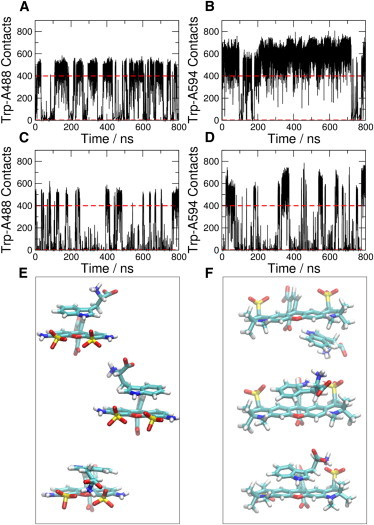
Simulations of fluorophore-tryptophan interactions. (A–D) Contact formation between dyes and tryptophan at ∼29 mM. (A) Alexa488, TIP4P/2005; (B) Alexa594, TIP4P/2005; (C) Alexa488, TIP4P/2005(1.10); and (D) Alexa594, TIP4P/2005(1.10). (Broken lines) Cutoffs for making (>400 contacts) and breaking (<0.1 contacts) a dye-Trp interaction. (E and F) Representative examples of Alexa488:Trp and Alexa594:Trp complexes formed upon association, respectively. To see this figure in color, go online.

Table 1.

Kinetic and equilibrium parameters for chromophore-tryptophan association

Chromophore	kon/M−1 ns−1	koff/ns−1		Kd/mM
Alexa488, experimenta	1.2 (0.2)		0.071 (0.014)	59 (17)
Alexa488 qHF, TIP4P/2005	2.7 (0.5)		0.052 (0.012)	20 (6)
Alexa488 qHF, TIP4P/2005(1.10)	1.4 (0.3)		0.128 (0.036)	91 (32)
Alexa488 qHF, TIP3P	14.3 (2.6)		0.102 (0.019)	7.1 (1.8)
Alexa488 qDFT, TIP4P/2005	3.2 (0.9)		0.075 (0.021)	23 (9)
Alexa488 qDFT, TIP4P/2005(1.10)	1.8 (0.5)		0.134 (0.042)	75 (30)
Alexa594, experiment	1.1 (0.2)		0.036 (0.007)	33 (9)
Alexa594 qHF, TIP4P/2005	3.1 (0.7)		0.012 (0.008)	3.9 (2.7)
Alexa594 qHF, TIP4P/2005(1.10)	1.3 (0.3)		0.083 (0.020)	63 (20)
Alexa594 qHF, TIP3P	11.9 (3.3)		0.037 (0.011)	3.1 (1.3)
Alexa594 qDFT, TIP4P/2005	5.2 (1.0)		0.006 (0.003)	1.2 (0.6)
Alexa594 qDFT, TIP4P/2005(1.10)	1.8 (0.2)		0.139 (0.059)	76 (34)

The chromophores have charges determined from a Hartree-Fock electrostatic potential (q_HF) or DFT electrostatic potential (q_DFT), and are used together with the TIP3P, TIP4P/2005, or TIP4P/2005(1.10) water models (the last is TIP4P/2005 with solute-water interactions scaled by a factor λ_pw = 1.10). The tryptophan concentration was 29 mM in simulations and 40 mM in experiment (37).

^aExperimental data taken from Haenni et al. (37). Experimental errors are estimated as 20% of the reported rates. Note that these data were recorded for each dye together with C₅ maleimide linker, reacted with β-mercaptoethanol. However, essentially identical results, considering experimental error, are obtained for the free dyes.

The excess affinity of Alexa594 and Trp may be related to the poor solvation of proteins in water for these force fields, which has recently been noted (41,65–68). The long-term solution to that problem is likely to be a refitting of the protein Lennard-Jones parameters, which our chromophore model shares with the protein force field (68,69). However, it has been determined that an approximate correction can be made by globally scaling the Lennard-Jones well depth for protein-water interactions, resulting in much improved results for protein binding affinities as well as dimensions for unfolded states (41). We therefore applied the same correction to the chromophore-water interactions; we note that this is also the most straightforward approach to adopt when the chromophore is covalently attached to the protein. The results with this protein-water scaling (TIP4P/2005(1.10) water model, Fig. 2, C and D; Table 1) have a relatively small effect on the association/dissociation rates and equilibrium for Trp and Alexa488, but for Trp and Alexa594 they result in an affinity much closer to experiment, suggesting that the modified protein-solvent interactions are not detrimental and represent an improvement.

For comparison, we have also considered RESP charges obtained from an electrostatic potential calculated from density functional theory. The results (Table 1) are very similar to those obtained with the Hartree-Fock electrostatic potential usually used with RESP, and so we continue with the Hartree-Fock-derived charge set. We have also considered using TIP3P as an alternative solvent model. Although this model has a viscosity ∼3 times lower than water, which complicates a quantitative comparison with experiment, it is still the most commonly used water model in biomolecular simulations. We find in this case that the affinity of the dyes for tryptophan is approximately an order of magnitude too strong, a problem that is most likely related to the imbalance of protein-water interactions because the dyes share their Lennard-Jones parameters with the protein force field (41). Most of the difference is in the on-rate. The small change in the off-rate is likely due to the opposing effects of tighter binding and lower solvent viscosity. The on-rate is increased by a factor slightly greater than reduction in solvent viscosity, most likely because a larger fraction of collisions are likely to lead to productive binding, due to the weaker competing interactions with water.

Protein-chromophore conjugates

As a second test of the chromophore parameters, which is sensitive also to chromophore-protein interactions, we used time-resolved fluorescence anisotropy data for each chromophore attached to the cold-shock protein CspTm, a system that has been investigated in great detail in single-molecule FRET experiments (8,9,30,61,62,70–72), in a single-labeled configuration. These correlation functions measure the time over which the chromophore loses correlation with its original orientation, which is due to a combination of slow overall protein tumbling, as well as a faster reorientation of the chromophore with respect to the protein. The protein contains a cysteine residue at both the N- and C-termini, one of which is (nonspecifically) labeled with either Alexa488 or Alexa594. The anisotropy decay has been measured experimentally using polarization-selective time-correlated single-photon counting (see Materials and Methods). From simulation, we have computed the P₂ correlation function r(t) for a vector representing the fluorophore transition dipole moment for the labeled proteins, globally scaled to match the empirically determined limiting anisotropy r₀ ∼ 0.38 (58). We initially performed simulations with AMBER ff03w, and the TIP4P/2005 water model for which it is optimized. Because the experiment is performed on a mixture of two populations—one labeled at the C-terminus and the other at the N-terminus—we have carried out simulations for each of these scenarios (Fig. 3). In each case, we find that the protein remains stable over the course of the simulation, with slightly larger fluctuations of the loops with AMBER ff03ws and TIP4P/2005(1.10) (Fig. S2). Both labeling schemes result in similar anisotropy decays, which are also in good agreement with the experimental curves. We have characterized the dynamics by fitting biexponential functions to both simulated and experimental decays, finding a slow phase for molecular tumbling of 3–5 ns and a faster phase of 0.1–0.5 ns arising from chromophore reorientation within a static molecular reference frame (Table 2). The amplitude of the fast phase is larger for the Alexa594 conjugates. However, with this force-field combination, the anisotropy decay is still slightly too slow. The agreement with experiment is improved by using TIP4P/2005(1.10) water (with scaled protein-water interactions) and the corresponding AMBER ff03ws protein force field, suggesting that interaction of the dyes with the protein with AMBER ff03w and TIP4P/2005 is slightly too strong, resulting in transient sticking to the protein surface. The anisotropy for such a population would decay as for a vector orientation fixed relative to the protein; an example of such a decay is shown by broken curves in each case in Fig. 3, based on intramolecular protein vectors between backbone atoms in regions of secondary structure, which fluctuate only slightly as a result of internal protein motions.

Figure 3.

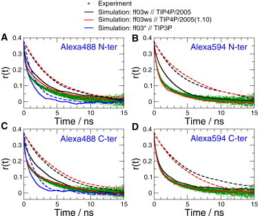
Fluorescence anisotropy decay for chromophores attached to CspTm. (A) AlexaFluor 488, N-terminal label; (B) AlexaFluor 594, N-terminal label; (C) AlexaFluor 488, C-terminal label; and (D) AlexaFluor 594, C-terminal label. (Green points) Experimental data; (solid black curve) anisotropy decays from simulations with TIP4P/2005; (solid red curve) anisotropy decays from simulations with TIP4P/2005(1.10); (solid blue curve) anisotropy decays from simulations with TIP3P, respectively; and (broken lines with corresponding colors) molecular correlation function of the protein $\langle P_2\left(\hat{\mu }\left(t\right)\cdot \hat{\mu }\left(0\right)\right)\rangle$ for fixed intramolecular unit vectors $\hat{\mu }$. The molecular correlation function has been scaled by 0.38 to fit on the same scale as the experimentally determined anisotropy decay. To see this figure in color, go online.

Table 2.

Fit parameters for anisotropy decay of protein-dye conjugates

System	τmol/ns	τfast/ns	Amol
Alexa488, experiment	3.80 (0.02)	0.24 (0.01)	0.52 (0.002)
Alexa488, ff03∗//TIP3P, N-terminal	1.31 (0.13)	0.06 (0.06)	0.78 (0.07)
Alexa488, ff03w//TIP4P/2005, N-terminal	5.03 (0.72)	0.47 (0.16)	0.59 (0.09)
Alexa488, ff03w//TIP4P/2005, C-terminal	3.48 (0.31)	0.11 (0.04)	0.81 (0.03)
Alexa488, ff03ws//TIP4P/2005(1.10), N-terminal	5.19 (1.73)	0.34 (0.21)	0.51 (0.10)
Alexa488, ff03ws//TIP4P/2005(1.10), C-terminal	3.70 (0.52)	0.18 (0.02)	0.56 (0.05)
Alexa594, experiment	3.55 (0.03)	0.46 (0.01)	0.43 (0.004)
Alexa594, ff03∗//TIP3P, N-terminal	1.57 (0.86)	0.34 (0.16)	0.57 (0.09)
Alexa594, ff03w//TIP4P/2005, N-terminal	3.29 (1.58)	0.47 (0.51)	0.73 (0.09)
Alexa594, ff03w//TIP4P/2005, C-terminal	7.79 (2.54)	0.76 (0.11)	0.29 (0.08)
Alexa594, ff03ws//TIP4P/2005(1.10), N-terminal	2.64 (0.26)	0.43 (0.05)	0.46 (0.06)
Alexa594, ff03ws//TIP4P/2005(1.10), C-terminal	3.65 (1.03)	0.50 (0.05)	0.41 (0.07)

Data were fit to the function $r\left(t\right)=r_0\left(\left(1-A_{\text{mol}}\right)e^{-t/{\tau }_{\text{fast}}}+A_{\text{mol}}\right)e^{-t/{\tau }_{\text{mol}}}$, where r₀ ≡ 0.38. The notation after the chromophore name is protein force-field//water model. Experimental data are for CspTm nonspecifically labeled with a single chromophore at either the N- or C-terminal labeling site. Note that in each simulation, the protein force field used was optimized to be used with the water model specified. We only list the water models explicitly for clarity. Errors for experiment are estimated by Monte Carlo resampling of the original data, while for simulation, errors were estimated from separate fits after dividing the data into 10 equal blocks.

Together, the results suggest that with the chromophore parameters presented, and scaled protein-water interactions, we obtain a good description of both the magnitude of interactions between dyes and the protein, as well as of the diffusive dynamics of the conjugated chromophore. Lastly, we have also calculated the anisotropy decay for the N-terminally attached chromophores using the AMBER ff03^∗ force field and TIP3P water, the most frequently used water model in biomolecular simulations. The relaxation in that case is too fast, as a consequence of the viscosity of this model being ∼3 times lower than that of water.

Polyproline-chromophore dynamics

Oligoproline molecules have a long history of use as molecular rulers in order to test Förster’s theory for resonance energy transfer (17,18,33,73,74). However, like any real molecular system, there are potential complications in the interpretation of the experiment, one of which is a small population (∼2%) of residues that adopt a cis-proline conformation (18). Another potential complication, which has been suggested based on molecular simulations, is the interaction of one or both of the dyes with the polyproline helix (17,18). In particular, a stable interaction of the C-terminal Alexa488 chromophore has been suggested for polyprolines in the series Alexa594-Gly-(Pro)_n-Cys-Alexa488, in which Alexa594 is linked to the N-terminal amine and Alexa488 to the sulfhydryl group of the C-terminal cysteine (17). In order to address this potential problem and further test the force field, we have investigated a series of polyproline-dye conjugates. We first study the C-terminal label in the context of the construct (Pro)₁₀-Cys-Alexa488. Microsecond molecular-dynamics simulations of this system using the AMBER ff03w protein force field and TIP4P/2005 water indeed show pronounced transient sticking of the Alexa488 to the polyproline. This was assessed by the minimum distance between any two atoms of the prolines and the chromophore (Fig. 4 E), resulting in an anisotropy decay that is significantly too slow relative to experiment (Fig. 4 A). Because this may be due to too strong dye-protein interactions as above, we ran a series of simulations with scaled interactions λ_pw between solute and solvent of 1.10, 1.15, and 1.20 (Fig. 4, B–D, respectively), in which the water models are referred to as TIP4P/2005(1.10), TIP4P/2005(1.15), and TIP4P/2005(1.20). We find that TIP4P/2005(1.10) hardly changes the result, while TIP4P/2005(1.15) and TIP4P/2005(1.20) result in much improved agreement with experiment—and also reduced sticking of the dye to the peptide (the root-mean-square deviation of the anisotropy decay from experiment, and fraction bound, are shown in Fig. 5).

Figure 4.

Quantifying transient contact formation between Alexa 488 and polyproline in the molecule (Pro)₁₀-Cys-Alexa488. (A–D) Decay of experimental fluorescence anisotropy (black), decay of anisotropy in simulations for Alexa 488 using the AMBER ff03w force field for polyproline (red), for a vector parallel to the polyproline axis (dot-dash black line), and for a vector perpendicular to the polyproline axis (dashed black line). (Blue curves) Decays of Alexa 488 anisotropy when the AMBER ff99SBw force field is used for polyproline. Solute-water interactions are scaled by the factors λ_pw indicated in each panel. (E–H) Trajectories of minimum Alexa488-Proline distance corresponding to the anisotropy decays in the panels to the left, for the AMBER 03 protein force field. (Broken red lines, E–H) Thresholds of 0.25 and 1.0 nm used to define bound and unbound configurations. To see this figure in color, go online.

Figure 5.

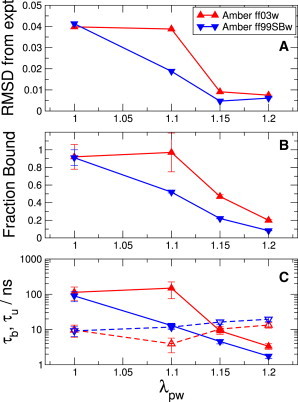
Dependence of the association of Alexa488 with proline residues in (Pro)₁₀-Cys-Alexa488 on the solute-water interaction scaling factor, λ_pw, for AMBER ff03w and AMBER ff99SBw. (A) Root-mean-square difference between experimental and simulation anisotropy data, (B) fraction of time Alexa488 is associated with proline residues, and (C) binding (open symbols, broken lines) and unbinding (solid symbols, solid lines) times as a function of λ_pw.

Although it is somewhat disappointing that the TIP4P/2005(1.10) model previously determined to be optimal for protein-water interactions (41) is not sufficient to obtain agreement with experiment here, it may not be entirely surprising, given the substantial remaining errors in solvation free energies of specific residues. Unlike heteropolymeric protein sequences, the simple proline repeat will tend to amplify any shortcomings of the force field for that particular residue. Indeed, although the TIP4P/2005(1.10) model resulted in improved average solvation free energies for all residue side-chain analogs in AMBER ff03ws relative to TIP4P/2005, there was still a large root-mean-square difference (6.12 kJ mol⁻¹) (41) from experiment for the solvation free energies of side-chain analogs of specific residues (41,68). (Unfortunately, there is no clear definition of a side-chain analog for proline itself.) This reasoning is supported by results obtained for the (Pro)₁₀-Cys-Alexa488 conjugate with a different protein force field, AMBER ff99SBws, where the same TIP4P/2005(1.10) model was also found to be optimal for protein-water interactions (41). In this case, TIP4P/2005(1.10) already results in a fairer agreement of the anisotropy decay for the (Pro)₁₀-Cys-Alexa488 (Fig. 4 B). Taken together, these results justify our approach of considering polyproline as a special case. Naturally occurring heteropolymeric protein sequences would be less susceptible to this type of error accumulation, and the global scaling of 1.10 should still be used. For example, this global scaling appears to still be optimal for describing the binding of the chromophores to tryptophan, because using a larger scaling factor results in binding that is too weak (Table S6). Ultimately, a residue-specific or atom-specific correction to protein-water interactions should obviate the need for special treatment of homopolymeric sequences (68).

By comparing either the data for AMBER ff03w with TIP4P/2005(1.15) or AMBER ff99SBws with TIP4P/2005(1.10), we can determine the fraction of time where the dye is associated with the polyproline (defined as a minimum distance of <0.3 nm), yielding bound populations of 0.47 (0.02) and 0.52 (0.01). Increasing the protein-water interaction scaling factors by using TIP4P/2005(1.20) and TIP4P/2005(1.15) for the AMBER ff03w and AMBER ff99SBw force fields, respectively, results in a further slight improvement of the agreement with experiment (Fig. 5 A), and a decrease of the bound fraction to 0.20 (0.01) and 0.22 (0.01) respectively. By contrast, AMBER ff03w and AMBER ff99SBw with TIP4P/2005 result in bound fractions of 0.92 (0.14) and 0.91 (0.09), respectively. More dramatically, the time for unbinding of the dye-proline complex decreases from >100 ns with TIP4P/2005 to ≤10 ns with the optimal scaling (Fig. 5 C). In summary, it appears that the anisotropy data are compatible with a bound population in the range 0.2–0.5. The data may also be compatible with even lower bound fractions of <0.1, based on the results for AMBER ff99SBw with TIP4P/2005(1.20).

As a last comparison with experiment, we have analyzed FRET in polyproline-11 labeled with both donor and acceptor chromophores: Alexa594-Gly-(Pro)₁₁-Cys-Alexa488. Single-molecule experiments on freely diffusing molecules yield an average FRET efficiency of ∼0.87 (Fig. 6 A), in good agreement with earlier results (33). We have also determined the ensemble-averaged decay of donor fluorescence intensity from the simulations (Fig. 6 B). For the two force-field combinations that yield good agreement with the anisotropy data above (AMBER ff03w with TIP4P/2005(1.15) and AMBER ff99SBw with TIP4P/2005(1.10), the FRET efficiency calculated by integrating these decays is 0.83 (0.01) in both cases, while the efficiency for AMBER ff03w with TIP4P/2005 is 0.94 (0.01). The population of molecules containing at least one cis-proline is expected to be only ∼20% for Pro₁₁ (18), which may tend to increase the efficiency in experiment slightly, as we consider only all-trans polyproline in our simulations (an upper bound of ∼0.86 can be estimated by assuming that each of the 20% cis-containing prolines have a transfer efficiency of 1.0, and the remainder all-trans have the simulated efficiency of 0.83, given that exchange of populations is very slow).

Figure 6.

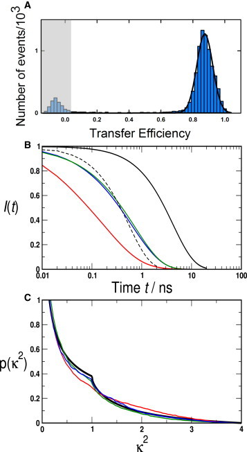
FRET for polyproline 11 with attached donor and acceptor chromophores. (A) Experimental transfer efficiency histogram for freely diffusing polyproline molecules, yielding a mean transfer efficiency of 0.87. The peak at E ≈ 0 (shaded area) is due to molecules lacking an active acceptor dye. (B) Donor fluorescence lifetime decays: (solid and broken black curves, respectively) exponential decays representing a donor lifetime of 4.2 ns (no acceptor) and of 0.55 ns (representing the experimental mean FRET transfer efficiency of 0.87 determined ratiometrically). (Red) AMBER ff03w with TIP4P/2005, (green) AMBER ff03w with TIP4P/2005(1.15), and (blue) AMBER ff99SBw with TIP4P/2005(1.10). (C) Distributions p(κ²) of the FRET orientational factor κ²: (black) expected p(κ²) for isotropically reorienting dye molecules. Simulation data are given with the same color code as in (B). To see this figure in color, go online.

We have also analyzed the distribution of the FRET orientational factor, κ², which is usually assumed to be isotropically averaged to a value of ∼2/3 when interpreting experimental results on samples showing low fluorescence anisotropy. A deviation of κ² from this ideal value has previously been attributed to association of chromophores with the polyproline helix (17). We find that the simulations with the scaled protein-water interactions have κ² distributions much closer to those expected for an isotropic distribution of chromophore orientations than for the original AMBER ff03w (Fig. 6 C). Values of κ² for these simulations are 0.72 (0.08) for AMBER ff03w with unscaled protein-water, 0.58 (0.05) for AMBER ff03w with λ_pw = 1.15 and 0.65 (0.03) for AMBER ff99SBw with λ_pw = 1.10.

We conclude our discussion by emphasizing that although we have treated the protein-water scaling as an adjustable parameter in our polyproline simulations due to the unusual sequence, we would not recommend that in most situations. The global scaling of λ_pw = 1.10 previously determined for use with AMBER ff03ws and AMBER ff99SBws should be sufficiently accurate for most heterogeneous protein sequences.

Conclusions

We have presented new force-field parameters for the Alexa488 and Alexa594 chromophores, which are among the most frequently used in single-molecule FRET experiments due to their high extinction coefficients and quantum yields and their good solubility in aqueous solutions. The new parameters are derived according to a standard AMBER RESP parameterization procedure (44), and are therefore compatible with the standard AMBER force fields—in particular, we have focused here on force fields derived from AMBER ff03 (47) and AMBER ff99SB (48). We obtain a good match with experimental fluorescence anisotropy decays, which are very sensitive tests of the dynamics of protein-dye conjugates, provided we use the TIP4P/2005 water model, and we scale the Lennard-Jones interactions between the protein and solvent. The TIP4P/2005 water model yields much better results for chromophore dynamics (e.g., anisotropy decay) than the commonly used TIP3P model, as expected from its more accurate viscosity.

Although the scaling of protein-solvent interactions is an empirical correction previously proposed to better capture protein-protein affinities (41,68), the scaled TIP4P/2005 water model also results in much better agreement with experiment for systems including the chromophores, again suggesting that a refitting of Lennard-Jones parameters in these force fields is needed in the long term. We then use molecular simulation to investigate the extent of association of chromophores with the polyproline helix in polyproline-dye conjugates. We do find a modest population of chromophores in contact with the proline residues, with ∼20–50% of the total being consistent with the available anisotropy and FRET data, but we cannot exclude the possibility of a lower population than this. Our results illustrate that a careful optimization of force-field parameters is essential for aiding the quantitative interpretation of single-molecule FRET experiments by molecular-dynamics simulations. In the absence of such optimization, as exemplified here by the established force fields without rescaling of water interactions, an overestimate of fluorophore-protein attraction can lead to a misinterpretation of the experimental results. An alternative approach is to ignore nonrepulsive interactions between dye and proteins and treat the fluorophores as freely diffusing within their sterically accessible volume (75,76), which can provide a reasonable approximation in favorable cases but may lead to an overestimate of dye mobility and can thus also bias the interpretation of the experimental result. Using a full atomistic simulation approach, as done here, incorporates the excluded volume effects of these other methods, but can also model favorable chromophore-protein interactions where they occur. The potential benefit of using MD simulations as opposed to diffusion within the accessible volume will naturally be system-dependent, and the relative merits of each in different situations will have to be assessed by systematic future studies.

In conclusion, we believe that the new chromophore parameters, in conjunction with an accurate water model and with modified protein-water interactions, can capture quite well the dynamics of these AlexaFluor chromophores when attached to proteins and peptides. This parameter set is thus expected to further improve the utility of molecular simulations for the structural and dynamic interpretation of single-molecule fluorescence experiments.

Author Contributions

R.B.B. and B.S. designed research; R.B.B., H.H., D.N., and B.S. performed research; R.B.B., H.H., D.N., and B.S. analyzed data; and R.B.B. and B.S. wrote the article.

References

- 1.Schuler B., Hofmann H. Single-molecule spectroscopy of protein folding dynamics—expanding scope and timescales. Curr. Opin. Struct. Biol. 2013;23:36–47. doi: 10.1016/j.sbi.2012.10.008. [DOI] [PubMed] [Google Scholar]
- 2.Greenleaf W.J., Woodside M.T., Block S.M. High-resolution, single-molecule measurements of biomolecular motion. Annu. Rev. Biophys. Biomol. Struct. 2007;36:171–190. doi: 10.1146/annurev.biophys.36.101106.101451. [DOI] [PMC free article] [PubMed] [Google Scholar]
- 3.Javadi Y., Fernandez J.M., Perez-Jimenez R. Protein folding under mechanical forces: a physiological view. Physiology (Bethesda) 2013;28:9–17. doi: 10.1152/physiol.00017.2012. [DOI] [PubMed] [Google Scholar]
- 4.Lindorff-Larsen K., Piana S., Shaw D.E. How fast-folding proteins fold. Science. 2011;334:517–520. doi: 10.1126/science.1208351. [DOI] [PubMed] [Google Scholar]
- 5.Piana S., Lindorff-Larsen K., Shaw D.E. Atomic-level description of ubiquitin folding. Proc. Natl. Acad. Sci. USA. 2013;110:5915–5920. doi: 10.1073/pnas.1218321110. [DOI] [PMC free article] [PubMed] [Google Scholar]
- 6.Bowman G.R., Voelz V.A., Pande V.S. Atomistic folding simulations of the five-helix bundle protein λ(6−85) J. Am. Chem. Soc. 2011;133:664–667. doi: 10.1021/ja106936n. [DOI] [PMC free article] [PubMed] [Google Scholar]
- 7.Müller-Späth S., Soranno A., Schuler B. Charge interactions can dominate the dimensions of intrinsically disordered proteins. Proc. Natl. Acad. Sci. USA. 2010;107:14609–14614. doi: 10.1073/pnas.1001743107. [DOI] [PMC free article] [PubMed] [Google Scholar]
- 8.Nettels D., Müller-Späth S., Schuler B. Single-molecule spectroscopy of the temperature-induced collapse of unfolded proteins. Proc. Natl. Acad. Sci. USA. 2009;106:20740–20745. doi: 10.1073/pnas.0900622106. [DOI] [PMC free article] [PubMed] [Google Scholar]
- 9.Wuttke R., Hofmann H., Schuler B. Temperature-dependent solvation modulates the dimensions of disordered proteins. Proc. Natl. Acad. Sci. USA. 2014;111:5213–5218. doi: 10.1073/pnas.1313006111. [DOI] [PMC free article] [PubMed] [Google Scholar]
- 10.Gnanakaran S., Hochstrasser R.M., García A.E. Nature of structural inhomogeneities on folding a helix and their influence on spectral measurements. Proc. Natl. Acad. Sci. USA. 2004;101:9229–9234. doi: 10.1073/pnas.0402933101. [DOI] [PMC free article] [PubMed] [Google Scholar]
- 11.Potoyan D.A., Papoian G.A. Regulation of the H4 tail binding and folding landscapes via Lys-16 acetylation. Proc. Natl. Acad. Sci. USA. 2012;109:17857–17862. doi: 10.1073/pnas.1201805109. [DOI] [PMC free article] [PubMed] [Google Scholar]
- 12.Echeverria I., Makarov D.E., Papoian G.A. Concerted dihedral rotations give rise to internal friction in unfolded proteins. J. Am. Chem. Soc. 2014;136:8708–8713. doi: 10.1021/ja503069k. [DOI] [PubMed] [Google Scholar]
- 13.Sherman E., Haran G. Coil-globule transition in the denatured state of a small protein. Proc. Natl. Acad. Sci. USA. 2006;103:11539–11543. doi: 10.1073/pnas.0601395103. [DOI] [PMC free article] [PubMed] [Google Scholar]
- 14.Rhoades E., Cohen M., Haran G. Two-state folding observed in individual protein molecules. J. Am. Chem. Soc. 2004;126:14686–14687. doi: 10.1021/ja046209k. [DOI] [PubMed] [Google Scholar]
- 15.Gambin Y., Deniz A.A. Multicolor single-molecule FRET to explore protein folding and binding. Mol. Biosyst. 2010;6:1540–1547. doi: 10.1039/c003024d. [DOI] [PMC free article] [PubMed] [Google Scholar]
- 16.Hoefling M., Grubmüller H. In silico FRET from simulated dye dynamics. Comput. Phys. Commun. 2013;184:841–852. [Google Scholar]
- 17.Hoefling M., Lima N., Grubmüller H. Structural heterogeneity and quantitative FRET efficiency distributions of polyprolines through a hybrid atomistic simulation and Monte Carlo approach. PLoS ONE. 2011;6:e19791. doi: 10.1371/journal.pone.0019791. [DOI] [PMC free article] [PubMed] [Google Scholar]
- 18.Best R.B., Merchant K.A., Eaton W.A. Effect of flexibility and cis residues in single-molecule FRET studies of polyproline. Proc. Natl. Acad. Sci. USA. 2007;104:18964–18969. doi: 10.1073/pnas.0709567104. [DOI] [PMC free article] [PubMed] [Google Scholar]
- 19.Zerze G.H., Best R.B., Mittal J. Modest influence of FRET chromophores on the properties of unfolded proteins. Biophys. J. 2014;107:1654–1660. doi: 10.1016/j.bpj.2014.07.071. [DOI] [PMC free article] [PubMed] [Google Scholar]
- 20.Allen L.R., Paci E. Simulation of fluorescence resonance energy transfer experiments: effect of the dyes on protein folding. J. Phys. Condens. Matter. 2010;22:235103. doi: 10.1088/0953-8984/22/23/235103. [DOI] [PubMed] [Google Scholar]
- 21.Krueger B.P., Scholes G.D., Fleming G.R. Calculation of couplings and energy-transfer pathways between the pigments of LH2 by the ab initio transition density cube method. J. Phys. Chem. B. 1998;102:5378–5386. [Google Scholar]
- 22.Speelman A.L., Muñoz-Losa A., Krueger B.P. Using molecular dynamics and quantum mechanics calculations to model fluorescence observables. J. Phys. Chem. A. 2011;115:3997–4008. doi: 10.1021/jp1095344. [DOI] [PMC free article] [PubMed] [Google Scholar]
- 23.Schröder G.F., Alexiev U., Grubmüller H. Simulation of fluorescence anisotropy experiments: probing protein dynamics. Biophys. J. 2005;89:3757–3770. doi: 10.1529/biophysj.105.069500. [DOI] [PMC free article] [PubMed] [Google Scholar]
- 24.Allen L.R., Paci E. Orientational averaging of dye molecules attached to proteins in Förster resonance energy transfer measurements: insights from a simulation study. J. Chem. Phys. 2009;131:065101. doi: 10.1063/1.3193724. [DOI] [PubMed] [Google Scholar]
- 25.Graen T., Hoefling M., Grubmüller H. AMBER-DYES: characterization of charge fluctuations and force field parametrization of fluorescent dyes for molecular dynamics simulations. J. Chem. Theor. Comput. 2014;10:5502–5512. doi: 10.1021/ct500869p. [DOI] [PubMed] [Google Scholar]
- 26.Milas P., Gamari B.D., Goldner L.S. Indocyanine dyes approach free rotation at the 3′ terminus of A-RNA: a comparison with the 5′ terminus and consequences for fluorescence resonance energy transfer. J. Phys. Chem. B. 2013;117:8649–8658. doi: 10.1021/jp311071y. [DOI] [PubMed] [Google Scholar]
- 27.Dolghih E., Ortiz W., Roitberg A.E. Theoretical studies of short polyproline systems: recalibration of a molecular ruler. J. Phys. Chem. A. 2009;113:4639–4646. doi: 10.1021/jp811395r. [DOI] [PubMed] [Google Scholar]
- 28.Corry B., Jayatilaka D. Simulation of structure, orientation, and energy transfer between AlexaFluor molecules attached to MscL. Biophys. J. 2008;95:2711–2721. doi: 10.1529/biophysj.107.126243. [DOI] [PMC free article] [PubMed] [Google Scholar]
- 29.Jorgensen W.L., Chandrasekhar J., Madura J.D. Comparison of simple potential functions for simulating liquid water. J. Chem. Phys. 1983;79:926–935. [Google Scholar]
- 30.Schuler B., Lipman E.A., Eaton W.A. Probing the free-energy surface for protein folding with single-molecule fluorescence spectroscopy. Nature. 2002;419:743–747. doi: 10.1038/nature01060. [DOI] [PubMed] [Google Scholar]
- 31.Margittai M., Widengren J., Seidel C.A.M. Single-molecule fluorescence resonance energy transfer reveals a dynamic equilibrium between closed and open conformations of syntaxin 1. Proc. Natl. Acad. Sci. USA. 2003;100:15516–15521. doi: 10.1073/pnas.2331232100. [DOI] [PMC free article] [PubMed] [Google Scholar]
- 32.Schuler B. Single-molecule fluorescence spectroscopy of protein folding. ChemPhysChem. 2005;6:1206–1220. doi: 10.1002/cphc.200400609. [DOI] [PubMed] [Google Scholar]
- 33.Schuler B., Lipman E.A., Eaton W.A. Polyproline and the “spectroscopic ruler” revisited with single-molecule fluorescence. Proc. Natl. Acad. Sci. USA. 2005;102:2754–2759. doi: 10.1073/pnas.0408164102. [DOI] [PMC free article] [PubMed] [Google Scholar]
- 34.Tezuka-Kawakami T., Gell C., Smith D.A. Urea-induced unfolding of the immunity protein Im9 monitored by spFRET. Biophys. J. 2006;91:L42–L44. doi: 10.1529/biophysj.106.088344. [DOI] [PMC free article] [PubMed] [Google Scholar]
- 35.Joo C., Balci H., Ha T. Advances in single-molecule fluorescence methods for molecular biology. Annu. Rev. Biochem. 2008;77:51–76. doi: 10.1146/annurev.biochem.77.070606.101543. [DOI] [PubMed] [Google Scholar]
- 36.Ferreon A.C.M., Gambin Y., Deniz A.A. Interplay of α-synuclein binding and conformational switching probed by single-molecule fluorescence. Proc. Natl. Acad. Sci. USA. 2009;106:5645–5650. doi: 10.1073/pnas.0809232106. [DOI] [PMC free article] [PubMed] [Google Scholar]
- 37.Haenni D., Zosel F., Schuler B. Intramolecular distances and dynamics from the combined photon statistics of single-molecule FRET and photoinduced electron transfer. J. Phys. Chem. B. 2013;117:13015–13028. doi: 10.1021/jp402352s. [DOI] [PubMed] [Google Scholar]
- 38.Chung H.S., Eaton W.A. Single-molecule fluorescence probes dynamics of barrier crossing. Nature. 2013;502:685–688. doi: 10.1038/nature12649. [DOI] [PMC free article] [PubMed] [Google Scholar]
- 39.Panchuk-Voloshina N., Haugland R.P., Haugland R.P. Alexa dyes, a series of new fluorescent dyes that yield exceptionally bright, photostable conjugates. J. Histochem. Cytochem. 1999;47:1179–1188. doi: 10.1177/002215549904700910. [DOI] [PubMed] [Google Scholar]
- 40.Abascal J.L.F., Vega C. A general purpose model for the condensed phases of water: TIP4P/2005. J. Chem. Phys. 2005;123:234505. doi: 10.1063/1.2121687. [DOI] [PubMed] [Google Scholar]
- 41.Best R.B., Zheng W., Mittal J. Balanced protein-water interactions improve properties of disordered proteins and non-specific protein association. J. Chem. Theory Comput. 2014;10:5113–5124. doi: 10.1021/ct500569b. [DOI] [PMC free article] [PubMed] [Google Scholar]
- 42.Bayly C.I., Cieplak P., Kollman P.A. A well-behaved electrostatic potential based method using charge restraints for deriving atomic charges: the RESP model. J. Phys. Chem. 1993;97:10269–10280. [Google Scholar]
- 43.Cornell W.D., Cieplak P., Kollman P.A. Application of RESP charges to calculate conformational energies, hydrogen bond energies, and free energies of solvation. J. Am. Chem. Soc. 1993;115:9620–9631. [Google Scholar]
- 44.Cornell W.D., Cieplak P., Kollman P.A. A second generation force field for the simulation of proteins, nucleic acids and organic molecules. J. Am. Chem. Soc. 1995;117:5179–5197. [Google Scholar]
- 45.Stephens P.J., Devlin F.J., Frisch M.J. Ab initio calculation of vibrational absorption and circular dichroism spectra using density functional force fields. J. Phys. Chem. 1994;98:11623–11627. [Google Scholar]
- 46.Frisch M.J.T.G.W., Schlegel H.B., Pople J.A. Gaussian; Wallingford, CT: 2004. GAUSSIAN 03. [Google Scholar]
- 47.Duan Y., Wu C., Kollman P. A point-charge force field for molecular mechanics simulations of proteins based on condensed-phase quantum mechanical calculations. J. Comput. Chem. 2003;24:1999–2012. doi: 10.1002/jcc.10349. [DOI] [PubMed] [Google Scholar]
- 48.Hornak V., Abel R., Simmerling C. Comparison of multiple AMBER force fields and development of improved protein backbone parameters. Proteins. 2006;65:712–725. doi: 10.1002/prot.21123. [DOI] [PMC free article] [PubMed] [Google Scholar]
- 49.Best R.B., Hummer G. Optimized molecular dynamics force fields applied to the helix-coil transition of polypeptides. J. Phys. Chem. B. 2009;113:9004–9015. doi: 10.1021/jp901540t. [DOI] [PMC free article] [PubMed] [Google Scholar]
- 50.Best R.B., Mittal J. Protein simulations with an optimized water model: cooperative helix formation and temperature-induced unfolded state collapse. J. Phys. Chem. B. 2010;114:14916–14923. doi: 10.1021/jp108618d. [DOI] [PubMed] [Google Scholar]
- 51.Hess B., Kutzner C., Lindahl E. GROMACS4: algorithms for highly efficient, load-balanced, and scalable molecular simulation. J. Chem. Theory Comput. 2008;4:435–447. doi: 10.1021/ct700301q. [DOI] [PubMed] [Google Scholar]
- 52.Kutzner C., van der Spoel D., Grubmüller H. Speeding up parallel GROMACS on high-latency networks. J. Comput. Chem. 2007;28:2075–2084. doi: 10.1002/jcc.20703. [DOI] [PubMed] [Google Scholar]
- 53.Bussi G., Donadio D., Parrinello M. Canonical sampling through velocity rescaling. J. Chem. Phys. 2007;126:014101. doi: 10.1063/1.2408420. [DOI] [PubMed] [Google Scholar]
- 54.Parrinello M., Rahman A. Polymorphic transitions in single crystals: a new molecular dynamics method. J. Appl. Phys. 1981;52:7182–7190. [Google Scholar]
- 55.Hess B., Bekker H., Fraaije J.G.E.M. LINCS: a linear constraint solver for molecular simulations. J. Comput. Chem. 1997;18:1463–1472. [Google Scholar]
- 56.Darden T., York D., Pedersen L. An N-log(N) method for Ewald sums in large systems. J. Chem. Phys. 1993;103:8577–8592. [Google Scholar]
- 57.Lipari G., Szabo A. Effect of librational motion on fluorescence depolarization and nuclear magnetic resonance relaxation in macromolecules and membranes. Biophys. J. 1980;30:489–506. doi: 10.1016/S0006-3495(80)85109-5. [DOI] [PMC free article] [PubMed] [Google Scholar]
- 58.Hillger F., Hänni D., Schuler B. Probing protein-chaperone interactions with single-molecule fluorescence spectroscopy. Angew. Chem. Int. Ed. Engl. 2008;47:6184–6188. doi: 10.1002/anie.200800298. [DOI] [PubMed] [Google Scholar]
- 59.Förster T. Zwischenmolekulare energiewanderung und fluoreszenz. Ann. Phys. 1948;6:55–75. [Google Scholar]
- 60.Förster T. Modern Quantum Chemistry, Istanbul Lectures. Academic Press; New York: 1965. Delocalized excitation and excitation transfer. [Google Scholar]
- 61.Merchant K.A., Best R.B., Eaton W.A. Characterizing the unfolded states of proteins using single-molecule FRET spectroscopy and molecular simulations. Proc. Natl. Acad. Sci. USA. 2007;104:1528–1533. doi: 10.1073/pnas.0607097104. [DOI] [PMC free article] [PubMed] [Google Scholar]
- 62.Soranno A., Buchli B., Schuler B. Quantifying internal friction in unfolded and intrinsically disordered proteins with single-molecule spectroscopy. Proc. Natl. Acad. Sci. USA. 2012;109:17800–17806. doi: 10.1073/pnas.1117368109. [DOI] [PMC free article] [PubMed] [Google Scholar]
- 63.Nettels D., Hoffmann A., Schuler B. Unfolded protein and peptide dynamics investigated with single-molecule FRET and correlation spectroscopy from picoseconds to seconds. J. Phys. Chem. B. 2008;112:6137–6146. doi: 10.1021/jp076971j. [DOI] [PubMed] [Google Scholar]
- 64.Doose S., Neuweiler H., Sauer M. A close look at fluorescence quenching of organic dyes by tryptophan. ChemPhysChem. 2005;6:2277–2285. doi: 10.1002/cphc.200500191. [DOI] [PubMed] [Google Scholar]
- 65.Petrov D., Zagrovic B. Are current atomistic force fields accurate enough to study proteins in crowded environments? PLOS Comput. Biol. 2014;10:e1003638. doi: 10.1371/journal.pcbi.1003638. [DOI] [PMC free article] [PubMed] [Google Scholar]
- 66.Piana S., Klepeis J.L., Shaw D.E. Assessing the accuracy of physical models used in protein-folding simulations: quantitative evidence from long molecular dynamics simulations. Curr. Opin. Struct. Biol. 2014;24:98–105. doi: 10.1016/j.sbi.2013.12.006. [DOI] [PubMed] [Google Scholar]
- 67.Skinner J.J., Yu W., Sosnick T.R. Benchmarking all-atom simulations using hydrogen exchange. Proc. Natl. Acad. Sci. USA. 2014;111:15975–15980. doi: 10.1073/pnas.1404213111. [DOI] [PMC free article] [PubMed] [Google Scholar]
- 68.Nerenberg P.S., Jo B., Head-Gordon T. Optimizing solute-water van der Waals interactions to reproduce solvation free energies. J. Phys. Chem. B. 2012;116:4524–4534. doi: 10.1021/jp2118373. [DOI] [PubMed] [Google Scholar]
- 69.Chapman D.E., Steck J.K., Nerenberg P.S. Optimizing protein-protein van der Waals interactions for the AMBER ff9x/ff12 force field. J. Chem. Theory Comput. 2014;10:273–281. doi: 10.1021/ct400610x. [DOI] [PubMed] [Google Scholar]
- 70.Rhoades E., Cohen M., Haran G. Two-state folding observed in individual protein molecules. J. Am. Chem. Soc. 2004;126:14686–14687. doi: 10.1021/ja046209k. [DOI] [PubMed] [Google Scholar]
- 71.Hoffmann A., Kane A., Schuler B. Mapping protein collapse with single-molecule fluorescence and kinetic synchrotron radiation circular dichroism spectroscopy. Proc. Natl. Acad. Sci. USA. 2007;104:105–110. doi: 10.1073/pnas.0604353104. [DOI] [PMC free article] [PubMed] [Google Scholar]
- 72.Nettels D., Gopich I.V., Schuler B. Ultrafast dynamics of protein collapse from single-molecule photon statistics. Proc. Natl. Acad. Sci. USA. 2007;104:2655–2660. doi: 10.1073/pnas.0611093104. [DOI] [PMC free article] [PubMed] [Google Scholar]
- 73.Stryer L., Haugland R.P. Energy transfer: a spectroscopic ruler. Proc. Natl. Acad. Sci. USA. 1967;58:719–726. doi: 10.1073/pnas.58.2.719. [DOI] [PMC free article] [PubMed] [Google Scholar]
- 74.Watkins L.P., Chang H., Yang H. Quantitative single-molecule conformational distributions: a case study with poly-(L-proline) J. Phys. Chem. A. 2006;110:5191–5203. doi: 10.1021/jp055886d. [DOI] [PubMed] [Google Scholar]
- 75.Sindbert S., Kalinin S., Seidel C.A. Accurate distance determination of nucleic acids via Förster resonance energy transfer: implications of dye linker length and rigidity. J. Am. Chem. Soc. 2011;133:2463–2480. doi: 10.1021/ja105725e. [DOI] [PubMed] [Google Scholar]
- 76.Muschielok A., Andrecka J., Michaelis J. A nano-positioning system for macromolecular structural analysis. Nat. Methods. 2008;5:965–971. doi: 10.1038/nmeth.1259. [DOI] [PubMed] [Google Scholar]
Associated Data
This section collects any data citations, data availability statements, or supplementary materials included in this article.