Communication: Capturing protein multiscale thermal fluctuations

Abstract

Existing elastic network models are typically parametrized at a given cutoff distance and often fail to properly predict the thermal fluctuation of many macromolecules that involve multiple characteristic length scales. We introduce a multiscale flexibility-rigidity index (mFRI) method to resolve this problem. The proposed mFRI utilizes two or three correlation kernels parametrized at different length scales to capture protein interactions at corresponding scales. It is about 20% more accurate than the Gaussian network model (GNM) in the B-factor prediction of a set of 364 proteins. Additionally, the present method is able to deliver accurate predictions for some large macromolecules on which GNM fails to produce accurate predictions. Finally, for a protein of N residues, mFRI is of linear scaling ($\mathcal{O}\left(N\right)$) in computational complexity, in contrast to the order of $\mathcal{O}\left(N^3\right)$ for GNM.

Proteins are among the most essential biomolecules for life. Many protein functions, such as structural support, catalyzing chemical reactions, and allosteric regulation are strongly correlated to protein flexibility.¹⁴ Protein flexibility is an intrinsic property of proteins and can be measured directly or indirectly by many experimental approaches, such as X-ray crystallography, nuclear magnetic resonance (NMR), and single-molecule force experiments.¹⁰ Theoretically, protein flexibility can be computed by normal mode analysis (NMA),^7,15,23,33 graph theory,¹⁹ rotation translation blocks (RTB) method,^9,31 and elastic network models (ENM),^{4–6,16,24,32} including Gaussian network model (GNM)^5,6 and anisotropic network model (ANM).⁴ A common feature of the above mentioned time-independent methods is that they resort to matrix diagonalization procedure. The computational complexity of matrix diagonalization is typically on the order of $\mathcal{O}\left(N^3\right)$, where N is the number of elements in the matrix. Such a computational complexity calls for new more efficient strategies for the flexibility analysis of large biomolecules.

It is well known that NMA and GNM do not work well for many macromolecules. Park et al. had collected three sets of structures to test performance of NMA and GNM methods.²⁷ It was found that both methods fail to work and deliver negative correlation coefficients for many structures.²⁷ The mean correlation coefficients (MCCs) for the B-factor prediction of small-sized, medium-sized, and large-sized sets of structures are about 0.480, 0.482, and 0.494 for NMA, respectively.^26,27 The GNM preforms slightly better, with the mean correlation coefficients of 0.541, 0.550, and 0.529 for the above test sets.^26,27 Obviously, there is a pressing need to develop innovative approaches for biomolecular flexibility analysis.

Recently, we have proposed a few matrix-decomposition-free methods for flexibility analysis, including molecular nonlinear dynamics,³⁶ stochastic dynamics,³⁵ and flexibility-rigidity index (FRI).^26,34 Among them, FRI has been introduced to evaluate protein flexibility and rigidity. The fundamental assumptions of the FRI method are as follows. Protein functions, such as flexibility, rigidity, and energy, are fully determined by the structure of the protein and its environment, and the protein structure is in turn determined by the relevant interactions. Therefore, whenever the protein structure is available, there is no need to analyze protein flexibility and rigidity by tracing back to the protein interaction Hamiltonian. Consequently, the FRI bypasses the $\mathcal{O}\left(N^3\right)$ matrix diagonalization. Our initial FRI³⁴ has the computational complexity of $\mathcal{O}\left(N^2\right)$ and our fast FRI (fFRI)²⁶ based on a cell lists algorithm³ is of $\mathcal{O}\left(N\right)$. The FRI and the fFRI have been extensively validated by a set of 365 proteins for parametrization, accuracy, and reliability. The parameter free fFRI is about 10% more accurate than the GNM on the 365 protein test set and is orders of magnitude faster than GNM on a set of 44 proteins. FRI is able to predict the B-factors of a HIV virus capsid (313 236 residues) in less than 30 s on a single desktop CPU (AMD Phenom II X6 1100T), which would require GNM more than 120 yr to accomplish if the computer memory is not a problem.²⁶ See the supplementary material for details.¹

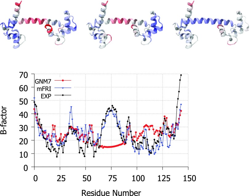
Nevertheless, there are structures for which FRI does not work either. In fact, structures that fail NMA and GNM are likely to be difficult for the original FRI method as well. One such structure is pictured in Figure 2 where the GNM method fails to predict the high flexibility of a hinge region in calmodulin with any cutoff distance. There are a number of reasons for this and other types of failure. Crystal environment, solvent type, co-factors, data collection conditions, and structural refinement procedures are well-known causes.^17,21,22,30

FIG. 2.

Top, the structure of calmodulin (PDB ID: 1CLL) visualized in Visual Molecular Dynamics (VMD)¹⁸ and colored by experimental B-factors (left), mFRI predicted B-factors (middle), and GNM predicted B-factors (right) with red representing the most flexible regions. Bottom, the experimental and predicted B-factor values plotted per residue. The GNM7 is for the GNM method with a cutoff distance of 7 Å. Clearly, GNM misses the flexible hinge region. The mFRI is parametrized at υ¹ = 3, η¹ = 3 Å, υ² = 3, η² = 7 Å, κ³ = 1, and η³ = 15 Å.

However, there is one more important cause that has not been discussed in the literature to our best knowledge, namely, multiple characteristic length scales in a single protein structure. Indeed, contrary to small molecules, macromolecular interactions have a wide variety of characteristic length scales, ranging from covalent bond, hydrogen bond, van der Waals bond, residue, alpha helix and beta sheet, domain, and protein scales. Protein flexibility is intrinsically associated with protein interactions and thus must have a multiscale trait as well. When the GNM or FRI method is parametrized at a given cutoff or scale parameter, it captures only a subset of the characteristic length scales but inevitably misses the other characteristic length scales of the protein. Consequently, none of them is able to provide an accurate B-factor prediction.

The multiscale flexibility-rigidity index (mFRI) is constructed to capture the multiscale collective motions of macromolecules. We utilize multiple correlation kernels, with each kernel being parametrized at specific scale to characterize the multiscale flexibility of macromolecules. The nth flexibility index of the ith (coarse-grained) particle is given by

$${\displaystyle f_i^n=\frac{1}{\sum _{j=1}^N\underset{j}{\overset{n}{w}}{\mathrm{\Phi }}^n(\Vert {\mathbf{r}}_i-{\mathbf{r}}_j\Vert ;{\eta }_j^n)},}$$ (1)

where $w_j^n$ is an atomic type dependent parameter, ${\mathrm{\Phi }}^n(\Vert {\mathbf{r}}_i-{\mathbf{r}}_j\Vert ;{\eta }_j^n)$ is a correlation kernel, and ${\eta }_j^n$ is a scale parameter. Here, r_i and r_j are the coordinates for ith and jth particles, respectively. We seek the minimization of the form

$${\displaystyle {\mathrm{Min}}_{a^n,b}\left\{\sum _i{\left|\sum _n{a}^n{f}_i^n+b-B_i^e\right|}^2\right\},}$$ (2)

where $\left\{B_i^e\right\}$ are the experimental B-factors. We use generalized exponential kernels^26,34

$${\displaystyle {\mathrm{\Phi }}^n(\Vert \mathbf{r}-{\mathbf{r}}_j\Vert ;{\eta }_j^n)=e^{-{\left(\Vert \mathbf{r}-{\mathbf{r}}_j\Vert /{\eta }_j^n\right)}^{\kappa }},\kappa >0}$$ (3)

and generalized Lorentz kernels

$${\displaystyle {\mathrm{\Phi }}^n(\Vert \mathbf{r}-{\mathbf{r}}_j\Vert ;{\eta }_j^n)=\frac{1}{1+{\left(\Vert \mathbf{r}-{\mathbf{r}}_j\Vert /{\eta }_j^n\right)}^{\upsilon }},\upsilon >0.}$$ (4)

In principle, all parameters can be optimized. For simplicity and computational efficiency, we only determine {aⁿ} and b in the above minimization process. In this work, we limit the number of kernels to at most three and set $w_j^n=1$. Both generalized exponential kernels and generalized Lorentz kernels are employed. More detailed description of the mFRI is given in the supplementary material.¹

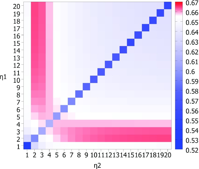
To understand the multiscale behavior of flexibility analysis, we consider a test set containing 364 protein structures whose Protein Data Bank (PDB) identities are listed in the literature²⁶ and it contains test sets used in GNM studies.²⁷ This test set omits one structure present in previous FRI studies (PDB ID: 1AGN) due to unrealistic B-factor data. Our goal is to examine how an additional kernel with a large length scale impacts the flexibility analysis. To this end, we consider two smooth Lorentz type of kernels with υ = 3. We explore a number of scale combinations as shown in Fig. 1, which plots the MCC values for B-factor prediction on the set of 364 structures. The low MCC values on the diagonal line indicate that two-scale methods are always better than a single scale one. The best results are achieved at the combination of a relatively small-scale kernel and a relatively large-scale kernel. This behavior proves the importance of incorporating multiscale in the biomolecular flexibility analysis. The best MCC for the test set is 0.67, which is about 20% better than the best GNM prediction and about 6% improvement over our single scale FRI approach.

FIG. 1.

An illustration of multiscale behavior in protein flexibility analysis. Two Lorentz kernels (υ = 3) are used. Their scale values, η values, are listed along the horizontal and vertical axes. The mean correlation coefficient value for B-factor prediction on a set of 364 proteins is shown in each cell of the matrix and color coded for convenience with red representing the highest correlation coefficients and green the lowest. Obvious, the combination of a relatively small-scale kernel and a relatively large-scale kernel delivers best prediction, which indicates the importance of incorporating multiscale in protein flexibility analysis.

The improvement in the MCC for B-factor prediction on a set of 364 proteins discussed above obscures the fact that the proposed multiscale method is able to capture the multiscale behaviors in many structures that fail the original FRI and GNM. In the rest of this paper, we demonstrate utility of the proposed multiscale method by a few case studies. A three-scale FRI is employed.

Protein hinge regions have been shown to be correlated with active sites and catalysis in enzymes. Flexibility has a major role in specificity of binding of a protein to other proteins, nucleic acids, or other molecules. An active site or docking region that is more flexible will accommodate more varied substrates or partners while more rigid domains are more specific. Protein hinges are also found separating large domains of proteins. In this context, the hinges can be very important for protein conformational changes. The protein featured in this section, calmodulin, is a good example of a hinge that affects both structure and function.

The central region of calmodulin shown in Figure 2 is a long α-helix which is unwound or kinked at the middle when no calcium is bound to the two distal metal coordinating domains. In both forms, with or without calcium bound, this helix retains a large degree of flexibility based on B-factor values from the PDB files (1CLL and 1CFD).

Many tools exist for the prediction and analysis of hinges in proteins using bioinformatics,¹³ graph theory,^11,20,28 and energetics.¹² The proposed mFRI has capabilities similar to those in these tools. The mFRI can be used to predict hinge regions by high FRI values or predicted B-values.

A comparison of mFRI method and GNM for the B-factor prediction of calcium-bound calmodulin is displayed in Figure 2. B-factor prediction by single kernel FRI and GNM is unable to accurately predict the hinge region in the middle of the protein with any parameter. Two- and three-kernel based mFRI methods, on the other hand, are much more accurate in the hinge region. As more kernels are added, the accuracy can be seen to grow but sufficient accuracy is achieved at three kernels.

We have shown in our supplementary material¹ that a similarly good B-factor prediction for calmodulin type of structures can be achieved by the original FRI method if the crystal effect is taken into consideration. This result suggests that the proposed mFRI method may be able to take care some crystal effects.

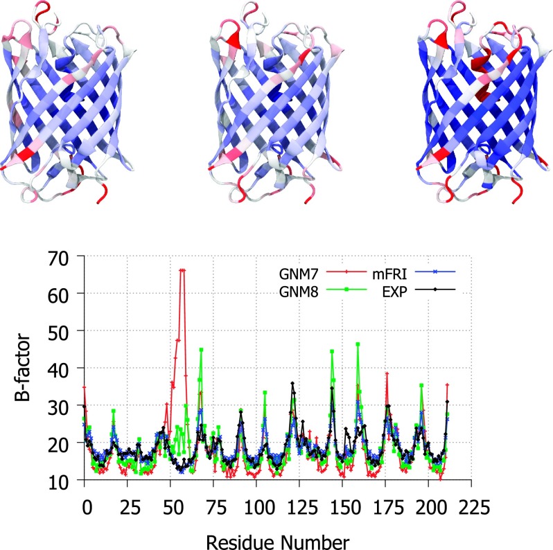
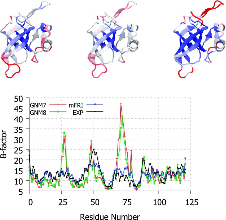
Cyan fluorescent protein (CFP), shown in Figure 3, is a homolog of the famous green fluorescent protein (GFP). Isolated from the crystal jellyfish in the 1990s,²⁹ GFP enabled a revolution in biochemistry by allowing the tagging and tracking of a wide range of molecules. CFP was found later in Anthozoa coral species which have turned out to be a good source of fluorescent proteins with varied emission spectra.²⁵ In this example, we examine the flexibility of an engineered CFP from Clavularia coral² (PDB ID: 2HQK), mTFP1. It is clear in Figure 3 that GNM B-factor predictions contain a large error around residues 50-60 which is very pronounced at the recommended cutoff of 7 Å and is still somewhat problematic when the cutoff is changed to 8 Å, the best alternate parameter found by searching incrementally outward from 7 Å in either direction. mFRI on the other hand has no issue with this particular region. Upon further inspection, it is clear that the offending region is the small, alpha-helical region suspended in the center of the beta-barrel. It is not surprising that this sort of configuration would be highly cutoff parameter dependent in a scheme such as GNM, which has hard cutoffs for connectivity. It would appear that this structure is dominated by short range interaction but the region of residues 50-60 is affected to a large degree by mid-range interactions, i.e., there are at least two important scales of interaction in this case. It follows then that mFRI, which has kernels to capture short- and mid-range interactions, would perform better than GNM7 or GNM8 parameterizations alone in B-factor predictions, Figure 3, which is exactly what we see from the results.

FIG. 3.

Top, a visual comparison of experimental B-factors (left), mFRI predicted B-factors (middle), and GNM predicted B-factors (right) for the engineered cyan fluorescent protein, mTFP1 (PDB ID:2HQK). Bottom, the experimental and predicted B-factor values plotted per residue. The GNM naming convention indicates the cutoff used for the GNM method in Å, i.e., GNM7 is the GNM method with a cutoff distance of 7 Å.

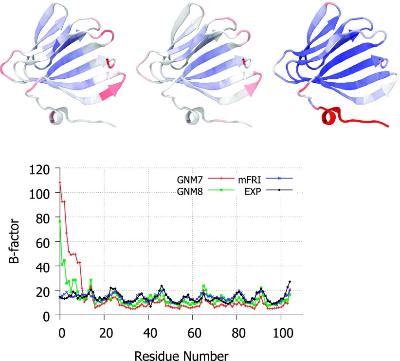
A similar situation exists with the structure 1V70, a probable antibiotic synthesis protein, which is shown in Figure 4. As in the last example, the problematic portion for B-factor prediction comes at the end of a protein chain. In this case, there is an overestimation of flexibility for residues 1-10 when using GNM. Again, varying parameters from the recommended 7 Å results in marginally better results; however, no parametrization is able to reach the accuracy of mFRI.

FIG. 4.

Top, a visual comparison of experimental B-factors (left), mFRI predicted B-factors (middle), and GNM predicted B-factors (right) for a probable antibiotic synthesis protein (PDB ID:1V70). Bottom, the experimental and predicted B-factor values plotted per residue.

The final example is a biologically important molecule, ribosomal protein L14, a component of the 60S ribosomal subunit.⁸ Depicted in Figure 5, L14 is a structurally diverse protein containing regions of alpha helix, beta-barrel, parallel beta strands, and a beta-hairpin motif. The pattern of flexibility predicted by GNM for this structure is shown to be over-exaggerated, i.e., rigid areas are predicted to be more rigid than they actually are and vice versa. This pattern exists in most GNM results due to the use of a hard cutoff in the Kirchhoff matrix. Such a hard cutoff will inevitably lead to the overestimation of bond importance near the edge of the cutoff; therefore, if a large number of interactions exist for a particular atom near the cutoff point, there is likely to be a large error in the estimation of flexibility for that atom. This is likely what is happening with the errors in GNM calculation of the proteins in Figures 3–5; the protein at the end of the chain may be near the edge of the cutoff distance for many interactions with the bulk of the proteins. While adjusting GNM’s cutoff distance may temper the error being introduced, it cannot eliminate it completely unless they change to a soft-decaying kernel method such as FRI. Nevertheless, soft-decaying kernel based methods can only alleviate the problem. They do not deliver satisfactory B-factor predictions unless a multiscale strategy is employed. We note that it is not obvious how to incorporate a multiscale strategy in matrix diagonalization based methods.

FIG. 5.

Top, a visual comparison of experimental B-factors (left), mFRI predicted B-factors (middle), and GNM predicted B-factors (right) for the ribosomal protein L14 (PDB ID:1WHI). Bottom, the experimental and predicted B-factor values plotted per residue.

REFERENCES

- 1.See supplementary material at http://dx.doi.org/10.1063/1.4922045 E-JCPSA6-142-044522 for theoretical formulation, parametrization, efficiency test, additional examples, and crystal packing effects.
- 2.Ai H. W., Henderson J., Remington S., and Campbell R., “Directed evolution of a monomeric, bright and photostable version of clavularia cyan fluorescent protein: Structural characterization and applications in fluorescence imaging,” Biochem. J 400, 531–540 (2006). 10.1042/BJ20060874 [DOI] [PMC free article] [PubMed] [Google Scholar]
- 3.Allen M. P. and Tildesley D. J., Computer Simulation of Liquids (Clarendon Press, Oxford, 1987). [Google Scholar]
- 4.Atilgan A. R., Durrell S. R., Jernigan R. L., Demirel M. C., Keskin O., and Bahar I., “Anisotropy of fluctuation dynamics of proteins with an elastic network model,” Biophys. J. 80, 505 – 515 (2001). 10.1016/S0006-3495(01)76033-X [DOI] [PMC free article] [PubMed] [Google Scholar]
- 5.Bahar I., Atilgan A. R., Demirel M. C., and Erman B., “Vibrational dynamics of proteins: Significance of slow and fast modes in relation to function and stability,” Phys. Rev. Lett. 80, 2733 – 2736 (1998). 10.1103/PhysRevLett.80.2733 [DOI] [Google Scholar]
- 6.Bahar I., Atilgan A. R., and Erman B., “Direct evaluation of thermal fluctuations in proteins using a single-parameter harmonic potential,” Folding Des. 2, 173 – 181 (1997). 10.1016/S1359-0278(97)00024-2 [DOI] [PubMed] [Google Scholar]
- 7.Brooks B. R., Bruccoleri R. E., Olafson B. D., States D., Swaminathan S., and Karplus M., “Charmm: A program for macromolecular energy, minimization, and dynamics calculations,” J. Comput. Chem. 4, 187–217 (1983). 10.1002/jcc.540040211 [DOI] [Google Scholar]
- 8.Davies C., White S. W., and Ramakrishnan V., “The crystal structure of ribosomal protein l14 reveals an important organizational component of the translational apparatus,” Structure 4(1), 55–66 (1996). 10.1016/S0969-2126(96)00009-3 [DOI] [PubMed] [Google Scholar]
- 9.Demerdash O. N. A. and Mitchell J. C., “Density-cluster NMA: A new protein decomposition technique for coarse-grained normal mode analysis,” Proteins: Struct., Funct., Bioinf. 80(7), 1766–1779 (2012). 10.1002/prot.24072 [DOI] [PubMed] [Google Scholar]
- 10.Dudko O. K., Hummer G., and Szabo A., “Intrinsic rates and activation free energies from single-molecule pulling experiments,” Phys. Rev. Lett. 96, 108101 (2006). 10.1103/PhysRevLett.96.108101 [DOI] [PubMed] [Google Scholar]
- 11.Emekli U., Dina S., Wolfson H., Nussinov R., and Haliloglu T., “HingeProt: Automated prediction of hinges in protein structures,” Proteins 70(4), 1219–1227 (2008). 10.1002/prot.21613 [DOI] [PubMed] [Google Scholar]
- 12.Flores S. and Gerstein M., “FlexOracle: Predicting flexible hinges by identification of stable domains,” BMC Bioinf. 8(1), 215 (2007). 10.1186/1471-2105-8-215 [DOI] [PMC free article] [PubMed] [Google Scholar]
- 13.Flores S., Lu L., Yang J., Carriero N., and Gerstein M., “Hinge atlas: Relating protein sequence to sites of structural flexibility,” BMC Bioinf. 8, 167 (2007). 10.1186/1471-2105-8-167 [DOI] [PMC free article] [PubMed] [Google Scholar]
- 14.Frauenfelder H., Slihar S. G., and Wolynes P. G., “The energy landsapes and motion of proteins,” Science 254(5038), 1598–1603 (1991). 10.1126/science.1749933 [DOI] [PubMed] [Google Scholar]
- 15.Go N., Noguti T., and Nishikawa T., “Dynamics of a small globular protein in terms of low-frequency vibrational modes,” Proc. Natl. Acad. Sci. U. S. A. 80, 3696 – 3700 (1983). 10.1073/pnas.80.12.3696 [DOI] [PMC free article] [PubMed] [Google Scholar]
- 16.Hinsen K., “Analysis of domain motions by approximate normal mode calculations,” Proteins 33, 417 – 429 (1998). 10.1002/(SICI)1097-0134(19981115)33:3%3C417::AID-PROT10%3E3.0.CO;2-8 [DOI] [PubMed] [Google Scholar]
- 17.Hinsen K., “Structural flexibility in proteins: Impact of the crystal environment,” Bioinformatics 24, 521 – 528 (2008). 10.1093/bioinformatics/btm625 [DOI] [PubMed] [Google Scholar]
- 18.Humphrey W., Dalke A., and Schulten K., “VMD – visual molecular dynamics,” J. Mol. Graphics 14(1), 33–38 (1996). 10.1016/0263-7855(96)00018-5 [DOI] [PubMed] [Google Scholar]
- 19.Jacobs D. J., Rader A. J., Kuhn L. A., and Thorpe M. F., “Protein flexibility predictions using graph theory,” Proteins: Struct., Funct., Genet. 44(2), 150–165 (2001). 10.1002/prot.1081 [DOI] [PubMed] [Google Scholar]
- 20.Keating K. S., Flores S. C., Gerstein M. B., and Kuhn L. A., “StoneHinge: Hinge prediction by network analysis of individual protein structures,” Protein Sci. 18(2), 359–371 (2009). 10.1002/pro.38 [DOI] [PMC free article] [PubMed] [Google Scholar]
- 21.Kondrashov D. A., Van Wynsberghe A. W., Bannen R. M., Cui Q., and Phillips J. G. N., “Protein structural variation in computational models and crystallographic data,” Structure 15, 169 – 177 (2007). 10.1016/j.str.2006.12.006 [DOI] [PMC free article] [PubMed] [Google Scholar]
- 22.Kundu S., Melton J. S., Sorensen D. C., and Phillips J. G. N., “Dynamics of proteins in crystals: Comparison of experiment with simple models,” Biophys. J. 83, 723 – 732 (2002). 10.1016/S0006-3495(02)75203-X [DOI] [PMC free article] [PubMed] [Google Scholar]
- 23.Levitt M., Sander C., and Stern P. S., “Protein normal-mode dynamics: Trypsin inhibitor, crambin, ribonuclease and lysozyme,” J. Mol. Biol. 181(3), 423 – 447 (1985). 10.1016/0022-2836(85)90230-X [DOI] [PubMed] [Google Scholar]
- 24.Li G. H. and Cui Q., “A coarse-grained normal mode approach for macromolecules: An efficient implementation and application to Ca(2+)-ATPase,” Bipohys. J. 83, 2457 – 2474 (2002). 10.1016/S0006-3495(02)75257-0 [DOI] [PMC free article] [PubMed] [Google Scholar]
- 25.Matz M. V., Fradkov A. F., Labas Y. A., Savitsky A. P., Zaraisky A. G., Markelov M. L., and Lukyanov S. A., “Fluorescent proteins from nonbioluminescent anthozoa species,” Nat. biotechnol. 17(10), 969–973 (1999). 10.1038/13657 [DOI] [PubMed] [Google Scholar]
- 26.Opron K., Xia K. L., and Wei G. W., “Fast and anisotropic flexibility-rigidity index for protein flexibility and fluctuation analysis,” J. Chem. Phys. 140, 234105 (2014). 10.1063/1.4882258 [DOI] [PMC free article] [PubMed] [Google Scholar]
- 27.Park J. K., Jernigan R., and Wu Z., “Coarse grained normal mode analysis vs. refined Gaussian network model for protein residue-level structural fluctuations,” Bull. Math. Biol. 75, 124 – 160 (2013). 10.1007/s11538-012-9797-y [DOI] [PMC free article] [PubMed] [Google Scholar]
- 28.Shatsky M., Nussinov R., and Wolfson H. J., “FlexProt: Alignment of flexible protein structures without a predefinition of hinge regions,” J. Comput. Biol. 11(1), 83–8106 (2004). 10.1089/106652704773416902 [DOI] [PubMed] [Google Scholar]
- 29.Shimomura O., Johnson F. H., and Saiga Y., “Extraction, purification and properties of aequorin, a bioluminescent protein from the luminous hydromedusan, aequorea,” J. Cell. Comp. Physiol. 59(3), 223–239 (1962). 10.1002/jcp.1030590302 [DOI] [PubMed] [Google Scholar]
- 30.Song G. and Jernigan R. L., “vgnm: A better model for understanding the dynamics of proteins in crystals,” J. Mol. Biol. 369(3), 880 – 893 (2007). 10.1016/j.jmb.2007.03.059 [DOI] [PMC free article] [PubMed] [Google Scholar]
- 31.Tama F., Gadea F. X., Marques O., and Sanejouand Y. H., “Building-block approach for determining low-frequency normal modes of macromolecules,” Proteins: Struct., Funct., Bioinf. 41(1), 1–7 (2000). 10.1002/1097-0134(20001001)41:1%3C1::AID-PROT10%3E3.0.CO;2-P [DOI] [PubMed] [Google Scholar]
- 32.Tama F. and Sanejouand Y. H., “Conformational change of proteins arising from normal mode calculations,” Protein Eng. 14, 1 – 6 (2001). 10.1093/protein/14.1.1 [DOI] [PubMed] [Google Scholar]
- 33.Tasumi M., Takenchi H., Ataka S., Dwidedi A. M., and Krimm S., “Normal vibrations of proteins: Glucagon,” Biopolymers 21, 711 – 714 (1982). 10.1002/bip.360210318 [DOI] [PubMed] [Google Scholar]
- 34.Xia K. L., Opron K., and Wei G. W., “Multiscale multiphysics and multidomain models — Flexibility and rigidity,” J. Chem. Phys. 139, 194109 (2013). 10.1063/1.4830404 [DOI] [PMC free article] [PubMed] [Google Scholar]
- 35.Xia K. L. and Wei G. W., “A stochastic model for protein flexibility analysis,” Phys. Rev. E 88, 062709 (2013). 10.1103/PhysRevE.88.062709 [DOI] [PubMed] [Google Scholar]
- 36.Xia K. L. and Wei G. W., “Molecular nonlinear dynamics and protein thermal uncertainty quantification,” Chaos 24, 013103 (2014). 10.1063/1.4861202 [DOI] [PMC free article] [PubMed] [Google Scholar]
Associated Data
This section collects any data citations, data availability statements, or supplementary materials included in this article.
Data Citations
- See supplementary material at http://dx.doi.org/10.1063/1.4922045 E-JCPSA6-142-044522 for theoretical formulation, parametrization, efficiency test, additional examples, and crystal packing effects.