A comparison of weighted ensemble and Markov state model methodologies

Abstract

Computation of reaction rates and elucidation of reaction mechanisms are two of the main goals of molecular dynamics (MD) and related simulation methods. Since it is time consuming to study reaction mechanisms over long time scales using brute force MD simulations, two ensemble methods, Markov State Models (MSMs) and Weighted Ensemble (WE), have been proposed to accelerate the procedure. Both approaches require clustering of microscopic configurations into networks of “macro-states” for different purposes. MSMs model a discretization of the original dynamics on the macro-states. Accuracy of the model significantly relies on the boundaries of macro-states. On the other hand, WE uses macro-states to formulate a resampling procedure that kills and splits MD simulations for achieving better efficiency of sampling. Comparing to MSMs, accuracy of WE rate predictions is less sensitive to the definition of macro-states. Rigorous numerical experiments using alanine dipeptide and penta-alanine support our analyses. It is shown that MSMs introduce significant biases in the computation of reaction rates, which depend on the boundaries of macro-states, and Accelerated Weighted Ensemble (AWE), a formulation of weighted ensemble that uses the notion of colors to compute fluxes, has reliable flux estimation on varying definitions of macro-states. Our results suggest that whereas MSMs provide a good idea of the metastable sets and visualization of overall dynamics, AWE provides reliable rate estimations requiring less efforts on defining macro-states on the high dimensional conformational space.

I. INTRODUCTION

Computation of reaction rates in the context of molecular dynamics (MD) has given rise to an outstanding number of publications over the past decades. Although it is possible to characterize reaction rates from a theoretical standpoint, accurate computations of the corresponding quantities by classical numerical methods turn out to be very costly as the size of the molecule increases. Therefore, a host of numerical methods designed to improve the efficiency of such computations have been developed. We refer to Ref. 1 for a comprehensive survey.

Herein, we compare two methodologies that have attracted attention over the past few years: the so-called Weighted Ensemble (WE) and Markov State Models (MSMs) methodologies (as an example, see Refs. ^2–5 and Refs. ^6–8, respectively). Both of these methodologies rely on some underlying coarse partition of the state space. Thereby is meant that the state space, the set of microscopic configurations characterizing the molecule’s state, is split into a collection of subsets, the so-called macro-states, each of which gathers close microscopic configurations. Such macro-states are then used to speed up or, equivalently, lower the cost of reaction rates computations.

The ways MSMs and WE methodologies make use of this partition are very different. In the former case, it is used to build some coarse dynamics from statistics collected over short-time trajectories of the original system. The resulting representation of the system’s behavior is a reduced dynamics on the collection of macro-states. The reaction rate of the original dynamics is then approximated by that of the coarse one. In the latter case, the perspective is somehow different. WE methodologies do not involve such a thing as a reduced dynamics. They are intrinsically based on the simulation of multiple replicas of the original microscopic dynamics over long time intervals. The coarse partition is used in such a way as to maintain the number of replicas in each macro-state approximatively constant along the simulation. At fixed computational cost, this is achieved in an unbiased manner by killing or merging replicas at fixed deterministic times whilst allowing these replicas to carry different probabilistic weights, a step which is referred to as resampling. The resulting collection of correlated trajectories together with their final probabilistic weights is then used to compute any macroscopic property of the system that can be expressed as an average with respect to the equilibrium distribution. When defined in terms of flux, the reaction rate is such a property.

In this paper, we study the way the definition of the underlying coarse partition affects the accuracy of both methods. This is a crucial point since, in the case of complex molecules, such a partition is necessarily rather coarse due to the limited sampling on the high dimensional conformational space. Note that, in addition, the degree of coarseness being fixed, there are still many possible choices of partition left that correspond to different possible locations of macro-states boundaries. We will, thus, aim at understanding in both frameworks the way such parameters, global coarseness, and macro-state boundary locations alter the accuracy of reaction rates computations. We show that WE methodologies are less sensitive than MSMs methodologies to the definition of the underlying macro-states.

In the context of MSMs as well as in the case of WE methodologies, the several intrinsic sources of errors likely to be modified by changes of the underlying partition are singled out. On that ground, rigorous numerical experiments are carried over in the case of two very simple protein-like molecules, alanine dipeptide and penta-alanine. They illustrate the fact that, having a definition of underlying fine partition, both WE and MSMs generate good reaction rate estimations that lie in reference confidence interval computed using brute force method. However, accuracy of reaction rates computed from MSMs does not maintain if incorrectly splitting the state space, whereas WE estimations remain reliable on varying definitions of macro-states.

The outline of the article is as follows. In Sec. II, the general mathematical framework is first recalled. The partition’s influence on reaction rates computations is studied in each case. Section III focuses on the case of Markov state models. It recalls the way such reduced models are built and how such a building results in two main sources of error in reaction rates estimation. Section IV deals specifically with WE methodologies. It sums up the expected properties of such methods and investigates as well the way their performance depends on the underlying partition. In this article, we concentrate on a particular version of the Accelerated Weighted Ensemble (AWE) methodology. It is based on two features: the use of colors to differentiate walkers and that of resampling as already briefly mentioned above. Contrary to the case of MSMs, there is only one kind of error in the case of AWE: the statistical variance. Section V compares accuracy of folding rates estimated by AWE and MSM, considering two molecules: alanine dipeptide and penta-alanine. It is shown that, in the case when the partition is coarse (a situation consistent with numerical practice), the location of boundaries is the crucial determinant of accuracy of MSMs. On the other hand, refinements and shifts of the underlying coarse partition have little influence on the accuracy of the reaction rates estimates from AWE.

II. THE UNDERLYING DIFFUSION

In this paper, we shall only consider the case when the behavior of the underlying molecule is governed by the Langevin dynamics. The state of the molecule at time t is denoted by $(Q_t,P_t)\in {\left({\mathbb{R}}_q^3\right)}^d\times {\left({\mathbb{R}}_p^3\right)}^d$ where d denotes the number of atoms. For any 1 ≤ i ≤ d, variables $Q_t^i\in {\mathbb{R}}_q^3$ and $P_t^i\in {\mathbb{R}}_p^3$ refer to the position and momentum of the ith atom, respectively. The trajectory of the whole system is thus defined as the solution of the following system of Stochastic Differential Equations (SDE):

$${\displaystyle \left\{\begin{array}{l}d{Q}_t=M^{-1}{P}_{t}dt\hfill \\ d{P}_t=-\nabla V\left(Q_t\right)dt-\gamma M^{-1}{P}_{t}dt+\sqrt{\frac{2\gamma }{\beta }}d{W}_t\hfill \end{array},\right.}$$ (1)

where M denotes the mass matrix, γ is the friction parameter and β = 1/(k_BT) with k_B and T referring to the Boltzmann constant and temperature, respectively. Process (W_t)_t≥0 is a Brownian motion on ℝ^3d. The process (Q_t, P_t)_t≥0 is Markovian. Detailed discussion on its infinitesimal generator is included in Appendix A.

In practice, we do not deal with process (Q_t, P_t)_t≥0 itself but with some discrete-time approximation of it resulting from some discretization scheme of Eq. (1), namely, ${(Q_t^{\delta t},P_t^{\delta t})}_{t\ge 0}$ where δt denotes the time step of the discretization.

III. MARKOV STATE MODELS

A. Principle and related errors

1. Principle

The main idea behind MSMs is that the exact dynamics of the system can be approximated by a reduced model that relies on a coarse partition of the underlying state space. Most often, this partition involves only position variables. In other words, it is assumed that the behavior of the physical system can be studied by focusing on clusters of microscopic configurations, the so-called macro-states or cells. The coarse partition is thus defined as a collection of N_S subsets of ${\mathbb{R}}_q^{3d}$ (the macro-states) denoted by $\mathrm{\Pi }≔\left\{S_1,\dots ,S_{N_S}\right\}$. It satisfies

$${\displaystyle \forall 1\le i\ne j\le N_S,S_i\cap S_j=0̸\text{and}{\cup }_{1\le i\le N_S}{S}_i={\mathbb{R}}_q^{3d}.}$$ (2)

From the original continuous-time dynamics, a Markov chain on state space Π is built. Its transition matrix $\mathcal{P}={\left({\mathcal{P}}_{ij}\right)}_{1\le i,j\le N_S}$ is inferred from short-time simulations of the original system under ℙ_ρ (that is at equilibrium). In brief, we have

$${\displaystyle {\mathcal{P}}_{ji}={\mathcal{P}}_{ji}\left(\tau \right)={\mathbb{P}}_{\rho }(Q_{\tau }\in S_j|Q_0\in S_i),}$$ (3)

where τ is referred to as the lag time. Since this is a simple low-dimensional dynamics, given the two metastable states A and B, forward and backward fluxes can be computed exactly using transition path theory (see Ref. 9). The way to proceed can be described very briefly. First from the approximate transition matrix $\mathcal{P}\left(\tau \right)$, a new matrix is built L(τ) ≔ 𝒫(τ) − 𝕀_NS. In the case when one aims at computing the forward flux, that is the flux from A to B, the following linear system is solved:

$${\displaystyle \{\begin{array}{ll}{\sum }_{k=1}^{N_S}{L}_{ik}\left(\tau \right)f_k\left(\tau \right)=-\tau \hfill & \text{if }i\in S\setminus N\left(B\right)\hfill \\ f_i\left(\tau \right)=0\hfill & \text{if }i\in N\left(B\right)\hfill \end{array},}$$

where $N\left(B\right)\subset S≔\left\{1,\dots ,N_S\right\}$ denotes the set of indexes of macro-states whose union is equal to B. When parameter τ is small enough, the forward flux can then be computed as the inverse of the mean first passage

$${\displaystyle {\nu }_R^{A\to B}\left(\tau \right)≔{\left(\sum _{i\in N\left(A\right)}{\left(V_1\left(\tau \right)\right)}_i{f}_i\left(\tau \right)\right)}^{-1},}$$

where V₁ still denotes the equilibrium distribution associated to $\mathcal{P}\left(\tau \right)$ (its first eigenvector properly renormalized) and N(A) the set of indexes of macro-states whose union is A. Of course, the approximate backward flux ${\nu }_R^{B\to A}\left(\tau \right)$ can be computed in a similar manner.

In the very general case, when partition Π is refined uniformly, ν_R(τ) tends to the exact value ν_R. However, such a uniform refinement is not necessary. In particular, if there is any information available about some privileged directions or reaction paths, refining the partition along these is often sufficient to guarantee the convergence to the exact value.

2. Empirical estimators

It is clear from the previous paragraph that MSMs are intrinsically biased. The underlying partition at the very basis of these methodologies results in a deterministic error ν_R − ν_R(τ). In practice, this is not the only source of error. One has to cope as well with statistical error resulting from finite sampling of the system. There are several ways to approximate the transition matrix (3).

A most general method can be described in the following manner. Suppose that we are possessed of M independent trajectories of the system on time interval $\left[0,T\right]$ with T > τ. We seek to estimate ${\mathcal{P}}_{ji}$, that is the probability that a walker initially within state S_i be in S_j at time t = τ. For all trajectories, we first compute the average number of transitions achieved from S_i to S_j over time intervals of length τ. More precisely, it is estimated by

$${\displaystyle C_{ji}(\tau ,\omega )=\frac{1}{T-\tau }\sum _{k=1}^M\sum _{s=0}^{T-\tau }{\mathbf{1}}_{\left\{\underset{s}{\overset{k}{Q}}\in S_i,Q_{s+\tau }^k\in S_j\right\}}\left(\omega \right),}$$ (4)

where ω indicates that this transition count is estimated by discrete time approximation of Langevin dynamics equation (1), ${\left\{{\left(Q_t^k\right)}_{0\le t\le T}\right\}}_{1\le k\le M}$ denotes the set of M independent replicas already mentioned. 1_{⋅} is equal to 1 if the statement { ⋅ } is true, 0 otherwise. Transition probability ${\mathcal{P}}_{ji}(\tau ,\omega )$ is equal to the transition count C_ji(τ, ω) divided by the total amount of time spent in S_j,

$${\displaystyle {\mathcal{P}}_{ji}(\tau ,\omega )=\frac{C_{ji}(\tau ,\omega )}{\sum _{k=1}^{N_s}{C}_{ki}(\tau ,\omega )}.}$$

Because dynamics equation (1) is reversible, it is further assumed that the MSMs shall satisfy the detailed balance condition. An improved estimator (originating from Ref. 10) of transition probability is

$${\displaystyle {\mathcal{P}}_{ji}(\tau ,\omega )=\frac{C_{ji}(\tau ,\omega )+C_{ij}(\tau ,\omega )}{\sum _{k=1}^{N_s}{C}_{ki}(\tau ,\omega )+C_{ik}(\tau ,\omega )}.}$$ (5)

In the end, the approximate value of the reaction rate is then ν_R(τ, ω), which is calculated from L(τ, ω) ≔ 𝒫(τ, ω) − 𝕀_NS.

3. Structure of the error

The total error for this class of methods can be decomposed in the following manner:

$${\displaystyle {\nu }_R-{\nu }_R(\tau ,\omega )=({\nu }_R-{\nu }_R\left(\tau \right))+\left({\nu }_R\left(\tau \right)-{\nu }_R(\tau ,\omega )\right).}$$

There are thus two types of error.

• •The term e₁(Π, τ) ≔ ν_R − ν_R(τ) is the structural error related to the Markov state models methodology. It is related both to the nature of the coarse partition Π and to the presence of τ. It decays when the partition is refined. The related convergence analysis can be found in Refs. ¹¹ and ¹².
• •The term e₂(Π, τ, ω) ≔ ν_R(τ) − ν_R(τ, ω) will be referred to as the statistical error. Its variance is related to the width of some confidence interval. To quantify this kind of error, we can separate the MD trajectories into blocks and build multiple MSMs. The statistical error is estimated by a constant times standard deviation of ν_R(τ)’s estimated from all MSMs.

IV. AWE METHODOLOGY

A. Principle and related errors

Weighted ensemble methodologies date back to the seminal work in Ref. 2. The reaction rate is defined as the average number of trajectories originating from the reactant state $A\subset {\mathbb{R}}_q^{3d}$ that enter the product space $B\subset {\mathbb{R}}_q^{3d}$ per unit of time. In Ref. 2, the first version of the weighted ensemble methodology was applied to the case of an out-of-equilibrium system. The key idea of Ref. 2 is that of resampling. Such a procedure relies on a coarse partition Π that satisfies Eq. (2). Roughly speaking, resampling is a procedure that, at some deterministic times, either kills or merges replicas in each macro-state, depending on whether such a macro-state is depleted or not. It does not result in any bias because replicas are allowed to carry different probabilistic weights. Note that, as a matter of fact, there are numerous ways to adapt this general idea. It has already been applied to a wide range of situations (see Refs. ^{4, 13}, and ¹⁴, for instance) and, indeed, several versions of it have been developed (see Ref. 3). In addition, it has been shown that it can indeed be applied to a class of underlying dynamics broader than expected (see Ref. 15).

The version we are going to focus on in this section originates from Ref. 1. It is closely related to the one studied in Ref. 16. It couples two features: that of resampling as afore described and that of colors, which is involved in the very definition of the reaction rate in terms of trajectories when no information about the past is available at time t = 0. More details about both are provided in the following. We refer the reader interested in a more mathematical treatment of these issues to Refs. ¹⁷ and ¹⁸.

1. Colors

The reaction rate is defined as the average number of independent trajectories originating from A that enter B per unit of time. It is the flux of replicas coming from A through the boundary of B. As a consequence, in order to estimate the reaction rate at some fixed time, we need information about both the current positions of replicas and the metastable sets they come from (either A or B). The latter is an information about the past of trajectories.

To keep track of it, an additional state variable has to be introduced. This variable will be referred to as the color of a replica (the term label is sometimes used as well). The color associated to trajectory (Q_t, P_t)_t≥0 is denoted by (I_t)_t≥0. It is a stochastic process such that, for t ≥ 0, I_t = − 1 if the last metastable state visited by the trajectory is A and I_t = 1 otherwise (the trajectory comes from B). The replica will be said to be blue in the first case, red in the second. The reaction rate is then the average flux of blue replicas across the boundary of B per unit of time. The main difficulty linked with this formalism is that at time t = 0, there is no natural manner to provide replicas in ${\mathbb{R}}_q^{3d}\setminus (A\cup B)$ with some color. Here, we will choose one based on an initial distribution ${\tilde{\mu }}_0(dq\times dp\times di)$ (di refers to the canonical measure on { − 1, 1}) that stands for the push-forward measure of (Q₀, P₀, I₀). Process (I_t)_t≥0 is then well-defined at all times.

The color method improves the WE method proposed in Ref. 2, in which framework, each time a replica crosses the boundary of B, it is killed and a new replica is issued on the boundary of A: there are only blue walkers. This approach in Ref. 2 has a drawback: the proper way to create new walkers on the boundary of A is unknown. It has, thus, to be somehow estimated, which may result in a bias. The color formalism does not require such a hypothesis. The way blue walkers are created on the boundary of A is exact: it coincides with the distribution of red walkers entering A. In this context, whatever the initial distribution ${\tilde{\mu }}_0(dq\times dp\times di)$, after some time, the system as a whole will reach some equilibrium characterized by a distribution $\tilde{\rho }(dq\times dp\times di)$ related to ρ and the forward committor function (see Ref. 19). At equilibrium, two coupled out-of-equilibrium systems compensate: the one associated to the dynamics of blue replicas and the one associated to red ones. As a consequence, this framework allows one to compute, in an unbiased manner, quantities such as forward and backward fluxes or free energy to which the out-of-equilibrium systems described in Ref. 2 do not give any access.

2. Fluxes

Now that the concept of colors has been explained, we can provide a more mathematical definition of the instantaneous flux. For sake of simplicity, we will work with the discrete time approximation ${(Q_n^k,P_n^k,I_n^k)}_{0\le n\le T,1\le k\le M}$. It is possible to define the instantaneous flux in the case of the continuous-time dynamics, but such a definition gives rise to unnecessary technicalities. Suppose then that M independent replicas of the discrete time dynamics with time step δt are run in parallel. The instantaneous flux at time t = (n + 1) δt can be defined as

$${\displaystyle {\varphi }_{n+1}\left(\omega \right)=\frac{1}{M\delta t}{\sum }_{k=1}^M{\mathbf{1}}_{\left\{\mathrm{\Delta }{I}_{n+1}^k=2\right\}}\left(\omega \right),}$$

where

$${\displaystyle \mathrm{\Delta }{I}_{n+1}^k=I_{n+1}^k-I_n^k.}$$ (6)

Event $\left\{\mathrm{\Delta }{I}_{n+1}^k=2\right\}$ means the kth walker enters B at time t = (n + 1) δt and it originates from A.

Practically, the first few samples are often biased because of an approximate choice of colors at t = 0. Therefore, when computing the average using N samples, the first n₁ are discarded. We will denote ${\overline{\varphi }}_n\left(\omega \right)$ the average obtained using M replicas and n time steps,

$${\displaystyle {\overline{\varphi }}_n\left(\omega \right)=\frac{1}{n-n_1+1}\sum _{k=n_1}^n{\varphi }_k\left(\omega \right).}$$

But the mean of the instantaneous flux is not the only information we are interested in. We would also like to estimate its variance. However, the successive elements of the flux time series are often correlated; the standard variance estimator is therefore inappropriate. To get rid of correlation effects, a block-averaging technique (see Ref. 20 for more details) is applied. The number of blocks involved is denoted by N_b and is such that (T − t₁)/N_b is an integer. In the following, the corresponding variance estimate is denoted by Σ_Nb(ϕ). As a result, we are left with the following global estimate:

$${\displaystyle {\widehat{\nu }}_R\approx {\overline{\varphi }}_n\left(\omega \right)\pm \mathrm{constant}\ast \sqrt{{\mathrm{\Sigma }}_{N_b}\left(\varphi \left(\omega \right)\right)}}$$

that embodies informations about both the average and the variance of the instantaneous flux. The constant is set to 1.5 for estimating the 90% confidence interval.

In the case of forward and backward fluxes, the methodology is similar. In the former case, as an example, the estimators described above build on the time-series of instantaneous forward fluxes

$${\displaystyle {\varphi }_{n+1}^{A\to B}\left(\omega \right)=\frac{{\varphi }_{n+1}\left(\omega \right)\cdot M}{\left(\sum _{k=1}^M{\mathbf{1}}_{\left\{\underset{n}{\overset{k}{I}}=-1\right\}}\left(\omega \right)\right)}.}$$

The instantaneous forward flux is the percentage of blue walkers that enter B at time t = nδt.

3. Resampling

We now consider the methodology proposed in Ref. 1. At the bottom of it, there are two peculiar features: a new resampling algorithm and the fact that such an algorithm is applied to both colors. In the following, we briefly describe the several steps characterizing this particular version of WE.

Let us first give ourselves some parameter τ₁ > 0 referred to as the resampling time. At time t = 0, we consider M = N_S × 2N_C independent replicas of the system whose positions within the extended state space ${\mathbb{R}}_q^{3d}\times {\mathbb{R}}_p^{3d}\times \left\{-1,1\right\}$ are chosen in the following manner. In each one of the N_S macro-states associated to the coarse partition Π, we initially generate 2N_C replicas, the positions of which are distributed according to equilibrium distribution. For sake of simplicity, we will consider that, for cells in ${\mathbb{R}}_q^{3d}\setminus (A\cup B)$, half of these replicas are blue. Each replica is assigned a weight, which is equal to the normalized equilibrium population of its macro-state divided by 2N_C.

All replicas are then run independently till time t = τ₁. At that time, the resampling procedure is applied based on positions of replicas. In each cell, replicas are duplicated, killed, or merged in order to preserve a constant number of walkers of each color. The number of new replicas generated from an old one is in average proportional to its relative probabilistic weight (that is its contribution to the total weight of cell S_k at $t={\tau }_1^{-}$). In addition, in each cell S_k, for each color, all new replicas are given the same new probabilistic weight. This weight is equal to the total weight of the cell at t = τ₁ (the sum of all the weights of replicas in S_k) divided by N_C (the target number of replicas for each color). Once the resampling step is over, that is, once the new sample and its associated probabilistic weights have been computed, the trajectories are run anew, independently, till time t = 2τ₁ and so on.

A rigorous mathematical formulation of this algorithm is not our purpose here. We refer to Ref. 18 for such a study and further analyses. However, rigorous definitions of quantities require a few more comments and notations. We define the sample process ${\left({\mathcal{S}}_t\right)}_{t\ge 0}$ by for any t ≥ 0,

$${\displaystyle {\mathcal{S}}_t={\left\{{(Q_s^k,P_s^k,I_s^k)}_{0\le s\le t}\right\}}_{1\le k\le M}={\left\{{\left({\mathcal{S}}_s^k\right)}_{0\le s\le t}\right\}}_{1\le k\le M}.}$$

At time t, ${\mathcal{S}}_t$ contains the set of all current trajectories from s = 0 to s = t. This sample results from previous resampling steps. We strongly stress the fact that process $\mathcal{S}$ keeps track of the entire trajectories: its value at time t is the sample made of the entire trajectories resulting from the whole procedure above. This implies, in particular, that most often, for t₁ < t₂,

$${\displaystyle {\left({\mathcal{S}}_{t_2}\right)}_{0\le t\le t_1}\ne {\mathcal{S}}_{t_1}.}$$

It means that the restriction to time-interval $\left[0,t_1\right]$ of the kth trajectory of sample ${\mathcal{S}}_{t_2}$ does not correspond with the kth trajectory of ${\mathcal{S}}_{t_1}$ (the set of all trajectories at t = t₁). The reason is that between times t₁ and t₂, the resampling procedure might have been applied, which leads to trajectories being killed and others being created.

However, there is a connection between trajectories belonging to ${\mathcal{S}}_t$ for different ts. Indeed, supposing that qτ₁ < t < (q + 1) τ₁, there exists a function ι_q(ω, ⋅ ) : [1, M] → [1, M] such that, for all 1 ≤ k ≤ M, ${\left({\mathcal{S}}_t^k\right)}_{0\le s\le q{\tau }_1}={\mathcal{S}}_{{\left(q{\tau }_1\right)}^{-}}^{{\iota }_q(\omega ,k)}$. The past of the kth trajectory in ${\mathcal{S}}_t$ coincides with the ι_q(ω, k)th trajectory of ${\mathcal{S}}_{{\left(q{\tau }_1\right)}^{-}}$. Thus, by extension, we have

$${\displaystyle {\left({\mathcal{S}}_t^k\right)}_{0\le s<{\tau }_1}={\mathcal{S}}_{{\tau }_1^{-}}^{{\iota }_1\circ \cdots \circ {\iota }_q(\omega ,k)}.}$$

4. Probability flux

Because each replica carries a distinct weight, the definition of instantaneous flux in Eq. (6) needs to be modified to consider the varying weights of replicas. Define ${\left\{w_t^k\right\}}_{1\le k\le M}$ as weights of replicas at time t, the WE estimator of instantaneous probability flux can be computed from the sample process ${\left({\mathcal{S}}_t\right)}_{t\ge 0}$ using the following equation:

$${\displaystyle {\phi }_{n+1}\left(\omega \right)=\frac{1}{\delta t}\sum _{k=1}^M\underset{n+1}{\overset{k}{w}}\cdot {\mathbf{1}}_{\left\{\mathrm{\Delta }\underset{n+1}{\overset{k}{I}}=2\right\}}\left(\omega \right).}$$ (7)

We assume that the weights sum up to 1. This definition is analogous to Eq. (6), except that in Eq. (6), the M replicas carry the same weight 1/M. The instantaneous flux of replicas has been replaced by an instantaneous probability flux. We have the following approximation:

$${\displaystyle {\tilde{\nu }}_R\approx {\overline{\phi }}_T\left(\omega \right)\pm \mathrm{constant}\ast \sqrt{{\mathrm{\Sigma }}_{N_b}\left(\phi \left(\omega \right)\right)}.}$$

In Secs. V and VI, the whole procedure that leads to this estimator will be referred to as AWE. In addition, note that we can build in an analogous manner estimates of the forward and backward fluxes. Such estimates will be denoted by ${\tilde{\nu }}_R^{A\to B}$ and ${\tilde{\nu }}_R^{B\to A}$. In the former case, as an example, we have

$${\displaystyle {\tilde{\nu }}_R^{A\to B}\approx {\overline{\phi }}_T^{A\to B}\left(\omega \right)\pm \mathrm{constant}\ast \sqrt{{\mathrm{\Sigma }}_{N_b}\left({\phi }^{A\to B}\left(\omega \right)\right)},}$$ (8)

where the instantaneous forward flux is defined as

$${\displaystyle {\phi }_{n+1}^{A\to B}\left(\omega \right)=\frac{{\phi }_{n+1}\left(\omega \right)}{\left(\sum _{k=1}^M\underset{n+1}{\overset{k}{w}}\cdot {\mathbf{1}}_{\left\{\underset{n}{\overset{k}{I}}=-1\right\}}\left(\omega \right)\right)},}$$

that is the contribution of each blue walker is renormalized by the total weight of blue walkers.

V. NUMERICAL RESULTS

A. Alanine dipeptide

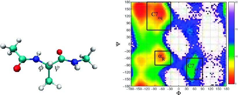
In order to study the numerical behaviors of MSMs and WE methodologies, we first focus on alanine dipeptide. This molecule is usually considered a good model for representing torsional preferences of protein backbones (see Ref. 21 for a related discussion). Its conformation as plotted in Fig. 1 can be displayed on a two dimensional space as a function of torsion angles ϕ and ψ. Fig. 1 provides as well such a representation referred to as the Ramachandran plot of the system, that is its free energy landscape as a function of ψ and ϕ. In this case, the metastable sets $A,B\in {\mathbb{R}}_q^{3\times 22}$ mentioned above correspond to the unfolded and folded states of the protein, which are referred to as C_7eq and C_7ax, respectively. One possible way to define them is represented in Fig. 1: it corresponds to the black squares on the Ramachandran plot.

FIG. 1.

Left: Structure of alanine dipeptide. Right: Ramachandran plot of alanine dipeptide with the unfolded state C_7eq and folded state C_7ax illustrated. Cool colors stand for regions with high free energy.

Although this system is very small, it is an interesting test case, since its free energy landscape is not that simple: the unfolded and folded states are connected by multiple pathways. The numerical experiments were obtained using the molecular dynamics software Gromacs 4.5.3 (see Ref. 22 for further information). The underlying force field ∇V is Amber 96. The temperature is fixed at T = 300 K. The numerical method used to discretize Eq. (1) is the velocity Verlet scheme.

1. Brute force estimation

The reference flux is calculated from a prior database of 100 independent trajectories, that is M = 100. These trajectories, of length T = 100 ns, correspond to independent approximations of one obtained from a velocity Verlet scheme with δt = 2 fs. We calculate mean flux from each trajectory and estimate the standard error as standard deviation of the mean flux times 1.5, which gives 90% confidence interval. The brute force estimation of forward and backward fluxes based on this set of trajectories is

$${\displaystyle {\widehat{\nu }}_R^{A\to B}\approx 0.021\pm 0.003{\mathrm{ns}}^{-1}\text{ and }{\widehat{\nu }}_R^{B\to A}\approx 5.18\pm 0.69{\mathrm{ns}}^{-1},}$$

respectively (corresponding aggregate rate ${\widehat{\nu }}_R=0.021\pm 0.003$).

2. MSMs

All the Markov state models to be considered in this paragraph were built from the 100 MD trajectories that were also used in the brute force estimation. All the trajectories are split into five blocks, each containing 20 trajectories. Five MSMs are built from the blocks. The MSM estimation of flux is equal to the mean of five 1/MFPT, while the error of the estimation is approximated by the standard deviation of the mean times 1.5. We first consider a MSM with a fine partition of the state space that can be represented, in terms of (ϕ, ψ) coordinates, as a regular mesh made of identical squares with size 30° by 30°. Note, we always define C7_eq and C7_ax as single states in any kind of mesh partition in this section. The mesh partition is only for regions out of these two states. It is expected to provide accurate estimation of 1/MFPT. The inverse of forward and backward MFPTs are

$${\displaystyle {\nu }_R^{A\to B}\approx 0.020\pm 0.002{\mathrm{ns}}^{-1}\text{ and }{\nu }_R^{B\to A}\approx 5.10\pm 0.31,}$$

respectively (corresponding aggregate rate ν_R = 0.020 ± 0.002). They match with the brute force estimation very well.

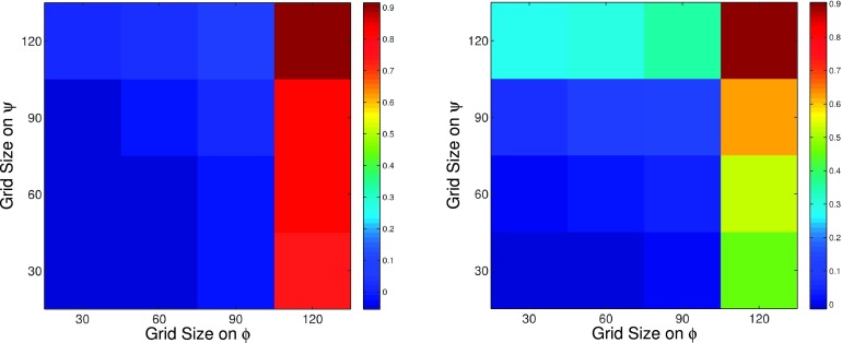
In practice, when dealing with bigger molecules, partitions are much coarser than the ones considered above. Therefore, we want to study the influence of coarseness of partitions on accuracy of MSM estimation of flux. Four grid sizes, 30°, 60°, 90°, and 120°, on ϕ are considered, as well as on ψ axis. There are 16 partitions in total in this experiment, i.e., 30 by 30 and 30 by 60. Fig. 2 shows the relative error of forward and backward flux estimation from 16 MSMs, taking brute force estimation as the reference. Increasing grid size on ϕ worsen accuracy of the flux estimation significantly, while increasing grid size on ψ does not have much effect on the accuracy. We can conclude that the significant transition region for C7_eq to C7_ax transformation is directed along the ϕ axis, particularly through the blue region located at ϕ = 0 and ψ = − 90 in Fig. 1.

FIG. 2.

Relative error of MSM estimation of forward (top) and backward (bottom) fluxes comparing with brute force methodology.

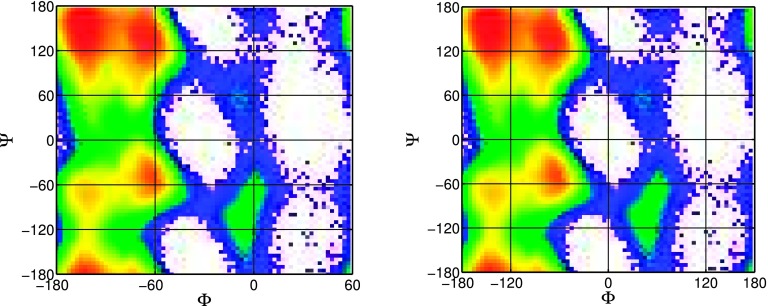
Given that coarse underlying partition leads to biased flux estimation, we further intend to study whether the locations of state boundaries affect accuracy significantly setting the same number of states for underlying partition. As it is shown in Fig. 2, the relative error is significant when grid size on ϕ is increased to 120°. In this experiment, we generate new grid partition by setting grid size ϕ = 120, varying size on ψ, and shifting the original mesh along ϕ axis. Mesh of four sizes is considered, 120° by 30°, 120° by 60°, 120° by 120°, and 120° by 360°. Fig. 3 illustrates the original partition and shifted one (shift is equal to 60°) when the original mesh is 120 by 60.

FIG. 3.

120 by 60 grid partition with shift 0 (top) and shift 60° (bottom).

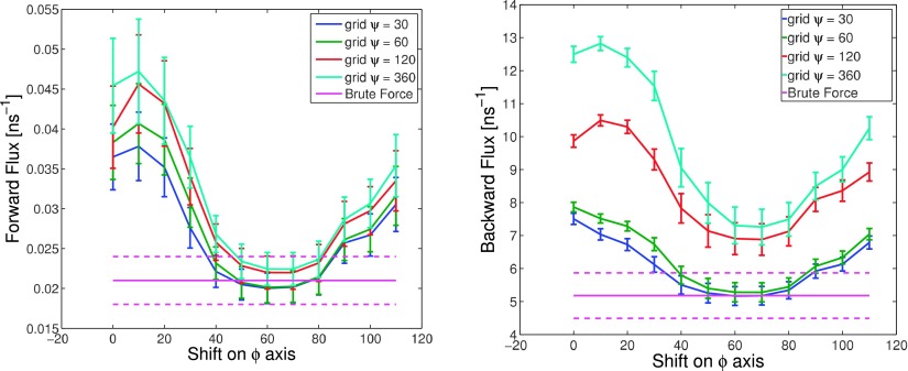
The way the reaction rate depends on the value of the shift in each case has been represented in Fig. 4. This figure clearly illustrates the fact that the resolution of the partition underlying the Markov state model is not the most important factor, since whatever its value, it is possible still to get very close to the reference value. On the contrary, the location of the macro-states boundaries is the crucial point. When the partition is reasonably coarse (thus reflecting a practical situation), the impact of boundary locations is prominent. In order to get accurate rates, one needs to align macro-state boundaries with free energy barriers. Of course, when the mesh size tends to zero, one always obtains accurate values of dynamical quantities. The reason is that, in this case, the boundaries of macro-states are automatically aligned with free energy barriers.

FIG. 4.

Influence of boundaries location. Average estimate forward flux (top) and backward flux (bottom) for reference rectangular partitions with different resolutions, 120° by 30°, 120° by 60°, 120° by 120°, and 120° by 360°, as a function of the shift. The pink line with markers is the reference value.

3. AWE

In this section, we investigate the way changes in the underlying partition impact the performances of AWE, in the same spirit as the study led in Sec. V A 2. The time step involved in the algorithm is δt = 2 fs. The resampling time step is τ₁ = 20 ps. For all partitions, the target number of replicas in each cell is N_C = 30.

We first compute flux from AWE with fine underlining partition, that is a 30° by 30° partition in terms of (ϕ, ψ) coordinates. The C7_eq and C7_ax are still defined as two elements in this partition. Weights of walkers in AWE are initialized according to a MSM that is built from MD trajectories with total length of 2 μs. To match with computational complexity in brute force estimation, here we consider AWE with 368 resamplings (2 μs + 109 cells × 10 walkers × 20 ps × 368 resamplings ≈ 10 μs). The corresponding values of forward and backward fluxes are

$${\displaystyle {\tilde{\nu }}_R^{A\to B}\approx 0.020\pm 0.003{\mathrm{ns}}^{-1}\text{ and }{\tilde{\nu }}_R^{B\to A}\approx 4.7\pm 0.36{\mathrm{ns}}^{-1},}$$

respectively (corresponding aggregate rate ${\tilde{\nu }}_R=0.020\pm 0.003$).

We considered two partitions: 120 by 60 grid and the same grid partition with a 60° shift along the ϕ axis, represented in Fig. 3, with 30 walkers in each cell. In Fig. 5 we have plotted the average forward and backward fluxes estimates corresponding to ${\overline{\phi }}_t=f\left(t\right)$ from 664 iterations of AWE, which matches to 10 μs MD simulations. On each curve, the best estimator of the average reaction rate ${\overline{\phi }}_T$ corresponds to the last point (average of instantaneous fluxes over the whole trajectory). It is then clear that in both cases, the estimate average ${\overline{\phi }}_T$ is close to the reference value ${\hat{\nu }}_R$ (red curve). AWE made significant improvement on accuracy of backward flux estimation, comparing with brute force methodology. Due to resampling, in AWE, same computational resources are used to compute forward and backward fluxes. However, in brute force, most trajectories are working on transitions from unfolded to folded states, which seldom contribute to the computation of backward flux.

FIG. 5.

Average forward ${\overline{\phi }}_n^{A\to B}$ (top) and backward flux ${\overline{\phi }}_n^{B\to A}$ (bottom) estimates as a function of time t = nδt for partitions 120 by 60 grid and 120 by 60 with shift 60 on ϕ axis. The red curve on each plot corresponds to the related average estimator and confidence interval (one standard deviation) computed from brute force simulations.

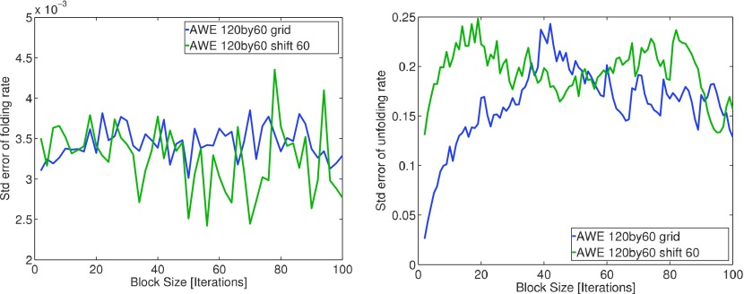
To ensure correct estimation on standard error of AWE flux estimator, Fig. 6 shows convergence of the standard estimates $1.5\cdot \sqrt{{\mathrm{\Sigma }}_{N_b}\left(\phi \left(\omega \right)\right)}$ for both forward and backward fluxes as a function of N_b the number of blocks involved in the block averaging procedure.²⁰

FIG. 6.

Errors of mean forward (top) and backward (bottom) fluxes estimated using block averaging method.²⁰

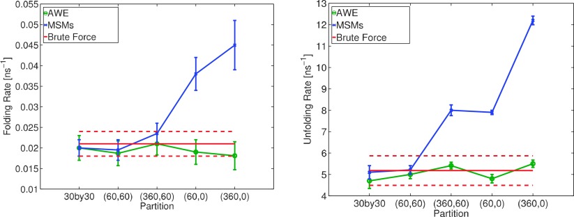
Fig. 7 shows an explicit comparison between MSMs and AWE flux estimators, using five partitions: 30° by 30° grid, 120 by 60 grid with 60° shift on ϕ axis, 120 by 360 grid with 60° shift, 120 by 60 grid with 0° shift, and 120 by 360 with 0° shift. In Appendix B, convergence of flux estimation calculated by AWE using 120 by 360 grid partitions is validated. Fig. 7 explicitly illustrates that AWE provides reliable flux estimation on all partitions, whereas MSMs only provide correct estimation on fine grid partition and the coarse partition with one of the state boundaries located at ϕ = 0. Significant bias occurred using MSMs with 120° by 60° with 0° shift grid partition.

FIG. 7.

Compare AWE with MSM estimations on forward (top) and backward (bottom) fluxes on five different partitions: first partition is 30 by 30 grid and (360, 60) represents grid partition with ϕ = 360 and a shift on ψ axis with 60°.

B. Penta-alanine

Penta-alanine is a more complex biological system comparing to alanine dipeptide. It consists of five alanine residues and 66 atoms. This is the first AWE application based on decomposition of such high dimensional conformational space. All three methodologies, brute force estimation, MSM, and AWE, are based on MD trajectories generated by simulation tool Gromacs4.5.3 using force field Amber96 with implicit solvent. The folding rate under temperature 300 K is studied in this experiment.

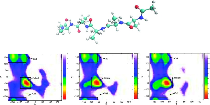
Five alanine residues of penta-alanine construct five ϕ − ψ spaces, and on each of them the distribution of free energy can be visualized. We categorize a conformation to folded or extended state according to the ϕ and ψ angles of the middle three alanine residues (ignore the two alanine residues at terminal). If all three alanine residues are helical, the conformation is considered as folded. On the other hand, if all three alanine residues are coiled, the conformation is categorized to extended. Fig. 8 shows the Ramachandran plots of the middle three alanine residues (ϕ_i, ψ_i)_1≤i≤3, with the helix C_7eq and coil α_R states marked for each residue.

FIG. 8.

Structure of penta-alanine with the middle three ϕ and ψ angles makes as (ϕ_i, ψ_i)_1≤i≤3. Ramachandran plot on the middle three alanine residues. Warmer color represents higher population and lower free energy.

1. Brute force estimation

Five trajectories, each with length 3 μs, time step δt = 2 fs, are generated by MD simulation with general setup introduced in the previous paragraph. Three of them are initialized from extended structure and the other two are initialized from conformations from folded state. From each trajectory, we calculate a folding rate (transition rate from extended to folded state). Mean of the five folding rates is considered as a reference value, which will be used to validate the rate estimation by MSMs and AWE. The 90% confidence interval of brute force estimation is

$${\displaystyle {\widehat{\nu }}_R^{A\to B}\approx (0.033\pm 0.005){\mathrm{ns}}^{-1}.}$$

The relative error is around 15%.

2. MSMs

This section studies performance of MSMs estimation on varying settings of underlying partitions. Since penta-alanine consists of five pairs of ϕ − ψ angles, grid partition on such high dimensional space is infeasible. For example, if we simply decompose each ϕ − ψ space into 4 cells, there will be 4⁵ = 1024 states in total. In fact, only a small subset of this 10 dimensional ϕ − ψ space is accessible by the dynamics of penta-alanine. Therefore, K-centers clustering algorithm²³ implemented in MSMBuilder2.6.0²⁴ is applied to cluster trajectories into K separate states. If sufficient number of states are considered, k-centers clustering algorithm should ensure Markovian property among states. However, it is hard to have sufficient number of states for high dimensional systems.

MSMs are constructed using the five MD trajectories, setting different K’s for clustering. We manually ensure the folded and extended states are defined in a way consistent with Fig. 8 over any k clusterings. Therefore, the folding rates estimation is comparable with brute force method. To estimate statistical error, five MSMs are built, each using single MD trajectory with length 3 μs. 90% confidence interval of flux estimation is computed by 1.5 times the standard deviation of five MSMs flux estimations.

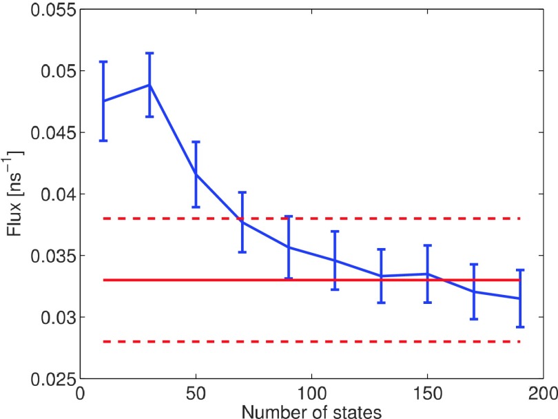
Performance of MSMs model with varying coarseness of underlying partition is studied in this section. Fig. 9 shows the 90% confidence interval of flux (1/MFPT) estimation made by MSM with varying number of states from 10 to 190. Lag time is set to 0.5 ns for all partitions. Appendix C explains the reason why this time lag is chosen for all experiments. The MSM estimation is sensitive to coarseness of underlying partition. With increasing number of states defined, accuracy of MSM improves. MSM with the finest partition (190 states) provides an good flux estimation at

$${\displaystyle {\nu }_R^{A\to B}=0.032\pm 0.002{\mathrm{ns}}^{-1},}$$

FIG. 9.

1/MFPT of penta-alanine estimated by MSM with increasing number of states defined on conformational space.

which falls into the reference interval. Comparing with brute force estimation, the relative error reduces from 15% to 7%. However, with less than 50 states defined, MSM estimation does not fall into the confidence interval of reference flux estimation. Penta-alanine is still a simple system consisting of 66 atoms. However, for a complex biological system consisting of thousands of atoms, defining fine partition on such high dimensional space requires long-term MD trajectories, which introduces a very large computational cost.

3. AWE

In this section, we study the performance of AWE on estimating folding rate of penta-alanine under different coarseness of underlying partitions. AWE consists of two stages: running short MD simulations and resampling. The MD simulation for each walker has the same setup as the experiment of brute force method in Sec. V B 1. Resampling is applied in every 0.5 ns. For the 12 states AWE, 30 walkers are maintained in every state, while 10 walkers are maintained for 102 states AWE.

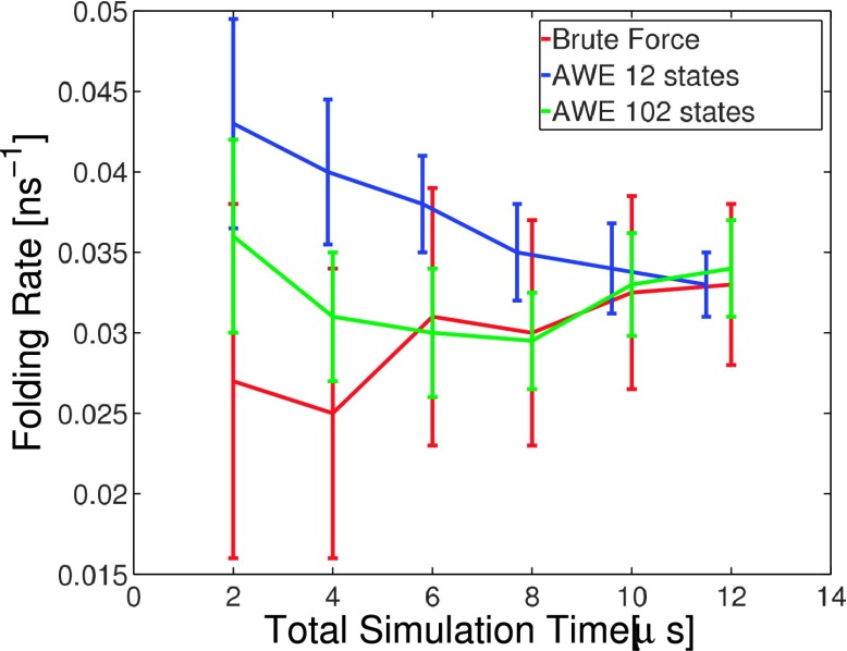
A 3 μs MD trajectory is used for initializing AWE, including running K-centers clustering algorithm to define underlying partition and initializing walkers and their weights according to first eigenvector of the transition matrix built on the MD trajectory. To compare with brute force and MSM, we want to match the total simulation time of AWE to 5 × 3 μs = 15 μs. Here, AWE with two different partitions, 12 states and 102 states, is discussed in detailed convergence and error analysis. For the 12 states partition, 64 iterations of resampling are considered (3 μs + 500 ps × 12 states × 30 walkers × 64resampling ≈ 15 μs). For AWE with 102 states, 24 iterations of resampling is considered (3 μs + 500 ps × 102 states × 10 walkers × 24 resampling ≈ 15 μs). Fig. 10 illustrates convergence of folding rate estimation with increasing total simulation time.

FIG. 10.

AWE folding rate estimation with increasing total simulation time.

The folding rate estimated by 64 iterations AWE sampling with 102 states is

$${\displaystyle {\tilde{\nu }}_R^{A\to B}=(0.034\pm 0.003){\mathrm{ns}}^{-1}.}$$

The folding rate estimation by AWE with 12 states is

$${\displaystyle {\tilde{\nu }}_R^{A\to B}=(0.033\pm 0.002){\mathrm{ns}}^{-1}.}$$

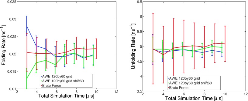
The relative statistical error reduces from 15% to around 6%, comparing to the brute force estimation. Fig. 10 shows that when using varying number of states, AWE estimations always converge to reference interval after certain number of resamplings.

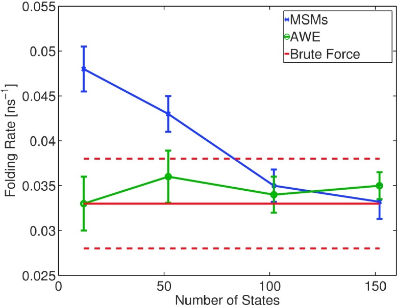
Fig. 11 explicitly compares impact of partition on MSM and AWE flux estimations using four different partitions: 12, 52, 102, and 152 states partitions. Convergence of AWE estimations over total simulation time is included in Appendix B. With more than 102 states defined on conformational space, both MSM and AWE provide an estimation in the reference interval. Using coarser partitions, MSM estimation contains a significant bias, while AWE estimation remains reliable.

FIG. 11.

Compare AWE with MSM built on partitions with different coarseness. X axis indicates number of states defined by k-centers clustering algorithm.

VI. CONCLUSION

In this paper, we have shown through numerical experiments that MSMs are very sensitive to the location of the macro-states that attempt to capture the coarse-grained dynamics. In particular, if the energy barrier along the transition pathway lies “inside” a macro-state, rather than at the boundary, a significant bias is introduced, whereby MSM underestimates the rate. Generally speaking, the bias can be directly related to the height of the barrier within the macro-state that contains it.

One solution, that has been advocated in the MSM literature, is to make the state partition very fine. However, this introduces a very large computational cost and makes it difficult to relate results of the analysis to the macroscopic understanding of the underlying dynamics. Another remedy is to seek to properly align the boundary of the macro-states with important transition regions and saddle points of the free energy. However, in practice, this is difficult to achieve.

On the other hand, AWE, a formulation of weighted ensemble that uses colored walkers to compute fluxes, is much less sensitive to the precise boundaries of coarse-grain dynamics. This suggests that whereas a MSM can provide a good idea of the metastable sets and give a rough estimate of rates, the computation of dynamics quantities may be better done using AWE.

Generally speaking, the AWE method is a strict generalization of MSM in the following sense. Starting at t = 0 with some initial distribution of walkers, we can run one “step” of AWE (that is trajectories of length τ before the first resampling is performed). Then, the rate can be estimated using the transition matrix ${\mathcal{P}}_{ji}$. Up to now, this simulation is in fact strictly identical to a MSM calculation, and therefore the estimate is exactly the same. What AWE is recognizing is that this initial estimate may be biased. If we estimate that the bias is small enough for the purpose at hand, we can stop the simulation here. If not, a resampling is applied and the calculation is continued. Through this process, the distribution of walkers inside the macro-states is progressively relaxed so that, upon convergence, we can recover the “exact” rate with no bias.

So, AWE has really no disadvantage compared to MSM. If we estimate that the bias in MSM is satisfactory, we can stop AWE before the first resampling and get a method identical to MSM. If we decide that the bias is too significant, we apply the full AWE method and get a more accurate estimate after a number of resampling steps.

We would like to point out that several optimizations are possible that were not considered in this paper. (1) The transition matrix can be used to estimate the rates (for the forward, backward, and global relaxation rates) instead of computing the average of the flux. This may provide a more accurate estimate in some cases. (2) The convergence of AWE can be improved by using the equilibrium distribution, as estimated from the transition matrix, to update the macro-state weights (this procedure is distinct from the AWE resampling we are using).

APPENDIX A: INFINITESIMAL GENERATOR OF LANGEVIN DYNAMICS

The infinitesimal generator of process (Q_t, P_t)_t≥0 generated by Langevin dynamics in Eq. (1), denoted by $\mathcal{L}$ and acting on a subset of functions defined on ${\mathbb{R}}_q^{3d}\times {\mathbb{R}}_p^{3d}$ (namely, $D\left(\mathcal{L}\right)$ the domain of $\mathcal{L}$), satisfies

$${\displaystyle \mathcal{L}=-p\cdot {\nabla }_q+M^{-1}\nabla V\cdot {\nabla }_p+M^{-1}\frac{\gamma }{\beta }\left(-{\nabla }_p+M\beta p\right)\cdot {\nabla }_p.}$$

Note that state variable $q=(q_1,\dots ,q_d)\in {\mathbb{R}}_q^{3d}$ is associated to the position process Q, whereas variable $p=(p_1,\dots ,p_d)\in {\mathbb{R}}_p^{3d}$ is associated to the momentum process P. Under appropriate assumptions on V, there exists a probability measure on ${\mathbb{R}}_q^{3d}\times {\mathbb{R}}_p^{3d}$, namely, ψ(t, dq × dp) characterizing the distribution of (Q_t, P_t). It is the solution of the backward Fokker-Planck equation that involves the formal adjoint operator of $\mathcal{L}$, denoted by ${\mathcal{L}}^{\ast }$,

$${\displaystyle \left\{\begin{array}{l}{\partial }_t\psi -p\cdot {\nabla }_q\psi +M^{-1}\nabla V\cdot {\nabla }_p\psi +M^{-1}\frac{\gamma }{\beta }{\nabla }_p\cdot \left({\nabla }_p\psi +M\beta p\psi \right)=0\hfill \\ \psi (0,\cdot )={\mu }_0\hfill \end{array},\right.}$$ (A1)

where μ₀ refers to some arbitrary initial conditions.

Dynamics equation (1) possesses an invariant distribution ρ(dq × dp) such that, if (Q₀, P₀) ∼ ρ, process (Q_t, P_t)_t≥0 is ergodic. Such a measure satisfies ${\mathcal{L}}^{\star }\rho =0$. When μ₀≠ρ, the rate at which the distribution ψ(t, ⋅ ) converges towards ρ is thus related to the spectrum of $\mathcal{L}$. For a rigorous formulation of these statements, see Ref. 25.

APPENDIX B: CONVERGENCE OF AWE EXPERIMENTS

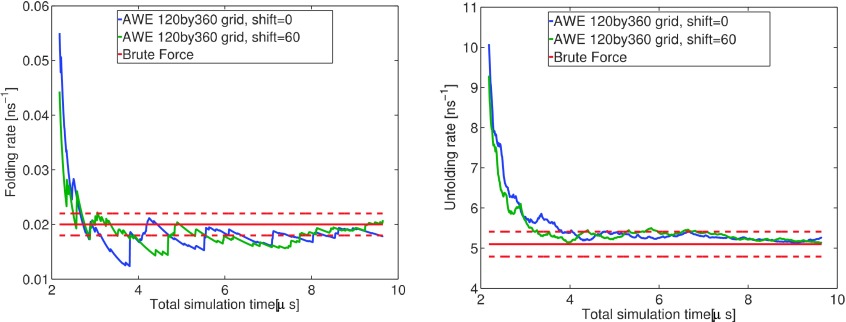
Fig. 12 shows convergence of the average forward flux and backward flux of alanine dipeptide over the total simulation time of AWE on partitions 120 by 360 grid and 120 by 360 with shift 60 on ϕ axis. This validates that the flux shown in Fig. 7 is estimated from converged AWE.

FIG. 12.

Average forward (top) and backward flux (bottom) estimates of alanine dipeptide as a function of time t = nδt for partition 120 by 360 grid and 120 by 360 with shift 60 on ϕ axis. The red lines marked the 90% confidence interval of reference value estimated by brute force methodology.

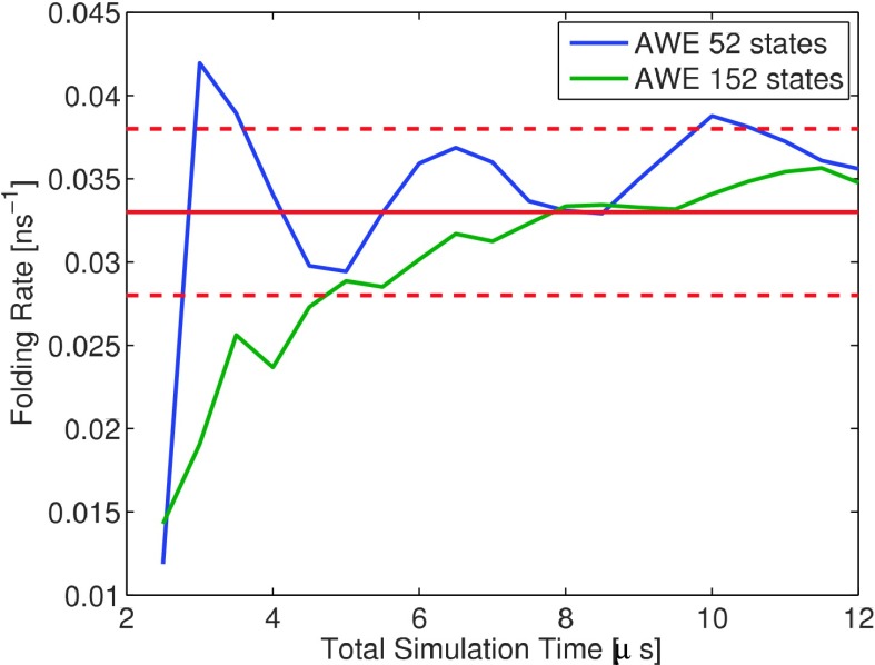
Fig. 13 shows convergence of the average folding rate of penta-alanine over total simulations time, estimated using AWE with 52 and 152 states k-means partitions.

FIG. 13.

Average folding rate estimates of penta-alanine as a function of time t = nδt for 52 and 152 states k-means partitions. The red lines marked the 90% confidence interval of reference value estimated by brute force methodology.

APPENDIX C: IMPLIED TIME SCALES OF PENTA-ALANINE VS. LAG TIME

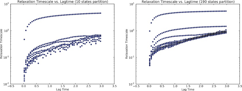
This section shows how to choose right lag time τ for building MSMs for penta-alanine. If a small lag time is chosen, the Markovian property will not be guaranteed, while it leads to bias of MSMs estimation. On the other hand, choosing large lag time leads to significant statistical error of MSMs estimation. Fig. 14 shows the first ten implied time scales of penta-alanine calculated from 10 states MSMs and 190 states MSMs, respectively. We want to choose the earliest point when the implied time scales reach plateau, which is 0.5 ns for both the MSMs models.

FIG. 14.

Implied time scales vs. lag time [ns] of penta-alanine calculated from 10 states MSMs (top) and 190 states MSMs (bottom).

REFERENCES

- 1.Darve E. and Ryu E., “Computing reaction rates in bio-molecular systems using discrete macro-states,” in Innovations in Biomolecular Modeling and Simulations , edited by T. Schlick (RSC Publishing, 2012), Chap. 7, pp. 138–206. 10.1039/9781849735049-00138 [DOI] [Google Scholar]
- 2.Huber G. A. and Kim S., “Weighted ensemble Brownian dynamics simulations for protein association reactions,” Biophys. J. 70, 97–110 (1996). 10.1016/S0006-3495(96)79552-8 [DOI] [PMC free article] [PubMed] [Google Scholar]
- 3.Bhatt D. and Zuckerman D. M., “Heterogeneous path ensembles for conformational transitions in semiatomistic models of adenylate kinase,” J. Chem. Theory Comput. 6, 3527–3539 (2010). 10.1021/ct100406t [DOI] [PMC free article] [PubMed] [Google Scholar]
- 4.Bhatt D., Zhang B. W., and Zuckerman D. M., “Steady-state simulations using weighted ensemble path sampling,” J. Chem. Phys. 133, 014110 (2010). 10.1063/1.3456985 [DOI] [PMC free article] [PubMed] [Google Scholar]
- 5.Suarez E. and Zuckerman D. M., “Learning from history: Non-Markovian analyses of complex trajectories for extracting long-time behavior,” Biophys. J. 108, 160a (2015). 10.1016/j.bpj.2014.11.883 [DOI] [Google Scholar]
- 6.Singhal N. and Pande V. S., “Error analysis and efficient sampling in markovian state models for molecular dynamics,” J. Chem. Phys. 123, 204909 (2005). 10.1063/1.2116947 [DOI] [PubMed] [Google Scholar]
- 7.Swope W. C., Pitera J. W., and Suits F., “Describing protein folding kinetics by molecular dynamics simulations. 1. Theory,” J. Phys. Chem. B 108, 6571–6581 (2004). 10.1021/jp037421y [DOI] [Google Scholar]
- 8.Pande V. S., Beauchamp K., and Bowman G. R., “Everything you wanted to know about Markov state models but were afraid to ask,” Methods 52, 99–105 (2010). 10.1016/j.ymeth.2010.06.002 [DOI] [PMC free article] [PubMed] [Google Scholar]
- 9.Metzner P., Schütte C., and Vanden-Eijnden E., “Transition path theory for Markov jump processes,” Multiscale Model. Simul. 7, 1192–1219 (2009). 10.1137/070699500 [DOI] [Google Scholar]
- 10.Prinz J.-H., Chodera J. D., Pande V. S., Swope W. D., Smith J. C., and Noé F., “Optimal use of data in parallel tempering simulations for the construction of discrete-state Markov models of biomolecular dynamics,” J. Chem. Phys. 134, 244108 (2011). 10.1063/1.3592153 [DOI] [PMC free article] [PubMed] [Google Scholar]
- 11.Sarich M., Noé F., and Schütte C., “On the approximation quality of markov state models,” Multiscale Model. Simul. 8, 1154–1177 (2010). 10.1137/090764049 [DOI] [Google Scholar]
- 12.Djurdjevac N., Sarich M., and Schütte C., “Estimating the eigenvalue error of Markov state models,” Multiscale Model. Simul. 10, 61–81 (2012). 10.1137/100798910 [DOI] [Google Scholar]
- 13.Zhang B. W., Jasnow D., and Zuckerman D. M., “Efficient and verified simulation of a path ensemble for conformational change in a united-residue model of calmodulin,” Proc. Natl. Acad. Sci. U. S. A. 104, 18043–18048 (2007). 10.1073/pnas.0706349104 [DOI] [PMC free article] [PubMed] [Google Scholar]
- 14.Zhang B. W., Jasnow D., and Zuckerman D. M., “Weighted ensemble path sampling for multiple reaction channels” (2009); e-print arXiv:0902.2772v1 [physics.bio-ph].
- 15.Zhang B. W., Jasnow D., and Zuckerman D. M., “The ‘weighted ensemble’ path sampling method is statistically exact for a broad class of stochastic processes and binning procedures,” J. Chem. Phys. 132, 054107 (2010). 10.1063/1.3306345 [DOI] [PMC free article] [PubMed] [Google Scholar]
- 16.Bhatt D. and Zuckerman D. M., “Symmetry of forward and reverse path populations” (2010), e-print arXiv:1002.2402v2 [physics.comp-ph].
- 17.Costaouec R., Feng H., Izaguirre J., and Darve E., “Analysis of the accelerated weighted ensemble methodology,” Discrete and Continuous Dynamical Systems (2013), pp. 171–181. [Google Scholar]
- 18.Abdul-Wahid B., Feng H., Rajan D., Costaouec R., Darve E., Thain D., and Izaguirre J. A., “AWE-WQ: Fast-forwarding molecular dynamics using the accelerated weighted ensemble,” J. Chem. Inf. Model. 54, 3033–3043 (2014). 10.1021/ci500321g [DOI] [PMC free article] [PubMed] [Google Scholar]
- 19.E W. and Vanden-Eijnden E., “Towards a theory of transition paths,” J. Stat. Phys. 123, 503–523 (2006). 10.1007/s10955-005-9003-9 [DOI] [Google Scholar]
- 20.Flyvbjerg H. and Petersen H. G., “Error estimates on averages of correlated data,” J. Chem. Phys. 91, 461 (1989). 10.1063/1.457480 [DOI] [Google Scholar]
- 21.Feig M., “Is alanine dipeptide a good model for representing the torsional preferences of protein backbones,” J. Chem. Theory Comput. 4, 1555–1564 (2008). 10.1021/ct800153n [DOI] [PubMed] [Google Scholar]
- 22.Hess B., Kutzner C., Van Der Spoel D., and Lindahl E., “Gromacs 4: Algorithms for highly efficient, load-balanced, and scalable molecular simulation,” J. Chem. Theory Comput. 4, 435–447 (2008). 10.1021/ct700301q [DOI] [PubMed] [Google Scholar]
- 23.Bowman G. R. and Pande V. S., “Using generalized ensemble simulations and Markov state models to identify conformational states,” Methods 49, 197–201 (2009). 10.1016/j.ymeth.2009.04.013 [DOI] [PMC free article] [PubMed] [Google Scholar]
- 24.Beauchamp K. A., Bowman G. R., Lane T. J., Maibaum L., Haque I. S., and Pande V. S., “Msmbuilder2: Modeling conformational dynamics at the picosecond to millisecond timescale,” J. Chem. Theory Comput. 7, 3412–3419 (2011). 10.1021/ct200463m [DOI] [PMC free article] [PubMed] [Google Scholar]
- 25.Hellfner B. and Nier F., “Hypoelliptic estimates and spectral theory for Fokker–Planck operators and witten Laplacians,” in Lecture Notes in Mathematics (Springer, 2005). [Google Scholar]