Magnetic Moment Quantifications of Small Spherical Objects in MRI

Abstract

Purpose

The purpose of this work is to develop a method for accurately quantifying effective magnetic moments of spherical-like small objects from magnetic resonance imaging (MRI). A standard 3D gradient echo sequence with only one echo time is intended for our approach to measure the effective magnetic moment of a given object of interest.

Methods

Our method sums over complex MR signals around the object and equates those sums to equations derived from the magnetostatic theory. With those equations, our method is able to determine the center of the object with subpixel precision. By rewriting those equations, the effective magnetic moment of the object becomes the only unknown to be solved. Each quantified effective magnetic moment has an uncertainty that is derived from the error propagation method. If the volume of the object can be measured from spin echo images, the susceptibility difference between the object and its surrounding can be further quantified from the effective magnetic moment. Numerical simulations, a variety of glass beads in phantom studies with different MR imaging parameters from a 1.5 T machine, and measurements from a SQUID (superconducting quantum interference device) based magnetometer have been conducted to test the robustness of our method.

Results

Quantified effective magnetic moments and susceptibility differences from different imaging parameters and methods all agree with each other within two standard deviations of estimated uncertainties.

Conclusion

An MRI method is developed to accurately quantify the effective magnetic moment of a given small object of interest. Most results are accurate within 10% of true values and roughly half of the total results are accurate within 5% of true values using very reasonable imaging parameters. Our method is minimally affected by the partial volume, dephasing, and phase aliasing effects. Our next goal is to apply this method to in vivo studies.

1 Introduction

Cerebral microbleeds and small calcifications appear as small dark round spots in magnetic resonance (MR) magnitude images. They exist in elder populations or patients with dementia (e.g., see [1]). Currently, except for number counting, there is no effective method of quantifying these objects. Similarly, localized nanoparticles also appear as dark round spots in images (e.g., see [2]). The least squares fit method is currently the “best” method of quantifying magnetic moments of nanoparticles [2]. However, a good fit to the magnetic field distribution requires many voxels outside the nanoparticle dephasing region. As the magnetic field outside an object decreases quickly, the least squares fit method is only useful for an object with a very large magnetic moment. When the magnetic moment of an object is not large enough, even in the 2D case, the least squares fit method becomes inaccurate [3]. Recent quantitative susceptibility mapping (QSM) techniques also cannot accurately measure the magnetic moments or susceptibilities of small objects (e.g., see [4]). In fact, before one can reliably quantify susceptibility of a small object from MRI, one must first quantify the magnetic moment of the object. This is particularly true if we only use MR phase images to quantify the magnetic property of a spherical object, as phase is proportional to the effective magnetic moment of the object rather than the susceptibility alone. This makes the quantification of magnetic moment as important as the quantification of susceptibility for small objects in MRI.

In this paper, we demonstrate a new method in the quantification of effective magnetic moments of spheres from MR images. This 3D method follows similar ideas described in the 2D case [5] but its mathematical derivations are much more complicated. The combination of this 3D method and the previous 2D cylindrical method is the CISSCO (Complex Image Summation around a Spherical or a Cylindrical Object) method. The CISSCO method relies only on the known imaging parameters and assumes that an object of interest is a sphere or an infinitely long cylinder. From the magnetostatic theory [6], in the first order approximation, the magnetic moment of a small object with an arbitrary geometry is equal to that of a perfect sphere. This concept makes our 3D method described in this paper applicable to spherical-like objects such as microbleeds, nanoparticles, and maybe industrial particles [7].

In the following sections, a procedure and its mathematical proof will be given to identify the center of the spherical object. Detailed procedures of magnetic moment quantification will be presented. Uncertainties of quantified magnetic moments including both the thermal noise from the object of interest and the systematic errors due to discrete pixels will be studied from the error propagation method [8]. By minimizing the uncertainty due to the thermal noise, we will derive the criteria of how to effectively evaluate the magnetic moment of a given object in images. Effective magnetic moments of glass beads will be measured by both MRI and a SQUID (superconducting quantum interference device) based magnetometer. Results of simulations and phantom studies from different imaging parameters will be compared and will be followed by discussions. Although we focus on objects without MR signals in this paper, the procedures of measuring the magnetic moment are applicable to objects with signals (see Eq. (1) and Eq. (6) below).

2 Methods

The basic concept of the CISSCO method is to add the complex MR signal of each voxel around an object of interest. From the statement in the above introduction, this object can be modeled as a perfect sphere. The overall signal from space within a concentric sphere of the spherical object is given by [9]

$$S={\rho }_0{\int }_0^{2\pi }d\varphi {\int }_0^{\pi }d\theta \text{sin}\theta {\int }_a^R{\mathit{drr}}^2{e}^{-ip(3{cos}^2\theta -1)/r^3}+s_c=\frac{4\pi }{9\sqrt{3}}{\rho }_0{a}^3{\int }_{-1}^2\mathit{dxD}(x)e^{-\mathit{igx}}+s_c$$ (1)

where p ≡ γΔχB₀T_Ea³/3 and D(x) is proportional to the density-of-states

$$\begin{array}{cccc}D(x)& =& \frac{1}{x^2}(2-x)\sqrt{1+x}& \mathit{when}x\in (-1,-\lambda )or(2\lambda ,2)\\ & =& \frac{1}{x^2}\left[(2-x)\sqrt{1+x}-\left(2-\frac{x}{\lambda }\right)\sqrt{1+\frac{x}{\lambda }}\right]& \mathit{when}x\in (-\lambda ,2\lambda )\\ & =& 0& \mathit{otherwise}\end{array}$$ (2)

The effective spin density of the material outside the spherical object is modeled as a constant ρ₀, which depends on imaging and tissue parameters such as relaxation times. The signal from the spherical object itself is s_c and is a constant (real number) depending on object volume and imaging parameters. The radius of the object is a. The effective magnetic moment p (hereafter magnetic moment, unless otherwise specified) is defined as ga³ and the extremum phase g is defined as γΔχB₀T_E/3, where γ is the gyromagnetic ratio 2π·42.58 MHz/T, Δχ is the magnetic susceptibility difference between the susceptibility of the object and that of the surrounding material, B₀ is the MRI main field strength, and T_E is the echo time. Hereafter the word susceptibility refers to Δχ unless otherwise specified, as this is the variable that MRI measures. The azimuthal angle θ is measured from the main field direction and is defined by the spherical coordinate. The distance r is measured from the center of the object in the spherical coordinate. Lastly, λ ≡ (a/R)³ is the volume fraction where R is the user defined radius of a concentric sphere. If the center of the object can be determined and thus the concentric sphere can be correctly positioned, the unknowns in Eq. (1) to be solved are ρ₀, Δχ, a, and s_c.

In principle, the theoretical signal S can be compared to the actual signal and those unknowns may be quantified. However, as there are various types of noise to consider and the center of the spherical object must also be determined, the biggest challenge is to identify a set of robust procedures for accurate quantification of the magnetic moment which is directly related to the susceptibility.

2.1 Numerical simulations

We conduct three sets of simulations. The first task is to validate Eq. (1) with numerical simulations. We assign zero signal inside each spherical object but unity for ρ₀ in this first study. The radius of a simulated spherical object (a) has to be at least 32 grid points in order to reduce the error within 0.3%, due to an imperfect spherical surface. The main field B₀ and the echo time T_E are chosen to 1.5 T and 5 ms, respectively. The susceptibility difference Δχ is changed from 10^{− 3} ppm to 10⁴ ppm by every order of magnitude. The overall signal S within a given radius R can be calculated by replacing the 3D integrals in Eq. (1) by the discrete sums of the complex signal at each grid point. On the other hand, the complex signal S can also be calculated directly from the single integral, using Eq. (2). If Eq. (1) is correct, both results should be equal to each other. Several values of R are used in our simulations. For Δχ ≤ 1 ppm, the value of R is chosen to be at least 6 grid points larger than the radius a, in order to have sufficient signals included in S. For Δχ > 1 ppm, the radius R varies but it should satisfy 0.1 ≤ p/R³ ≤ π. (See Section 3.3 for the reason of limiting p/R³ in this range.) The comparisons between the discrete sums and integrals of signals from Eq. (1) provide us the numerical errors in our method.

The purpose of the second set of simulations is to properly model the discrete nature of MRI data. This will allow us to study the systematic noise (or error) due to discrete voxels in MRI. For this purpose, we simulate MR signals induced from a sphere with a fixed radius of 32 points on 1024³ grid points in the spatial domain but at different echo times. Then we Fourier transform the simulated data into k-space based on the definition used in MRI (e.g., see [10]), take the central 32³ points in k-space, and inverse Fourier transform the data back to the spatial domain. These processes mimic the digitized (or discretized) MR signal and the reconstructed MR images, which display a spherical object with an effective radius of one pixel and a field-of-view of 32 pixels. With a limited computer memory, we first need to simulate and perform Fourier transformation of every 1024² points, store the data in the hard drive, and then repeat the process through the third dimension. Other parameters used in simulations are B₀= 1.5 T, ρ₀= 10 units, and Δχ = 10 ppm. Echo times 5 ms, 10 ms, 15 ms, and 20 ms are used in this set of simulations. We also shift the centers of spherical objects in our simulations and study the effects. For example, if we shift the center of an object by 8 points on the original 1024³ grid, we effectively shift the object center by 0.25 pixel on the reconstructed 32³ images.

The systematic noise (ε in Eq. (15) below) is calculated as the absolute difference between the real part of the simulated signal (within a given R) and that of the theoretical signal (from the integral of Eq. (1) with Eq. (2)) divided by the real part of the theoretical signal. The object centers at different subpixel positions, g, and a are also inputs to our simulations in order to calculate systematic errors.

The purpose of the third set of simulations aims to add the thermal noise onto the above second set of images. The thermal noise is Gaussian distributed with a zero mean and a standard deviation σ. The thermal noise is added onto the real and imaginary part of the images and is generated by a random number generator [11]. The theoretical signal to noise ratio (SNR) in images is defined by ρ₀/σ. In our simulated images, we choose an SNR of 10:1. This is achieved by assigning one unit to the standard deviation in the Gaussian distributions (as ρ₀= 10 units). Example images without and with a shifted object center are shown in Fig. 1.

Figure 1.

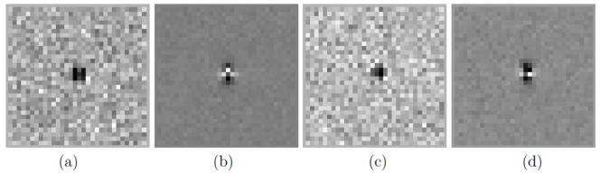
Examples of simulated images. Coronal views are displayed here. The SNR is 10:1 and echo time is 5 ms in these images. Radius of the object is 1 pixel. Other parameters used in simulations are described in the text. (a) Magnitude and (b) its associated phase image of a spherical object whose center is located at the corner of a voxel. In this case, the center of the object is considered as unshifted. (c) Magnitude and (d) its associated phase image of the same object whose center, however, has been shifted by roughly 0.3 pixel along both the x -direction and the z -direction. Thus, the overall shift of the object center is roughly 0.42 pixel. The phase pattern right around the object in (d) is clearly different from that in (b).

Most of our simulations were performed on a personal computer with an Intel Pentium 4 Processor of 2.6 GHz and 2.56 GB memory. Some tests were carried out in higher power computers. Although Mathematica, Matlab, C, and C++ programs were used in simulations and following calculations, the C and C++ programs were the major utilities.

2.2 Calculations of signals from images

In order to improve the accuracy when adding MR signals from images within a sphere of a given radius R, we have divided each voxel into 1000 subvoxels (i.e., a factor of 10 along each direction). The MR signal in each subvoxel is 0.001 of the signal in the original voxel. This procedure is applied throughout this paper whenever the overall complex signal within a radius R is calculated from either simulated or phantom images.

2.3 Identifying the center of a spherical object

Equation (1) is valid only when the center of the spherical object is identical to the center of the concentric sphere with a radius R. Thus before the quantification of the magnetic moment, we need to identify the center of the object. We have considered three possible procedures. One is to maximize the real part of the signal from a given spherical shell around the object. Another is to minimize the real part of the signal within a given sphere. The other is to identify the object center at which the sum of the phase values of the complex signals within a given sphere is zero (given the (3cos²θ − 1)/r³ phase distributions). The main idea in each procedure is to choose a sphere or a shell, move the sphere or shell around the object, sum up the complex signals or phases within the sphere or shell, and determine the object center when the minimal or maximal value of the overall summed signals has occurred. Equivalently, in the following proofs, we consider a fixed shell and a fixed sphere with their centers at the origin, but move the spherical object around. When extremum occurs, the center of the object will coincide with the center of the fixed shell or the center of the fixed sphere.

In the procedure of maximizing the real part of the shell signal, the object should be completely inside the inner sphere of the shell. Assume that the shell is formed by two concentric spheres with radii R₁ and R₂ and a < R₂ <R₁. The center of the object is assumed to be located at coordinates (x₀, y₀, z₀) with $\sqrt{x_0^2+y_0^2+z_0^2}+a\equiv r_0+a\le R_2$. The MR signal from the shell is

$$S={\rho }_0{\int }_{R_2}^{R_1}{\mathit{drr}}^2{\int }_0^{2\pi }d\varphi {\int }_0^{\pi }d\theta \text{sin}\theta exp\left\{-i\frac{p}{d^3}(3{cos}^2{\theta }^{\prime }-1)\right\}$$ (3)

where d² = (rcosϕ sinθ − x₀)²+ (rsinϕ sinθ − y₀)²+ (rcosθ − z₀)² and d cosθ′+ z₀= r cosθ. One can analytically derive that, at r₀ = 0, $\frac{\partial S}{\partial x_0}=\frac{\partial S}{\partial y_0}=\frac{\partial S}{\partial z_0}=0$. Derivations of second derivatives are provided in Appendix 7.

The second approach is to minimize the real part of the signal within one sphere with a radius R. With the parameters defined above and with r₀< a, the MR signal of the concentric sphere is

$$S={\rho }_0{\int }_0^{2\pi }d\varphi {\int }_0^{\pi }d\theta \text{sin}\theta {\int }_{{\rho }^{\prime }(\theta ,\varphi )}^R{\mathit{drr}}^{2}exp\left\{-i\frac{p}{d^3}(3{cos}^2{\theta }^{\prime }-1)\right\}+s_c$$ (4)

where ρ′(θ, ϕ) satisfies (ρ′ cosϕ sinθ − x₀)² + (ρ′ sinϕ sinθ − y₀)²+ (ρ′ cosθ − z₀)² = a² and

$${\rho }^{\prime }(\theta ,\varphi )=x_{0}cos\varphi sin\theta +y_{0}sin\varphi sin\theta +z_{0}cos\theta +\sqrt{{(x_{0}cos\varphi sin\theta +y_{0}sin\varphi sin\theta +z_{0}cos\theta )}^2+(a^2-x_0^2-y_0^2-z_0^2)}$$ (5)

It is obvious that at r₀= 0, ρ′(θ,ϕ) = a. Again, one can analytically prove that, at r₀= 0, $\frac{\partial S}{\partial x_0}=\frac{\partial S}{\partial y_0}=\frac{\partial S}{\partial z_0}=0$. Derivations of second derivatives are shown in Appendix 8. How the radius R is chosen is further described in the Results section.

2.4 Quantification of the effective magnetic moment

The 3D integral form in Eq. (1) implies that the summed MR signal from an arbitrary shell depends only on the moment p and spin density ρ₀. If we choose a shell formed by two concentric spheres with radii R₁> R₂, then the MR signal of the shell is S₁ − S₂, which satisfies

$$\frac{9\sqrt{3}}{4\pi {\rho }_0}(S_1-S_2)=R_1^3{\int }_1^{R_1^3/R_2^3}\frac{dx}{x^2}(2e^{\mathit{ixp}/R_1^3}+e^{-2\mathit{ixp}/R_1^3})+{\int }_{-1}^2\frac{dx}{x^2}[2-(2-x)\sqrt{1-x}](R_1^3{e}^{-\mathit{ixp}/R_1^3}-R_2^3{e}^{-\mathit{ixp}/R_2^3})$$ (6)

where S₁ and S₂ are the MR complex signals calculated from their corresponding radii R₁ and R₂. In order to derive Eq. (6), the following identity is used so no singularity is created in the integrands.

$${\int }_{-\lambda }^{2\lambda }\frac{dx}{x^2}\left[(2-x)\sqrt{1+x}-\left(2-\frac{x}{\lambda }\right)\sqrt{1+\frac{x}{\lambda }}\right]e^{-\mathit{igx}}={\int }_{-\lambda }^{2\lambda }\frac{dx}{x^2}\left[(2-x)\sqrt{1+x}-2\right]e^{-\mathit{igx}}+{\int }_{-\lambda }^{2\lambda }\frac{dx}{x^2}\left[2-\left(2-\frac{x}{\lambda }\right)\sqrt{1+\frac{x}{\lambda }}\right]e^{-\mathit{igx}}$$ (7)

In theory, Eq. (6) itself seems sufficient to solve the two unknowns (p and ρ₀) from a complex shell signal. However, our experience reveals that a calculation utilizing only the imaginary part of Eq. (6) can lead to an inaccurate determination of the effective magnetic moment. This may be due to a lack of the first order imaginary term when one expands Eq. (6) into a Taylor series in p. Thus we use three concentric spheres to quantify the magnetic moment. Assume that the radii of the three arbitrary spheres satisfy R₁> R₂> R₃. Their corresponding MR complex signals are S₁, S₂, and S₃. We can solve the magnitude of p from

$$Re(S_1-S_2)Re(f_{23})-Re(S_2-S_3)Re(f_{12})=0$$ (8)

where we define Re(f_ij) as

$$Re(f_{ij})\equiv Re\left(\frac{9\sqrt{3}}{4\pi {\rho }_0}(S_i-S_j)\right)\mathit{with}i,j=1,2,3$$ (9)

and where S_is appearing in Eq. (8) are the complex signals directly taken from images, but Eq. ?? is calculated using the theoretical formula in Eq. (6) or its alikeness. The magnetic moment p is the only unknown in Eq. (8). Since we only use the real parts in Eq. (8) to solve the magnetic moment, we can only determine |p|. After that, we can compare the imaginary part of S₁ − S₂ (or S₂ − S₃) to the right hand side of Eq. (6) but with p replaced by |p|. If the imaginary part of the signal is above the thermal noise (depending on the choices of R_is) and if the Gibbs ringing effect due to the object can be neglected, this comparison can determine the sign of p.

The optimal choices of the three radii will be determined when the uncertainty of p is minimized and discussed in the next subsection. This can be done by rewriting Re(f_ij)

$$Re(f_{ij})=\frac{p}{{\varphi }_i}{\int }_1^{{\varphi }_j/{\varphi }_i}\frac{dx}{x^2}[2cos(x{\varphi }_i)+cos(2x{\varphi }_i)]+{\int }_{-1}^2\frac{dx}{x^2}[2-(2-x)\sqrt{1+x}]\left[\frac{p}{{\varphi }_i}cos(x{\varphi }_i)-\frac{p}{{\varphi }_j}cos(x{\varphi }_j)\right]$$ (10)

where we define ϕ_i as

$${\varphi }_i\equiv p/R_i^3\mathit{with}i=1,2,3$$ (11)

As each ϕ_i turns out to be a phase value on the equatorial plane of the object (see the argument in the exponential function on the left hand side of Eq. (1)), a choice of R_i leads to a rough estimation of p. In order to avoid the dephasing and the phase aliasing effect, we can choose R₃ sufficiently large such that $\mid p\mid /R_3^3$ is less than π. On the other hand, we want to keep R₁ small enough such that ρ₀ within the radius R₁ is approximately a constant. These two considerations indicate that |p| is between 0 and $\pi R_3^3$. The Van Wijngaarden-Dekker-Brent method [11] can be used to numerically solve |p|. The mean value theorem of integral calculus refers to that the root of a function is unique in a given range when the derivative of the function is not zero in that entire range. As the derivative of Eq. (8) with respect to p is the denominator D in Eq. (12) in uncertainty calculations, for a meaningful result of p between 0 and $\pi R_3^3$, the value of D cannot be zero. Thus the solution of | p | from Eq. (8) is unique.

2.5 Uncertainties of the effective magnetic moment

As described earlier, the inevitable sources of uncertainties and errors are from the thermal noise and systematic noise. These two noise sources are uncorrelated. We can analytically formulate the overall uncertainty from Eq. (8) through the error propagation method [8]. The basic concept is to calculate the first derivative of the real part of Eq. (6) and its counter part of Re(S₂ − S₃). The uncertainty of p, δp, in percentage is

$$\frac{\delta p}{\mid p\mid }=\frac{1}{\mid D\mid }\sqrt{{(\delta [Re(S_2-S_3)])}^2\frac{{(Re(f_{12}))}^2}{p^2}+{(\delta [Re(S_1-S_2)])}^2\frac{{(Re(f_{23}))}^2}{p^2}}$$ (12)

where

$$D=Re(S_1-S_2)Re\frac{\partial f_{23}}{\partial p}-Re(S_2-S_3)Re\frac{\partial f_{12}}{\partial p}$$ (13)

$$Re\frac{\partial f_{ij}}{\partial p}=-2{\int }_1^{{\varphi }_j/{\varphi }_i}\frac{dx}{x}[sin(x{\varphi }_i)+sin(2x{\varphi }_i)]+{\int }_{-1}^2\frac{dx}{x}[2-(2-x)\sqrt{1+x}][sin(x{\varphi }_j)-sin(x{\varphi }_i)]$$ (14)

In the above derivation, we have assumed no correlation between S₁ − S₂ and S₂ − S₃. Their variances are

$${(\delta [Re(S_i-S_j)])}^2={[{\epsilon }_{ij}Re(S_i-S_j)]}^2+\frac{4\pi }{3}{\sigma }^2(R_i^3-R_j^3)\mathrm{\Delta }x\mathrm{\Delta }y\mathrm{\Delta }z$$ (15)

where ε_ij is the systematic error in percentage and is calculated by neglecting the thermal noise (i.e., infinite SNR). The voxel volume is ΔxΔyΔz. If the systematic noise can be neglected, Eq. (12) is proportional to $\sqrt{\mathrm{\Delta }x\mathrm{\Delta }y\mathrm{\Delta }z}/(\mathrm{S}NR\sqrt{\mid p\mid })$ and the rest only depends on ϕ_i defined in Eq. (11). As we have limited each ϕ_i between 0 and π, for any given image resolution, SNR, and the effective magnetic moment of the object, we can numerically determine the minimal value of δp/|p| in Eq. (12) by varying ϕ_i. The optimal combination of (ϕ₁, ϕ₂, ϕ₃) provides a guidance of how to choose radii of the three concentric spheres. Due to discrete voxels, precise values of radii are not required in our approach. In our estimation of the uncertainty, we have assumed that the center of the object is correctly identified, even though this is not completely true.

2.6 Resolving the magnetic susceptibility and volume of the object individually

One way to determine susceptibility (or g) is to measure the volume of the object from spin echo images and then calculate Δχ (or g) from the magnetic moment, as g = p/a³. However, this approach is valid only when the object has no spin density (s_c = 0) and if the dephasing effect due to Δχ through sampling in the spin echo images can be neglected. The latter condition may be satisfied by increasing the image resolution, but at the expense of SNR and imaging time. Consider the real part of the MR signal S_SE from an arbitrarily uniform volume V that encloses the entire object on spin echo images

$$S_{SE}={\rho }_{0,SE}(V-V_0)\equiv {\rho }_{0,SE}\left(V-\frac{4\pi }{3}{a}^3\right)$$ (16)

where ρ_0,SE is the effective spin density (a constant) around the object in the spin echo images. With two arbitrary volumes V₁ and V₂ such that V₂ is completely enclosed by V₁, ρ_0,SE and the volume of the object V₀ = 4πa³/3 can be determined from

$$\begin{array}{l}{S}_{1,SE}={\rho }_{0,SE}(V_1-V_0)={\rho }_{0,SE}(V_1-V_2)+{\rho }_{0,SE}(V_2-V_0)\\ S_{2,SE}={\rho }_{0,SE}(V_2-V_0)\end{array}$$ (17)

which leads to

$$V_0=(S_{1,SE}{V}_2-S_{2,SE}{V}_1)/(S_{1,SE}-S_{2,SE})$$ (18)

As the signals S_1,SE − S_2,SE and S_2,SE are uncorrelated and their thermal noises are proportional to the square root of number of voxels, the uncertainty of the object volume can be derived from the error propagation method [8]

$$\delta V_0=\frac{\sqrt{\mathrm{\Delta }v}}{\mathrm{S}{NR}_{SE}}\sqrt{V_2+\frac{{(V_2-V_0)}^2}{V_1-V_2}}$$ (19)

where Δv is the voxel volume of the spin echo images and SNR_SE is the SNR in the spin echo images. In order to minimize the uncertainty, it is obvious that the volume V₁ − V₂ should be chosen as large as possible before heterogeneity is encountered in the images, while the volume V₂ should be chosen as small as possible but still larger than the object. In fact, in order to estimate the volume of the object more accurately, V₂ has to be larger than the volume covering both the distorted object and voxels due to its shifted image intensity in the spin echo image. In our analyses, for simplicity, we have used the magnitude part of the spin echo images rather than the real part.

2.7 Phantom studies

We prepared three gel phantoms with different sizes of spherical glass beads and imaged them with a 1.5 T MR machine (Siemens Sonata) at different echo times for the validation of our method. We measured the diameter of each glass bead ten times with a vernier caliper. We mixed 107 g of gelatin powders into 1200 ml distilled water for each phantom. After placing a glass bead on the top of a solidified gel layer in a container, we poured more gelatin solution into the container. This process was repeated until two or three beads were embedded in each gel phantom. The first phantom contained two glass beads of diameters 3 mm and 5 mm and a hollow straw (see Fig. 2). The straw served as a reference such that the absolute magnetic susceptibility of the gel was validated as that of water, −9.05 ppm in SI units [5]. Coronal images of a multiple echo 3D gradient echo sequence and of a 3D turbo spin echo sequence were acquired. The imaging parameters of the gradient echo sequence for the first phantom were T_E = 5 ms, 10 ms, 15 ms, and 20 ms, T_R = 25 ms, flip angle 15°, resolution 1 mm × 1 mm × 1 mm, field of views 256 mm × 256 mm × 96 mm, and read bandwidth 610 Hz per pixel (Hz/pixel) for T_E = 5 ms and 220 Hz/pixel for the other three echo times. The scan time for the gradient echo sequence was 615 sec. Imaging parameters of the 3D spin echo sequence were T_E = 71 ms, T_R = 600 ms, flip angle of the refocusing pulse 160°, turbo factor 25, resolution 1 mm × 1 mm × 1 mm, field of views 256 mm × 256 mm × 96 mm, read bandwidths 610 Hz/pixel, actual phase encoding lines 275, actual partition encoding steps 112, and the scan time was 740 sec for this spin echo sequence.

Figure 2.

(a) The magnitude and (b) its associated phase image show a 5 mm glass bead in the coronal view acquired at echo time 10 ms from a 1.5 T MR machine. (c) The magnitude image and (d) its associated phase image show a 3 mm glass bead (pointed by the white arrow) and the cross session of an air straw. The 1.5 T MRI machine adopts the right-handed convention. Note the somewhat opposite phase patterns outside the bead and the air straw. The main field direction is along the up-down direction of each image.

The second phantom contained two beads of diameters 2 mm and 6 mm. The parameters of the gradient echo sequence for the second phantom were identical to the above parameters, except that the number of slices was 72 and the read bandwidth was 350 Hz/pixel for all four echoes. The use of different read bandwidths was to test whether this imaging parameter would affect our quantitative method. A circular polarized radiofrequency (rf) head coil was used to image the first two phantoms.

In order to study the effect of the magnetic moment measurement due to heterogeneous image intensity, we placed another set of 2 mm, 3 mm, and 5 mm beads in the third gel phantom and imaged the phantom with an 8-channel rf coil. Imaging parameters of the 3D gradient echo sequence were mostly the same as those stated above, except that the number of slices was 64, the read bandwidth was 350 Hz/pixel for all four echoes, and two averages were used for this scan. We acquired both the combined magnitude images (using the sum-of-squares method for reconstruction) and original k-space data from each channel. The magnetic moments quantified from single channel k-space data were compared with the moments obtained from the combined magnitude images but with phase images from single channels.

To remove the background field in phase images, we first chose a volume-of-interest (VOI) within the phantom and around each bead. Manual phase unwrapping followed by a 3D second order polynomial fitting were performed within each VOI. The dimension of a VOI along each independent direction was about 3–4 times of the diameter of the bead. In addition, each VOI also excluded certain voxels nearby each bead, as those voxels contained measurable phase information from the bead itself. After the fit, we subtracted the polynomial from the original phase images and thus removed the unwanted background field around each bead.

2.8 Magnetic moment measurements by SQUID

Absolute magnetic moments of the 2 mm, 3 mm, 5 mm, and 6 mm glass beads from the first two phantoms were also measured with a SQUID based magnetometer (Quantum Design MPMS-5S), at fields between 0.5 T and 5.0 T in intervals of 0.5 T. At each field strength, the magnetic moment of each bead was measured 10 times and the averaged value and standard deviation of the magnetic moment were obtained. The measurements at 1.5 T were compared to results derived from our CISSCO method.

Except for the 2 mm glass bead, each bead was placed inside a straw that was mounted to the magnetometer for measurements. The 2 mm bead was placed inside a capsule and then was fixed inside the straw by a cotton ball. The magnetic moments of the experimental setups without beads were also measured and were subtracted from the measurements with beads. After the absolute magnetic moment of each bead was measured, the absolute susceptibility was calculated from the magnetic moment divided by 1.5 T and by the volume of each bead (V_0′ in Table 4). We compare the susceptibility values between SQUID and MRI.

Table 4.

The volume estimations of glass beads imaged by a spin echo sequence. The first column lists the diameters of glass beads measured by a vernier caliper. The second column lists the pseudo volume V₁. The third column lists the pseudo volume V₂. The fourth column shows the estimated volume V₀ from spin echo images. The fifth column is the calculated volume based on the first column. The sixth column is the difference in percentage between V₀ and V_0′. Accurate volume measurements of beads without MR signal can be obtained from spin echo images.

Diameters of	V1	V2	V0	V0′	Diff
glass beads (mm)	(mm3)	(mm3)	(mm3)	(mm3)	%
2.06 ± 0.05	320	57	4.4 ± 0.3	4.6 ± 0.3	4.3
3.08 ± 0.02	440	63	15.2 ± 0.3	15.3 ± 0.3	0.6
5.03 ± 0.10	1536	199	67.3 ± 0.4	66.6 ± 4.0	1.0
6.02 ± 0.10	1678	378	109.0 ± 0.8	114.2 ± 5.7	4.5

3 Results

3.1 Numerical simulations

In general, the numerical errors from simulations are small. The numerical error of the real part of the complex signal in Eq. (1) is no more than 0.3%, while the numerical error of the imaginary part of the complex signal in Eq. (1) is between 0.2% to 0.3%. These results indicate that under infinite image resolution, our theoretical derivations agree well with numerical calculations.

After the proper reconstruction of 32³ images with different small spherical objects, without adding the thermal noise, for most cases, we have found that the real part of the total complex signal from either a sphere or a shell is within 3% of the theoretical value given by Eq. (1) or Eq. (6). However, the imaginary part of the total signal or phase can deviate from the theoretical value by 100%. Such a large error is due to the point spread function of the object or due to the lack of the first order term of the magnetic moment. As long as the real part is used in the quantification of the magnetic moment, such a large error due to the imaginary part or phase of the signal does not seem to lead to any inaccurate quantification.

3.2 Identification of the object center

Among the three possible procedures of identifying the object center, we have found that the sole use of the imaginary part of the MR signal does not lead to an accurate determination. As a result, the phase approach fails. For the procedure of using a shell to determine the object center, the second derivatives of the real part of the signal S with respect to all directions have to be negative. However, from numerical evaluations of the equations provided in Appendix 7, this will occur only when ϕ₁ and ϕ₂ are certain values. This result suggests that using a shell is not a robust procedure to determine the center of the object. We also confirm that from our simulations.

The best procedure of identifying the object center is to use the one sphere approach. When the real part of the signal is minimized by moving the sphere around the object, the object center is determined. In this approach, the second derivatives of the real part of the signal S with respect to all three directions have to be positive. From numerical evaluations of the equations in Appendix 8, these conditions can be satisfied when ϕ_R is less than roughly 2.1 radians. On the other hand, the radius R should not be chosen larger than a radius whose ϕ_R is less than 0.1 radian, as such a choice can lead to insensitive results of second derivatives. We suggest to choose a radius R with the corresponding ϕ_R between 1 and 2 radians, if possible. As a rough value of ϕ_R can be estimated from certain pixels on the equatorial plane in phase images, the magnetic moment p can also be estimated from ϕ_RR³. With the one sphere approach and the implementation of a downhill simplex program from [11], it typically takes our Pentium 4 roughly 20 seconds to identify the center of an object with p < 30 radian · pixel³.

From our numerical simulations, the identified center of each object is within 0.3 voxel of the actual center, whether the thermal noise has been added into the images or not. A 0.3 voxel deviation away from the actual center is relatively large and it occurs when centers of objects have been purposely shifted by 0.4 voxel in either or all three directions. However, even in those situations, the quantified magnetic moments of the objects are still accurate (i.e., within the uncertainties estimated by Eq. (12)).

3.3 Measurements of the magnetic moment: simulation results

We first want to determine the three optimal radii used for the quantification of the magnetic moment. This can be found by minimizing the uncertainty of the magnetic moment in Eq. (12). By neglecting the systematic errors ε_ij, we have found that (ϕ₃, ϕ₂, ϕ₁) are best in the range of (π −2.6, 1.0–0.7, ≤ 0.1) radians. A choice of R₂ with a corresponding phase value of ϕ₂ ≈ 0.9 radian would provide a slightly lower uncertainty. Given these phase ranges and Eq. (11), R₁ may be chosen as roughly 3R₃. Similarly, R₂ may be chosen as roughly 1.4R₃ or 0.5R₁. None of these three radii needs to be a multiple integer of a pixel. The ranges of ϕ_is also imply that R₁ can be chosen as large as possible but should not be too large to include significant phase values from any nearby objects. The radius R₃ can be chosen as small as possible but larger than phase aliasing areas around the object. We typically choose the three radii within these ranges of ϕ_i values. However, in order to reduce systematic errors due to the Gibbs ringing effects, our studies show that it is better to choose R₃ at least half a pixel away from the surface of the object. In addition, the difference between each R_i is better to be at least one pixel. These two rules of choosing radii for moment measurements supersede the above selection rules. We follow all these rules and list results in Tables 1 and 2. Nonetheless, if these two rules are used, particularly for objects with small magnetic moments or phase values, it is obvious that the above simple relations between the three radii for minimizing uncertainty due to the thermal noise may not be met.

Table 1.

Magnetic moments quantified from simulated images at four different echo times with and without simulated thermal noise. The first column lists the echo time. The second column lists three radii used in Eq. (8) to solve p. The third column lists their corresponding phase values directly measured from images. These values are different from $p/R_i^3$, as explained in the text. The fourth column lists p_ideal ≡ γΔχB₀T_Ea³/3. The fifth and seventh column list quantified p values. The sixth and eighth column list the uncertainty of p calculated from Eq. (12). The uncertainty in the sixth column only includes the discrete error, but that in the eighth column includes both thermal and discrete noise. All quantified magnetic moments except for one agree with ideal values within 5% of the ideal values. The differences between quantified values and ideal values are properly covered by the uncertainties calculated from Eq. (12).

TE	radii	phase	pideal	w/o thermal noise		w/ thermal noise
(ms)	(pixel)	(radian)	(rad · pixel 3)	p	δp/p (%)	p	δp/p (%)
	(1.5, 2.5, 3.5)	(1.56, 0.58, 0.16)	6.69	7.11	5.5	6.81	6.0
	(1.8, 2.8, 4.0)	(2.42, 1.26, 0.20)	13.4	13.5	2.5	13.4	3.2
	(2.1, 3.1, 5.0)	(1.78, 0.64, 0.16)	20.1	20.4	1.8	20.3	2.5
	(2.4, 3.4, 5.0)	(2.23, 0.89, 0.22)	26.8	26.9	1.1	26.8	2.0

Table 2.

Magnetic moments of glass beads 2 mm, 3 mm, 5 mm and 6 mm at four different echo times were measured by the CISSCO method. The first column lists the echo time. The second and seventh column list the values of three radii (in units of mm or pixel) used in Eq. (8) to solve for each magnetic moment. The third and eighth column list quantified magnetic moments. The fourth and ninth column show the uncertainties of magnetic moments (in percentage). The uncertainties are calculated from Eq. (12), including both thermal noise and systematic noise. The fifth, sixth, tenth, and eleventh column list uncertainties of systematic noise calculated from simulations. The SNR of the images at four different echo times is about 13:1. Quantified magnetic moments per echo time for each bead agree with each other within two standard deviations of the uncertainties, except for the 6 mm bead measured at T_E = 5 ms. Half of the overall estimated uncertainties are no more than 5%.

	Diameter 2 mm					Diameter 3 mm
TE	radii	p	δ	ε12	ε23	radii	p	δ	ε12	ε23
(ms)	(mm)	(rad · mm 3)	(%)			(mm)	(rad · mm 3)	(%)
	(1.5, 2.5, 3.5)	− 1.28	45	0.001	0.010	(2.0, 3.0, 4.0)	−5.54	15	0.004	0.014
	(1.5, 2.5, 3.5)	− 3.05	21	0.001	0.026	(2.0, 3.0, 4.0)	−10.45	11	0.005	0.040
	(1.5, 2.5, 3.5)	− 4.90	13	0.001	0.040	(2.0, 3.0, 4.0)	−14.71	6	0.008	0.040
	(1.5, 2.5, 3.5)	− 6.48	7	0.001	0.034	(2.0, 3.0, 4.5)	−18.24	2	0.005	0.019
(a)

	Diameter 5 mm					Diameter 6 mm
TE	radii	p	δ	ε12	ε23	radii	p	δ	ε12	ε23
(ms)	(mm)	(rad · mm 3)	(%)			(mm)	(rad · mm 3)	(%)
	(3.0, 4.0, 5.0)	−20.93	8	0.003	0.013	(3.5, 4.5, 6.0)	−26.39	3	0.003	0.001
	(3.0, 4.0, 5.8)	−40.41	5	0.004	0.033	(3.5, 4.5, 6.7)	−62.67	2	0.004	0.015
	(3.0, 4.2, 6.7)	−57.94	1	0.004	0.008	(3.5, 4.7, 7.7)	−92.16	1	0.001	0.015
	(3.1, 4.4, 7.4)	−76.05	1	0.003	0.014	(3.5, 5.0, 8.6)	−127.00	1	0.002	0.032
(b)

Quantified magnetic moments of simulated objects at four different echo times with and without thermal noise added into images are shown in Table 1. The listed phase values (third column) in Table 1 are measured from the equatorial plane of each object at their corresponding radii (second column). Due to discretized MR voxels and averaged MR complex signal within each voxel, a phase value measured from each voxel may not agree with the actual phase value (p/R³). As given by the theory, the measured magnetic moments appear to be proportional to the echo time T_E. In all eight cases, the maximal uncertainty (one standard deviation) of the measurement is no more than 6% of the actual magnetic moment. The difference between the measured magnetic moment and the actual moment for any case (except for one) is less than the uncertainty calculated from Eq. (12).

3.4 Measurements of the magnetic moment: phantom results

Table 2 lists the quantified magnetic moments of four glass beads at four different echo times. Most uncertainties calculated from Eq. (12) are less than 20%. Even though in most cases the effective magnetic moments of glass beads are larger than those values used in simulations, as ϕ₃ in most cases are not close to the ideal value, the uncertainties in Table 2 are usually larger than those shown in Table 1. While the exact magnetic moment of each glass bead is not known in advance, Table 2 has shown that the magnetic moment of each bead is proportional to the echo time (and independent of the read bandwidth) within estimated uncertainties. However, one exception occurs for the 6 mm bead at T_E = 5 and 20 ms. Our further investigations have ruled out most possibilities and hence suggested that at T_E = 5 ms, poor eddy current compensations result in residual unwanted phase in the original phase images. At T_E = 20 ms, as the phase induced from the bead extends to the largest area, residual background phase from the phantom itself has made some influences. In both cases, the second order polynomial fit did not seem to completely remove the unwanted background phase in images.

Results from the 8-channel coil are shown in Table 3. As the magnitude intensity around the background of each bead does not vary too much, the results from the combined channel for each bead also agree with the results from the single channel. The SNR used in Eq. (12) can take into account intensity variations in magnitude images and, in the worst case, the SNR can be chosen as 1:1. The results from the 8-channel coil are also consistent with those shown in Table 2, but we notice that for the 5 mm bead, the magnetic moments in Table 3 are roughly 9% lower than those listed in Table 2. Measuring the diameter of the second bead (used in the third phantom), we find a diameter of 4.98±0.04 mm. While this value is still consistent with the diameter shown in Table 4, this slight reduction of the diameter leads to a 3% reduction in volume and thus in the magnetic moment measurements. The remaining 6% differences between the two sets of measurements could be due to the susceptibility difference between the two 5 mm beads, or due to the lack of quality assurance checks on the clinical MR machine, since the third phantom was scanned several months behind the first two phantoms.

Table 3.

Magnetic moments of glass beads 2 mm, 3 mm, and 5 mm at four different echo times quantified from combined 8-channel images and from single channel images. For single channel data, we use images reconstructed from k-space from one of the 8 channels. For combined data, we use the same phase images as those from the single channel, but for the magnitude part we use the multichannel (sum of squares) data. The first column lists the echo time. The second, sixth, and tenth column are quantified magnetic moments from the combined data. The fourth, eighth, and twelve column are the measured magnetic moments from the single channel data. The column following each quantified magnetic moment lists its associated uncertainty, which includes both thermal noise and systematic noise calculated from Eq. (12). The SNR of images at all four echo times is about 15:1. Quantified magnetic moments per echo time for each bead again agree with each other within two standard deviations of the uncertainties. Measurements between two different coils for each bead also have good agreements.

	Diameter 2 mm				Diameter 3 mm				Diameter 5 mm
TE	pSS	δp/p	pch	δp/p	pSS	δp/p	pch	δp/p	pSS	δp/p	pch	δp/p
(ms)	(rad · mm3)	(%)	(rad · mm3)	(%)	(rad · mm3)	(%)	(rad · mm3)	(%)	(rad · mm3)	(%)	(rad · mm3)	(%)
	1.69	35	1.85	29	4.80	26	5.04	24	18.92	13	19.20	13
	3.90	17	4.17	15	9.76	17	9.72	17	37.48	8	37.35	8
	5.42	14	5.47	14	14.59	8	14.70	8	53.74	1	53.89	1
	7.00	8	7.05	8	18.44	2	18.51	2	70.49	1	70.30	1

3.5 Estimations of object volumes

When an object such as a glass bead produces no signal in MRI, the volume of the object and its uncertainty can be calculated from spin echo images, based on Eq. (18) and Eq. (19). With an SNR of 30:1 in the spin echo images, the measured volumes and associated uncertainties are shown in Table 4. Table 4 also lists the mean diameter and its associated standard deviation of each glass bead measured from a vernier scale. The difference between the volume measured from spin echo images and that from the vernier scale is within 5% for any glass bead.

3.6 SQUID measurements

The results from SQUID measurements in general agree with those from the CISSCO method. The absolute magnetic moments averaged from 10 SQUID measurements at 1.5 T are (−6.09±0.062) *10⁻⁸ A·m ², (−1.97±0.0087) *10⁻⁷ A·m ², (−8.06±0.27) *10⁻⁷ A·m ², and (−1.52±0.00068) *10⁻⁶ A·m ², for the 2 mm, 3 mm, 5 mm, and 6 mm bead, respectively. The absolute susceptibility of each glass bead is calculated from the absolute magnetic moment and is listed in Table 5. Although the standard deviations of these magnetic moments are small or negligible, the actual uncertainties from SQUID measurements are large. For example, when the same beads were measured by SQUID on a different day, the measured magnetic moments were roughly 16%, 17%, 6%, and 16% deviated from the above values for the 2 mm, 3 mm, 5 mm, and 6 mm bead, respectively. These deviations are likely due to environmental background noise caused by nearby electrical circuits that is difficult to shield. In addition, the magnetic moment of the capsule and cotton ball is roughly 9 times of the magnetic moment of the 2 mm bead. These facts imply that the actual error of SQUID measurements is probably about 3*10⁻⁸ A·m ². The 16% difference from the 6 mm bead may be due to whether the glass bead was mounted slightly off the center of the magnetometer, as the bead was considered as an oversized object for our SQUID-based magnetometer.

Table 5.

Comparisons of magnetic susceptibility measurements between MRI and SQUID. The first column lists the diameters of glass beads. The second column lists calculated susceptibilities (Δχ) from magnetic moments of glass beads obtained at T_E =15 ms in Table 2 and from volumes V_0′ in Table 4. The uncertainties of susceptibility values were calculated through the error propagation method. These are results from MRI. The third column lists the absolute susceptibility value of each bead, by adding −9.05 ppm (which is the absolute susceptibility of water) to each value shown in the second column. We assume no uncertainty of the water susceptibility value. The fourth column lists measured susceptibility of each bead from SQUID. Measurements between our CISSCO method from MRI and SQUID agree within uncertainties. However, different sizes of beads seem to have slightly different susceptibility values.

Beads	MRI	MRI + water	SQUID
2 mm	−2.23 ± 0.32 ppm	−11.3 ± 0.3 ppm	−11.1 ± 0.7 ppm
3 mm	−2.01 ± 0.13 ppm	−11.1 ± 0.1 ppm	−10.8 ± 0.2 ppm
5 mm	−1.82 ± 0.11 ppm	−10.9 ± 0.1 ppm	−10.1 ± 0.7 ppm
6 mm	−1.68 ± 0.09 ppm	−10.7 ± 0.1 ppm	−11.2 ± 0.6 ppm

In order to compare SQUID results to MR results, we need to add the absolute susceptibility of water, χ_H2O =−9.05 ppm, to the susceptibility values measured from MRI. This is because the susceptibility from MRI, Δχ, is defined as χ_gb − χ_H2O, where χ_gb is the absolute susceptibility of the glass bead. The calculated absolute susceptibility values of glass beads from MRI are also listed in Table 5. They agree with those measurements from SQUID within uncertainties.

4 Discussion

Our simulations and phantom studies have demonstrated that the CISSCO method can accurately quantify magnetic moments of small objects. The word “small” is measured relatively to an image resolution on a particular MRI machine. For this reason and for fair comparison of results from different machines with different sequence parameters, it is better to use radian · pixel ³ as the unit for CISSCO measurements. In the following subsections, we will discuss certain issues related to the measurements of magnetic moments, susceptibility quantifications, and the background phase removal methods.

4.1 Quantifications of magnetic moments

4.1.1 Choices of the three radii

For a small object with a high susceptibility value (or a long echo time or a high field strength), the CISSCO method can reliably quantify a magnetic moment down to a few radian · pixel ³, as indicated in Table 1. On the other hand, for a relatively large object with a small susceptibility value (or a short echo time or a low field strength), the quantified magnetic moment can have a large uncertainty. First, we note that the choices of three concentric spheres with radii R_i will always lead to a solution from Eq. (8). However, due to insufficient phase information around the object of interest, R_is may not be optimal values given at the beginning of Sec. 3.3 (when only the thermal noise is considered). Furthermore, in order to reduce any significant systematic errors due to discrete image pixels, R₃ (the smallest radius of choice) should be at least half a pixel away from the surface of the object and the radius between each R_i needs to be differed by one pixel. The larger the R_i is, the smaller the systematic error is. The choices of non-optimal R_is can lead to a larger uncertainty of the measured magnetic moment, due to the presence of the thermal noise. Some of such results can be seen in Table 2. Generally speaking, given the optimal ranges of R_is in Sec. 3.3, the phase value at the equatorial plane on the surface of the object (i.e., | g |≡| p |/a³) is better to be at least 3 radians in order to obtain accurate results. This can be challenging for MRI studies if Δχ is too small.

4.1.2 Determination of the sign of a quantified magnetic moment

The phase term, − p(3cos²θ−1)/r³, shown in Eq. (1) has a minus sign and this left-handed definition follows the convention in [10]. On the other hand, many MRI vendors (including ours) use the right-handed definition [12], which leads to a sign change in the phase term. As a result, quantified magnetic moment or susceptibility can also have a sign change. Thus, one should be careful about interpreting measurements from MR images and determine whether an object of interest is paramagnetic or diamagnetic to water. As an example, Fig. 2d shows phase distributions from a glass bead and from an air straw (in a cylindrical shape). As the glass bead is diamagnetic to water but air is paramagnetic to water, we see somewhat opposite phase patterns around those two objects. (Note that the air straw has a cos 2ψ phase distributions outside the straw, as it is a 2D object.)

One may think to determine the magnetism of an object by visually examining phase intensities appearing in images. This can be dangerous, as Fig. 1b and Fig. 1d clearly show different phase intensities and patterns of the same object, especially for phase values inside the object. A reliable way is to quantify the imaginary part of the sum from the CISSCO method, as describe in the above text.

4.1.3 No major effect due to a slightly shifted center of the object

Solving the magnetic moment from Eq. (8) takes no more than one second of the computer time. However, as stated above, it can take 20 seconds or longer on a Pentium 4 to determine the center of an object. In addition, the identified center may not be the actual center, due to the presence of noise in images. This can happen when phase values around the object are close to zero. As a result, the sum of the complex signal does not differ much using either the identified center or one of its neighboring subpixels. Visual inspections of the object centers are needed in those situations. As long as the identified center of the object is close to the true center, the quantified magnetic moment is also very close to its true value.

4.1.4 Comparisons between CISSCO and other methods

Due to discrete voxels, the phase outside the object of interest does not exactly follow the 1/r³ decay. This is the main reason why the least squares fit is not able to accurately determine the magnetic moment of a small object. The CISSCO method avoids this problem by summing up MR signals of neighboring voxels. For comparison, the magnetic moments measured by Bos et al. [2] using the least squares fit range from roughly 21.6 radian · pixel ³ to 359 radian · pixel ³. Those moments are sufficiently large and can be accurately quantified by CISSCO. For another comparison, recent work by Liu et al. [4] shows that mean magnetic moments of glass beads have been underestimated by at least 10%, using a susceptibility mapping method. Their mean magnetic moments of air bubbles were even much worse. On the other hand, we accidentally discover a small air bubble in images of the third phantom. The quantified volume of that air bubble is a little bit under 1 mm ³ and thus its uncertainty is over 20%. However, with this volume, the quantified susceptibility is about −9.26 ppm, compared to the ideal −9.4 ppm.

4.2 Susceptibility quantifications

4.2.1 Different beads showing slightly different susceptibility values

As the 3D second order polynomial fit may not effectively remove the background phase at the longest echo time for the 6 mm bead, which has widest phase distributions, we use results from T_E =15 ms shown in Table 2 for the estimations of susceptibility values listed in Table 5. We are surprised that susceptibility values from different beads are slightly different, although those values still agree with each other within two standard deviations of the uncertainty. Perhaps those differences are realistic, due to possibly small contaminations during manufacturing processes, as we could imagine that different beads were made from different dewar or machines. Nonetheless, comparing the results of two different 5 mm beads shown in Table 2 and Table 3, and given the susceptibility results from Table 5, these results suggest that the CISSCO method has the accuracy to distinguish small changes between quantified magnetic moments.

4.2.2 A reason why the susceptibility cannot be solved from Eq. (1)

After solving the magnetic moment p, one may think to use Eq. (1) to further solve the susceptibility of the object, when s_c = 0. Unfortunately this is not realistic, as explained here. With the help of Eq. (7), we can rewrite Eq. (1) to be

$$\frac{9\sqrt{3}}{4\pi {\rho }_0{R}^3}S=2{\int }_1^{1/\lambda }\frac{dx}{x^2}{e}^{i\lambda gx}+{\int }_1^{1/\lambda }\frac{dx}{x^2}{e}^{-i2\lambda gx}+{\int }_{-1}^2\frac{dx}{x^2}\left[2-(2-x)\sqrt{1+x}\right]e^{-i\lambda gx}+\lambda {\int }_{-1}^2\frac{dx}{x^2}\left[(2-x)\sqrt{1+x}-2\right]e^{-\mathit{igx}}$$ (20)

Note that λg ≡ p/R³ and radius R is at our choice. If we consider a known p and a fixed R, but consider λ→0 (and thus g→∞), Eq. (20) clearly shows that the signal S quickly approaches to an asymptotic value. With the presence of noise in MR systems, this derivation suggests that Eq. (1) can only allow us to determine an upper bound of the object volume and thus the lower bound of the susceptibility (or g). For example, when a nanoparticle is smaller than an imaging voxel, we may accurately determine its magnetic moment with our CISSCO method, but are not able to determine its volume from Eq. (1).

4.3 Background phase removal methods

4.3.1 Problems of different methods

In this work, we use a 3D second order polynomial fit method to remove the background phase in phantom images. While such a polynomial fit is not perfect, at least it will not overcorrect phase values induced from glass beads. We have also tried to use a 32×32 high pass filter to remove the background field. When magnetic moments of beads are not large, the results from the high pass filter are about the same as those shown in Table 2. However, when a magnetic moment is larger than 70 radian · pixel ³, such a high pass filter size will significantly reduce the quantified result. If we reduce the size of the high pass filter to, say, 16×16, such a high pass filter size cannot effectively remove the background phase distributions induced from the geometry of the phantom container at long echo times. Thus, for a uniform presentation of the scientific work here, we have chosen the polynomial fit over the high pass filter. A recent SHARP (Sophisticated Harmonic Artifact Reduction for Phase) method [13] is also not suitable for us, as the theory behind that method requires only a spherical surface, but the method sums up phase values within a spherical volume. If the volume has included an object or has cut through an object, then the theory is violated. In addition, the spherical kernel used in SHARP should be large enough in order to mimic a perfect sphere. However, such a choice will remove pixels close to the boundary of the phantom container but we need those pixels for phase induced from beads at long echo times.

4.3.2 Future work

In reality, even if we can completely remove the unwanted background field, an object of interest can still be affected by the magnetic field produced from a nearby tissue. If we can approximate that field as a local uniform field around the object, then the absolute value of Eq. (6) may be used to solve p. The procedure of identifying the object center will need to be modified as well. These should be considered before the CISSCO method can be applied to in vivo images. On the other hand, a constant background phase globally appearing in a uniform phantom can be usually removed by a high pass filter, which does not appear to alter the susceptibility of a small object [3].

5 Conclusion

We have developed and demonstrated that the CISSCO method can accurately quantify magnetic moments of several small objects from standard 3D gradient echo MR images. Our method has three advantages. First, we can reliably quantify the effective magnetic moment as low as a few radian · pixel ³. This means that the radius of the object can be much smaller than a pixel. Second, the uncertainty of each measurement from CISSCO is reduced by summing up voxels around the object. The uncertainty can be further reduced if the echo time can be increased without losing SNR. Third, as a result, the quantified magnetic moment or susceptibility of the object can be accurate within 10% and sometimes within 5% of the true value for practical applications and within reasonable imaging time. We have demonstrated those results with simulations and phantom studies. Our next goal is to apply the CISSCO method to in vivo small objects such as microbleeds in the brain or nanoparticles labeling cells.

Appendix

A Maximizing the real part of the signal from a spherical shell to identify the object center

In order to calculate the derivatives of signal S in Eq. (3), we first calculate the derivatives of its integrand. We define

$$f\equiv e^{ip(3{cos}^2{\theta }^{\prime }-1)/d^3}$$ (21)

and we obtain

$$\begin{array}{l}\frac{\partial f}{\partial x_0}=-\frac{3\mathit{ipf}}{d^7}[4{(rcos\theta -z_0)}^2-{(rsin\theta cos\varphi -x_0)}^2-{(rsin\theta sin\varphi -y_0)}^2](rsin\theta cos\varphi -x_0)\\ \frac{\partial f}{\partial y_0}=-\frac{3\mathit{ipf}}{d^7}[4{(rcos\theta -z_0)}^2-{(rsin\theta cos\varphi -x_0)}^2-{(rsin\theta sin\varphi -y_0)}^2](rsin\theta sin\varphi -y_0)\\ \frac{\partial f}{\partial z_0}=-\frac{3\mathit{ipf}}{d^7}[3{(rsin\theta cos\varphi -x_0)}^2+3{(rsin\theta sin\varphi -y_0)}^2-2{(rcos\theta -z_0)}^2](z_0-rcos\theta )\end{array}$$ (22)

We can easily find that the first derivatives and the cross terms of the second derivatives of S are all zero at r₀ = 0. The remaining second derivatives at r₀ = 0 are

$$\begin{array}{l}{\frac{{\partial }^{2}S}{\partial x_0^2}|}_{r_0=0}=-6\pi p{\rho }_0\left[3p{\int }_{R_2}^{R_1}\frac{dr}{r^6}{\int }_0^{1}dx{(5x^2-1)}^2(1-x^2)f_0-i{\int }_{R_2}^{R_1}\frac{dr}{r^3}{\int }_0^{1}dx(35x^4-30x^2+3)f_0\right]\\ {\frac{{\partial }^{2}S}{\partial y_0^2}|}_{r_0=0}={\frac{{\partial }^{2}S}{\partial x_0^2}|}_{r_0=0}\\ {\frac{{\partial }^{2}S}{\partial z_0^2}|}_{r_0=0}=-12\pi p{\rho }_0\left[3p{\int }_{R_2}^{R_1}\frac{dr}{r^6}{\int }_0^{1}dx{(3-5x^2)}^2{x}^2{f}_0+i{\int }_{R_2}^{R_1}\frac{dr}{r^3}{\int }_0^{1}dx(35x^4-30x^2+3)f_0\right]\end{array}$$ (23)

where f₀ ≡ e^{−ip(3x2−1)/r3}. By changing the variable r to ϕ and defining ϕ ≡ p/r³, ${\varphi }_1\equiv p/R_1^3$, and ${\varphi }_2\equiv p/R_2^3$, we can rewrite the above equations to

$$\begin{array}{l}{\frac{{\partial }^{2}S}{\partial x_0^2}|}_{r_0=0}=-2\pi p^{1/3}{\rho }_0\left[3{\int }_{{\varphi }_1}^{{\varphi }_2}{\varphi }^{2/3}d\varphi {\int }_0^{1}dx{(5x^2-1)}^2(1-x^2)f_{\varphi }-i{\int }_{{\varphi }_1}^{{\varphi }_2}\frac{d\varphi }{{\varphi }^{1/3}}{\int }_0^{1}dx(35x^4-30x^2+3)f_{\varphi }\right]\\ {\frac{{\partial }^{2}S}{\partial z_0^2}|}_{r_0=0}=-4\pi p^{1/3}{\rho }_0\left[3{\int }_{{\varphi }_1}^{{\varphi }_2}{\varphi }^{2/3}d\varphi {\int }_0^{1}dx{(3-5x^2)}^2{x}^2{f}_{\varphi }+i{\int }_{{\varphi }_1}^{{\varphi }_2}\frac{d\varphi }{{\varphi }^{1/3}}{\int }_0^{1}dx(35x^4-30x^2+3)f_{\varphi }\right]\end{array}$$ (24)

where f_ϕ ≡ exp{−iϕ(3x² − 1)}. Only the real part of the above equations are invariant when p is changed to −p. Thus, we only use the real part to identify the object center.

B Minimizing the real part of the signal within a sphere to identify the object center

Following the derivation in the above Appendix 7, the following first derivative is the extra term that we need to include here in addition to Eq. (22)

$${\frac{\partial S}{\partial w}|}_{\mathit{extra}}=-{\rho }_0{\int }_0^{2\pi }d\varphi {\int }_0^{\pi }d\theta \text{sin}\theta {{\rho }^{\prime }}^{2}f{|}_{r={\rho }^{\prime }(\theta ,\varphi )}\frac{\partial {\rho }^{\prime }}{\partial w}$$ (25)

where w is either x₀, y₀, or z₀. At r₀ = 0, one can show that the first derivatives and cross terms of the second derivatives are all zero. The remaining second derivatives of Eq. (4) are the following terms plus the results from Eq. (23)

$$\begin{array}{l}{\frac{{\partial }^{2}S}{\partial x_0^2}|}_{\mathit{extra},r_0=0}=2\pi {\rho }_{0}a{\int }_0^{1}dx(3x^2-1)f_a+6i\pi {\rho }_0\frac{p}{a^2}{\int }_0^{1}dx(7x^2-1)(1-x^2)f_a\\ {\frac{{\partial }^{2}S}{\partial y_0^2}|}_{\mathit{extra},r_0=0}={\frac{{\partial }^{2}S}{\partial x_0^2}|}_{\mathit{extra},r_0=0}\\ {\frac{{\partial }^{2}S}{\partial z_0^2}|}_{\mathit{extra},r_0=0}=-4\pi {\rho }_{0}a{\int }_0^{1}dx(3x^2-1)f_a-12i\pi {\rho }_0\frac{p}{a^2}{\int }_0^{1}dx(5-7x^2)x^2{f}_a\end{array}$$ (26)

where f_a ≡ exp{−iϕ_a(3x² − 1)} and ϕ_a ≡ p/a³. By defining ϕ_R ≡ p/R³, the final formulas of the second derivatives are

$$\begin{array}{l}{\frac{{\partial }^{2}S}{\partial x_0^2}|}_{r_0=0}=2\pi {\rho }_{0}a[{\int }_0^{1}dx(3x^2-1)f_a-3{\varphi }_a^{1/3}{\int }_{{\varphi }_R}^{{\varphi }_a}{\varphi }^{2/3}d\varphi {\int }_0^{1}dx{(5x^2-1)}^2(1-x^2)f_{\varphi }\\ +3i{\varphi }_a{\int }_0^{1}dx(7x^2-1)(1-x^2)f_a+i{\varphi }_a^{1/3}{\int }_{{\varphi }_R}^{{\varphi }_a}\frac{d\varphi }{{\varphi }^{1/3}}{\int }_0^{1}dx(35x^4-30x^2+3)f_{\varphi }]\\ {\frac{{\partial }^{2}S}{\partial y_0^2}|}_{r_0=0}={\frac{{\partial }^{2}S}{\partial x_0^2}|}_{r_0=0}\\ {\frac{{\partial }^{2}S}{\partial z_0^2}|}_{r_0=0}=-4\pi {\rho }_{0}a[{\int }_0^{1}dx(3x^2-1)f_a+3{\varphi }_a^{1/3}{\int }_{{\varphi }_R}^{{\varphi }_a}{\varphi }^{2/3}d\varphi {\int }_0^{1}dx{(3-5x^2)}^2{x}^2{f}_{\varphi }\\ +3i{\varphi }_a{\int }_0^{1}dx(5-7x^2)x^2{f}_a+i{\varphi }_a^{1/3}{\int }_{{\varphi }_R}^{{\varphi }_a}\frac{d\varphi }{{\varphi }^{1/3}}{\int }_0^{1}dx(35x^4-30x^2+3)f_{\varphi }]\end{array}$$ (27)

Again, as only the real part of the above equations are invariant when p is changed to −p, we only use the real part to identify the object center.

References

- 1.Greenberg SM, Vernooij MW, Cordonnier C, Viswanathan A, Salman RA, Warach S, Launer LJ, Van Buchem MA, Breteler MMB. Cerebral microbleeds: a guide to detection and interpretation. Lancet Neurol. 2009;8:165–174. doi: 10.1016/S1474-4422(09)70013-4. [DOI] [PMC free article] [PubMed] [Google Scholar]
- 2.Bos C, Viergever MA, Bakker CJG. On the artifact of a subvoxel susceptibility deviation in spoiled gradient-echo imaging. Magn Reson Med. 2003;50:400–404. doi: 10.1002/mrm.10505. [DOI] [PubMed] [Google Scholar]
- 3.Cheng YCN, Hsieh CY, Neelavalli J, Liu Q, Dawood MS, Haacke EM. A complex sum method of quantifying susceptibilities in cylindrical objects: The first step toward quantitative diagnosis of small objects in MRI. Magn Reson Imaging. 2007;25(8):1171–1180. doi: 10.1016/j.mri.2007.01.008. [DOI] [PubMed] [Google Scholar]
- 4.Liu S, Neelavalli J, Cheng YCN, Tang J, Haacke EM. Quantitative susceptibility mapping of small objects using volume constraints. Magn Reson Med. 2013;69(3):716–723. doi: 10.1002/mrm.24305. [DOI] [PMC free article] [PubMed] [Google Scholar]
- 5.Cheng YCN, Hsieh CY, Neelavalli J, Haacke EM. Quantifying effective magnetic moments of narrow cylindrical objects in MRI. Phys Med Biol. 2009;54:7025–7044. doi: 10.1088/0031-9155/54/22/018. [DOI] [PMC free article] [PubMed] [Google Scholar]
- 6.Jackson JD. Classical Electrodynamics. New York: John Wiley & Sons; 1999. [Google Scholar]
- 7.Robson P, Hall L. Identifying particles in industrial systems using MRI susceptibility artifacts. American Institute of Chemical Engineers. 2005;51(6):1633–1640. [Google Scholar]
- 8.Bevington PR, Robinson DK. Data Reduction and Error Analysis for the Physical Sciences. New York: McGraw-Hill; 1992. [Google Scholar]
- 9.Cheng YCN, Haacke EM, Yu YJ. An exact form for the magnetic field density of states for a dipole. Magn Reson Imaging. 2001;19(7):1017–1023. doi: 10.1016/s0730-725x(01)00422-2. [DOI] [PubMed] [Google Scholar]
- 10.Brown RW, Cheng Y-CN, Haacke EM, Thompson MR, Venkatesan R. Magnetic Resonance Imaging: Physical Principles and Sequence Design. 2. Wiley; 2014. [Google Scholar]
- 11.Press WH, Flannery BP, Teukolsky SA, Vetterling WT. Numerical Recipes in C. New York: Cambridge University Press; 1992. [Google Scholar]
- 12.Hagberg GE, Welch EB, Greiser A. The sign convention for phase values on different vendor systems: Definition and implications for susceptibility-weighted imaging. Magn Reson Imaging. 2010;28(2):297–300. doi: 10.1016/j.mri.2009.06.001. [DOI] [PubMed] [Google Scholar]
- 13.Schweser F, Deistung A, Lehr BW, Reichenbach JR. Quantitative imaging of intrinsic magnetic tissue properties using MRI signal phase: an approach to in vivo brain iron metabolism? NeuroImage. 2011;54:2789–2807. doi: 10.1016/j.neuroimage.2010.10.070. [DOI] [PubMed] [Google Scholar]